CCStereo: Audio-Visual Contextual and Contrastive Learning for Binaural Audio Generation
Abstract
Binaural audio generation (BAG) aims to convert monaural audio to stereo audio using visual prompts, requiring a deep understanding of spatial and semantic information. However, current models risk overfitting to room environments and lose fine-grained spatial details. In this paper, we propose a new audio-visual binaural generation model incorporating an audio-visual conditional normalisation layer that dynamically aligns the mean and variance of the target difference audio features using visual context, along with a new contrastive learning method to enhance spatial sensitivity by mining negative samples from shuffled visual features. We also introduce a cost-efficient way to utilise test-time augmentation in video data to enhance performance. Our approach achieves state-of-the-art generation accuracy on the FAIR-Play and MUSIC-Stereo benchmarks.
Index Terms:
Audio-visual learning, audio spatialisation, binaural audio generationI Introduction
Binaural audio is gaining significant attention in streaming media, revolutionising how listeners experience sound in a digital environment. This technology finds applications in various domains, including virtual reality (VR)[1], 360-degree videos[2], and music [3]. By simulating a two-dimensional soundscape, binaural audio creates a deeply immersive experience, allowing listeners to feel as though they are physically present within the auditory scene.
Binaural audio recording typically requires specialised hardware like dummy head systems [4]. These systems are costly and lack portability, making them impractical for everyday use. To address this, researchers have developed methods to spatialise audio from monaural recordings, known as binaural audio generation (BAG) [4, 5, 6]. These methods use visual information to estimate the differential audio between left and right channels. However, existing frameworks often rely on simple feature fusion strategies, which may struggle to capture complex visual-spatial relationships, limiting their generalisability and performance. To better utilise the visual information, previous works [4, 5, 6, 7, 8, 9] have explored various strategies to enhance semantic and spatial awareness across modalities. These approaches aim to improve cross-modal feature interaction [5, 6, 7, 10], strengthen spatial understanding [11, 8, 9], and incorporate 3D environmental cues [11]. Despite promising results, these methods still lack a dense spatial understanding, which limits their ability to accurately capture local spatial relationships between multimodal features.
In addition, existing models remain prone to overfitting the training environment due to their reliance on specific data distributions and insufficient regularisation mechanisms. These issues often result in limited generalisation to diverse or unseen scenarios [6]. Unfortunately, the structure of the widely used FAIR-Play [4] dataset fails to address this concern, as a significant amount of scene overlap has been observed between the training and testing sets [6], resulting in overly optimistic evaluation results on the current benchmark. Xu et al. [6] tackled this issue by reorganising the dataset based on clustering results of scene similarity. Additionally, methods involving training on synthetic stereophonic data from external sources[5, 6] and incorporating depth estimation [7] have also shown potential in mitigating the overfitting problem. However, these methods still rely on concatenation or cross-attention to control the generation process, which is less effective at integrating fine-grained conditioning information [12].
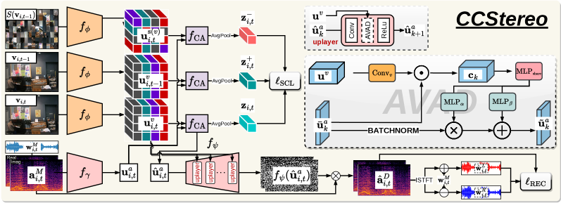
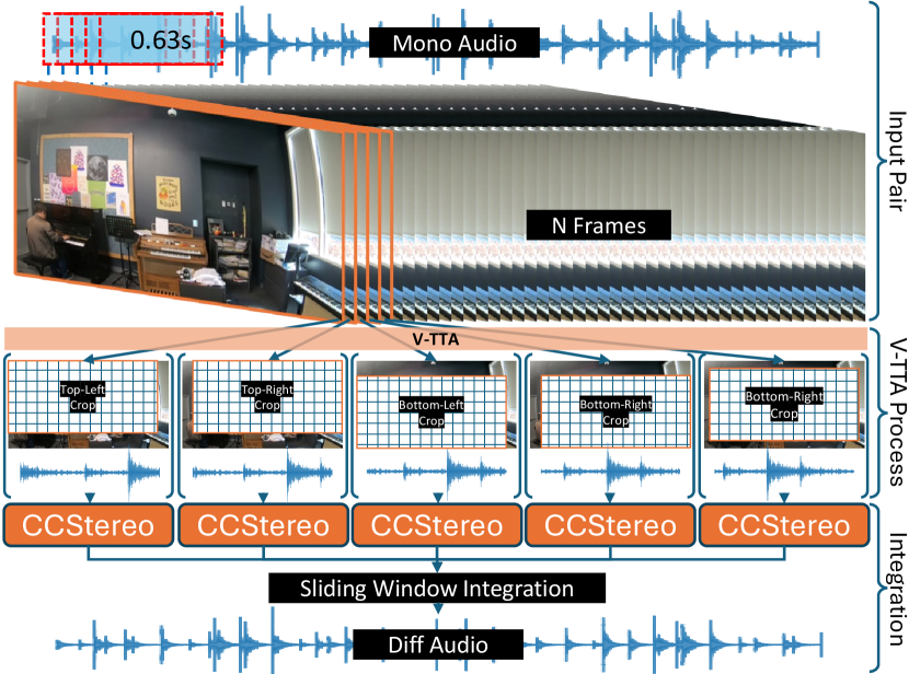
In this paper, we introduce a new U-Net-based generation framework that aims to mitigate the problems above, called Contextual and Contrastive Stereophonic Learning (CCStereo), which consists of a visually adaptive stereophonic learning method and a cost-effective inference strategy to enhance cross-modal interaction and mitigate overfitting by improving spatial reasoning. Unlike previous methods that rely solely on concatenated [4, 5, 6, 8, 13] or cross-attended [10] features for differential audio generation, we adopted the concept of conditional normalisation layers [14, 15, 12] from image synthesis field to control the generation process through estimated mean and variance shifts informed by visual context. Additionally, we propose a novel audio-visual contrastive learning method that enhances the model’s spatial sensitivity by incorporating contrastive learning across the feature maps of the anchor frame, nearby frames, and the spatially shuffled anchor frame. Moreover, the widely used sliding window inference strategy [4] introduces significant redundancy due to substantial frame overlap, which is common in video data. We argue that this overlap presents an opportunity to adopt test-time augmentation (TTA), leveraging the redundant information to enhance robustness and improve prediction accuracy. We introduce video test-time augmentation (V-TTA), which divides the video into sets of five consecutive frames and applies five-crop augmentation to each set across the entire video. To summarise, our main contributions are
-
•
A new audio-visual conditional normalisation layer that leverages visual context to dynamically align the mean and variance of the target difference audio features.
-
•
A novel audio-visual contrastive learning method that enhances spatial sensitivity by mining negative samples from randomly shuffled visual feature representations.
-
•
A cost-efficient approach for applying TTA to video data, improving robustness and prediction accuracy.
We demonstrate the effectiveness of our CCStereo model on established benchmarks, including the FAIR-Play dataset [4] with both the original 10-splits [4] and the more challenging 5-splits protocol [6]. Additionally, we extend our evaluation to the MUSIC-Stereo dataset [6], demonstrating generalisation across diverse audio-visual scenarios and superior generation quality with an efficient architecture. Code will be released.
II Related Works
Binaural audio generation (BAG) methods aim to create binaural audio from monaural recordings using visual information. Mono2Binaural [4], the first binaural audio generation method, uses a U-Net [16] to estimate the differential audio between the left and right channels by leveraging visual-spatial cues. However, operations like tiling and concatenation at the bottleneck layer [5] and average pooling [17] can lead to overfitting and loss of spatial details, limiting the model’s ability to capture complex spatial relationships. Enhancing the use of visual information in binaural audio generation has been a primary focus of recent research. Various methods are proposed to improve the model’s understanding of semantic and spatial information. These methods can broadly be categorised into three major directions: 1) improving cross-modal feature interaction [10] via attention mechanism [18] to better fuse the information between audio and visual modalities; 2) employing proxy learning tasks that help the model better understand the spatial correlation between the two modalities, such as discriminating the position of sound sources [13] or identifying their locations [9]; and 3) introducing the geometry clue of the scene, such as depth information [7] and room impulse response [11] to leverage the 3D environment during model reasoning. Additionally, prior studies [5, 6] have pointed out challenges like limited data availability and overfitting to visual environments. Efforts have been made to tackle these issues by using external monaural datasets [5] and reorganising benchmarks [6] to enhance model robustness and generalisation evaluation.
Conditional normalisation layers have been studied in style transfer [15] and conditional image synthesis [12]. Unlike standard normalisation methods [15] that rely on batch or instance statistics (e.g., mean and variance), conditional normalisation modulates these statistics through an affine transformation learned from external conditioning data [19]. In semantic image synthesis (e.g., SPADE [12]), this modulation is achieved using semantic segmentation maps, enabling the preservation of semantic information during decoding. Inspired by the SPADE layer, we incorporate spatially adaptive normalisation into the audio generation process, conditioning it on visual context to enable more precise control over the generation process.
Contrastive learning has shown promise in audio-visual learning methods [20, 21], aligning augmented representations of the same instance as positives while separating those of different instances as negatives within a batch. Binaural audio generation can similarly benefit from self-supervised learning tasks by leveraging contrastive objectives to distinguish left and right information in both audio [22] and visual [13] modalities.
Test-time augmentation (TTA) improves model performance by applying data augmentation at inference, creating multiple variations of the input and aggregating predictions. TTA is widely used in computer vision to enhance robustness without additional training [23]. Studies have shown that TTA effectively improves model generalisation [24], though it comes at the cost of significantly reduced inference speed. To handle moving sound sources and camera motion, previous binaural audio generation methods [4, 5, 6, 22, 9, 13] often adopted a sliding window strategy with a small hop size (e.g., 0.1), which leads to a large number of duplicated frames. We leverage this unique inference characteristic to integrate TTA into the process without incurring additional computational costs, thereby enhancing model performance.
III Method
We denote an unlabelled video dataset as , where is a set of RGB images with resolution , denotes the waveform data with channels and total number of sample . Given monaural audio (, We apply the short-time Fourier transform (STFT) [25] on , resulting in , where is the number of frequency bins and denotes the number of time frames. The model predicts the spectrogram of the target difference audio, defined as ().
Preliminaries. During training, we randomly sample an audio segment and its corresponding frame start at time step from each video (i.e., ) to form an input pair for the model. Our goal is to learn the parameters for the model , which comprises the image and audio encoder that extract features with and , respectively, where , and , with denoting a unified feature space. Our approach adopted a multi-head attention block [18], which estimates the co-occurrence of audio and visual data. We simply define the cross-attention process as , where represent the query and is the key and value. We decode the through an audio decoder , where . We use the MSE loss and magnitude loss [26] to constrain the prediction of the difference audio, where and is the modulus of the complex number. Different from [7], we argue that even though the phase of the difference audio is inherently linked to the phases of the left and right channels, it does not fully represent the binaural phase dynamics, hence apply the phase loss [7] on the final predicted binaural audio () and the ground truth binaural audio () instead of different audio. We denote the overall reconstruction loss as .
Audio-Visual Adaptive De-normalisation (AVAD). Our AVAD adopted the concept of conditional normalisation [14, 12] that leverages the interaction between audio and visual modality to control the normalisation of decoded feature representation. The AVAD is incorporated into the U-Net decoder by replacing the batch normalisation layers with visually-informed normalisation layers. This modification aims to effectively integrate both spatial and semantic information into the network’s input. Please note that, for simplicity, we omit the subscripts and in the following. As depicted in Fig. 1, we first pass through a batch normalisation layer (BN) at -th layer, and then scale and shift the normalised feature using the estimated and via . To compute these scaling factors, we calculate the similarity activate map and then estimate the scale () and shift () tensors through shared and specific MLP layers, such that and .
Spatial-aware Contrastive Learning (SCL). The capability to learn discriminative feature presentation is crucial for the audio-visual system. One limitation of previous binaural audio generation methods is their exclusive focus on proxy tasks within the audio domain (e.g., classifying whether the audio channels are flipped), which not only under-utilises visual positional information but also hinders the learning of a joint audio-visual representation. We argue that two requirements must be satisfied to achieve effective contrastive learning: 1) spatial awareness in the learned joint representation, and 2) inclusion of a diverse set of examples. Unfortunately, previous audio-visual contrastive learning methods [20, 21] may not be suitable for the current task, as they generally failed to satisfy these two requirements. Motivated by the Jigsaw puzzle self-supervised learning method [27], we observe that these two challenges can be addressed simultaneously by introducing perturbations to the visual-spatial order.
Since the BAG problem cannot access video-level labels, we adopt a classic instance discrimination pipeline (e.g., SimCLR [28]), where each audio-visual pair is treated as its own class. For a randomly sampled minibatch of examples, we perform the contrastive prediction task on pairs of positive and negative pairs derived from the minibatch. We define the anchor set , positive set and negative set as follows:
|
|
(1) |
where is the 2D average pooling and represent a shuffle process over the spatial dimension and of . Adopting the InfoNCE [28], we define the objective function as follows:
|
|
(2) |
where is an anchor feature, is its corresponding positive pair, are the negative features, and is the temperature hyperparameter.
Overall Training. The overall training objective is , where is a hyperparameter.
Video Test-Time Augmentation (V-TTA). During inference, we firstly estimate the left and right complex spectrograms through and . Then, we use inverse STFT (ISTFT) [25] to recover the audio signal from both channels and concatenate them together to form the final binaural waveform prediction . We use a sliding window of 0.63 seconds and a hop size of 0.1 seconds to binauralise 10-second audio clips, following an approach similar to that of the baseline methods [4]. While this process improves binaural audio generation by focusing on smaller audio segments, it introduces significant computational redundancy. Motivated by the small visual differences in 10 fps music videos, we design V-TTA to leverage this redundancy for better performance and robustness. As depicted in Fig. 2, instead of directly resizing every video frame to [4, 5, 6], we first resize each frame to and then crop a window from one of the five regions based on the current frame index (i.e., “ % 5”, where is a frame index). For example, if the first two audio segments are paired with the \nth5 and \nth6 frames, we crop the top-left corner of the \nth5 frame and the top-right corner of the \nth6 frame, respectively. Please refer to the Supplementary Material for additional details on sliding window integration.
| Methods | FAIR-Play (5-splits) [4, 6] | MUSIC-Stereo [29, 6] | ||||||||
|---|---|---|---|---|---|---|---|---|---|---|
| Mono-Mono [6] | 1.024 | 0.145 | 2.049 | 1.571 | 4.968 | 1.014 | 0.144 | 2.027 | 1.568 | 7.858 |
| Mono2Binaural [4, 6] | 0.917 | 0.137 | 1.835 | 1.504 | 5.203 | 0.942 | 0.138 | 1.885 | 1.550 | 8.255 |
| PseudoBinaural [6] | 0.944 | 0.139 | 1.901 | 1.522 | 5.124 | 0.943 | 0.139 | 1.886 | 1.562 | 8.198 |
| Sep-Stereo [5, 6] ★ | 0.906 | 0.136 | 1.811 | 1.495 | 5.221 | 0.929 | 0.135 | 1.803 | 1.544 | 8.306 |
| CMC [13] | - | - | - | - | - | 0.759 | 0.113 | 1.518 | 1.502 | - |
| BeyondM2B [7] | 0.909 | 0.139 | 1.819 | 1.479 | 6.397 | 0.670 | 0.108 | 1.340 | 1.538 | 10.754 |
| CCStereo | 0.883 | 0.137 | 1.766 | 1.454 | 6.475 | 0.624 | 0.097 | 1.248 | 1.578 | 12.985 |
| Methods | FAIR-Play (10-splits) [4, 6] | |||
|---|---|---|---|---|
| Mono2Binaural [4] | 0.959 | 0.141 | 6.496 | 6.232 |
| APNet [5] | 0.889 | 0.136 | 5.758 | 6.972 |
| Sep-stereo [5] ★ | 0.879 | 0.135 | 6.526 | 6.422 |
| Main Net. [10] | 0.867 | 0.135 | 5.750 | 6.985 |
| Complete Net. [10] | 0.856 | 0.134 | 5.787 | 6.959 |
| SAGM [8] | 0.851 | 0.134 | 5.684 | 7.044 |
| CMC [13] | 0.849 | 0.133 | - | - |
| CCStereo | 0.823 | 0.132 | 5.502 | 7.144 |
IV Experiments
IV-A Evaluation Protocols
Datasets. We adopt two widely used music video datasets FAIR-Play [4] and MUSIC-Stereo [29, 6] for the model evaluation process. The FAIR-Play [4] dataset contains 1,871 10-second clips of videos recorded in a music room, with a total playtime of 5.2 hours. The videos were recorded using a professional binaural microphone, preserving high-quality binaural audio. The FAIR-Play dataset has two commonly used train/validation/test split setups. The first is the 10-split setup [4], which randomly divides the videos into subsets. The second is the 5-split setup [6], designed to evaluate the model’s true generalisation ability by reducing scene overlap between training and testing, providing a more challenging evaluation setting. The videos are extracted to frames at 10 fps [4].
We also evaluate our approach on the MUSIC-Stereo dataset [6], which is based on the MUSIC dataset [29] containing 21 types of musical instruments, featuring both solo and duet performances. We follow previous works [5, 6, 7] by filtering out non-binaural cases using a threshold of 0.001 for the sum of left-right channel differences. We obtained 1,047 unique videos to have binaural audio. We then divided the videos into 80-10-10 for training, validation, and testing. Following previous works [6, 7], we split the videos into 10-second clips and finally arrived at 20,351 clips, which is 10x larger than the FAIR-Play dataset. As MUSIC-Stereo is a YouTube-based dataset, the total number of available samples may fluctuate. The videos are extracted to frames at 10 fps [6].
Evaluation Metrics. We follow the previous methods [5, 8, 6, 7] to report the STFT L2 distance (STFT), Magnitude distance (Mag) and Difference Phase Distance (Phs) on the time-frequency domain; and waveform L2 distance (WAV), envelope distance (ENV) and Signal-to-Noise Ratio (SNR) on time domain to assess the fidelity and quality of generated binaural audios.
| Method | Metrics | ||||||||
|---|---|---|---|---|---|---|---|---|---|
| Baseline | V-TTA | AVAD | |||||||
| ✔ | 0.941 | 0.145 | 1.881 | 1.525 | 6.043 | ||||
| ✔ | ✔ | 0.917 | 0.142 | 1.834 | 1.493 | 6.179 | |||
| ✔ | ✔ | ✔ | 0.908 | 0.140 | 1.815 | 1.486 | 6.254 | ||
| ✔ | ✔ | ✔ | ✔ | 0.891 | 0.139 | 1.783 | 1.453 | 6.371 | |
| ✔ | ✔ | ✔ | ✔ | ✔ | 0.885 | 0.138 | 1.771 | 1.451 | 6.457 |
IV-B Implementation Details
We follow previous methods [5, 8, 6, 7] to fix the audio sampling rate to 16 kHz and normalise each segment’s RMS level to a constant value. We adopted a widely used audio pre-processing protocol by applying the STFT with a Hann window of 25 ms, a hop length of 10 ms, and an FFT size of 512. During training, we randomly sample 0.63-second audio segments from each 10-second clip, along with the corresponding central visual frame. The selected frame is resized to 480×240, then randomly cropped to 448×224. We also apply colour and intensity jittering as data augmentation, following [4]. We use a convolutional U-Net architecture [4] for the audio backbone and a ResNet [30] (pre-trained on ImageNet [31]) for the image backbone. The networks are trained using the Adam optimiser with a learning rate of 5e-5 for the image backbone and 5e-4 for the audio backbone, using a batch size of 128. We set to 0.1.
IV-C Results
Results on FAIR-Play Dataset. We adopt established benchmarks for conducting model evaluations, such as FAIR-Play 10-splits [4] and 5-splits [6]. We first show the comparison on FAIR-Play 10-splits [4] benchmark in Tab. II. The results demonstrate that our model surpasses the second-best models by in STFT, in ENV, in WAV, and in SNR, respectively. Please note that we exclude CLUP [9] from this table, as it introduces additional computational complexity (e.g., diffusion [32] and VGGish [33]) and their method is not publicly available for inference comparison. To evaluate the true generalisation ability as suggested by PseudoBinaural [6], we also utilise the newly proposed FAIR-Play (5-split) [6] for the evaluation, as shown in the left part of Tab. I. Our method outperforms the second-best model by in STFT, in Mag, in Phs, and in SNR.
Results on MUSIC-STEREO Dataset. To further evaluate model scalability and generalisability on larger-scale datasets, we follow [6, 7] to assess performance on the MUSIC-STEREO dataset [6], as shown in the right part of Tab. I. Our method outperforms the second-best method by in STFT, in ENV, in Mag, and in SNR. The results indicate that our method achieves higher prediction fidelity and contains less noise relative to the signal, demonstrating that CCStereo generalises better in complex scenarios.
IV-D Ablation Study
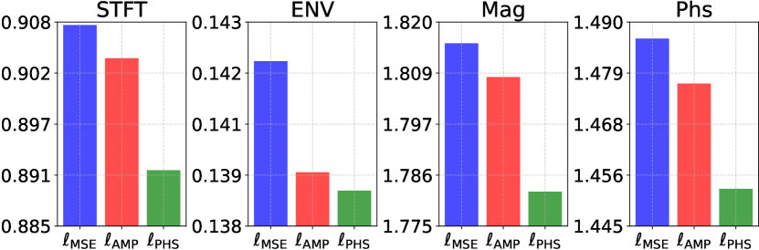
We perform an analysis of CCStereo components on the second split of FAIR-Play (5-split)[6], as shown in Tab.III. Starting from a baseline (1st row) consisting of a simple U-Net model similar to Mono2Binaural [4] that resizes the input frame directly to 448224 during the inference. We utilise the V-TTA method to enhance the inference process, resulting in a STFT improvement of . Integrating AVAD into the system (3rd row) provides an additional improvement of . Subsequently, adding and (i.e., ) (4th row) and incorporating the contrastive learning method (5th row) yield further improvements of and , respectively. To separately analyse each loss term in , we conducted an ablation study, as shown in Fig.4, to evaluate the individual contributions of and . Starting with the third row in Tab.III, we progressively added and during model training. We observed improvements of and on STFT, respectively, highlighting the importance of aligning phase information for accurate binaural prediction.
IV-E Qualitative Results
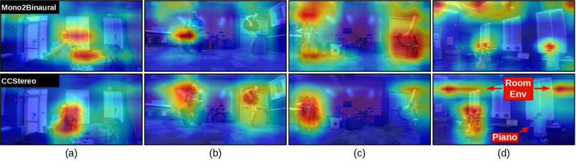
We present qualitative results of visual activation estimated by our method in Fig. 3. Specifically, we extract the output from the convolution layer for Mono2Binaural [4] and AVAD, average the activation map across channels, and normalise it using min-max normalisation. The results in Fig. 3a, 3b, 3c indicate that our method can better focus on the sounding object and its position. However, Tab. 3d illustrates a failure case, where the model is unable to localise the occluded object “piano” and instead shows a tendency to focus on the room environment (Room Env). We hypothesise that when the model fails to identify the sounding object, it associates the audio with the room environment. These observations highlight the limitations of the current method. For further results on videos, please refer to the Supplementary Material.
V Discussion and Conclusion
We introduced CCStereo, a new audio-visual training method designed for the U-Net-based framework to enhance spatial awareness and reduce overfitting to room environments. We proposed a visually conditioned adaptive de-normalisation method that utilises the object’s spatial information to guide the decoding of the difference audio. To enhance the representation learning of spatial awareness, we design a new audio-visual contrastive learning based on mining negative samples from randomly shuffled visual feature representation. Furthermore, our cost-efficient test-time augmentation strategy enhanced robustness without adding computational overhead. Our approach consistently outperformed existing methods on the FAIR-Play and MUSIC-Stereo datasets, achieving state-of-the-art results across various metrics.
References
- [1] Emil R Hoeg, Lynda J Gerry, Lui Thomsen, Niels C Nilsson, and Stefania Serafin, “Binaural sound reduces reaction time in a virtual reality search task,” in SIVE. IEEE, 2017, pp. 1–4.
- [2] Pedro Morgado, Nuno Nvasconcelos, Timothy Langlois, and Oliver Wang, “Self-supervised generation of spatial audio for 360 video,” NeurIPS, vol. 31, 2018.
- [3] David Griesinger, “Binaural techniques for music reproduction,” in Audio Engineering Society Conference: 8th International Conference: The Sound of Audio. Audio Engineering Society, 1990.
- [4] Ruohan Gao and Kristen Grauman, “2.5 d visual sound,” in CVPR, 2019, pp. 324–333.
- [5] Hang Zhou, Xudong Xu, Dahua Lin, Xiaogang Wang, and Ziwei Liu, “Sep-stereo: Visually guided stereophonic audio generation by associating source separation,” in ECCV. Springer, 2020, pp. 52–69.
- [6] Xudong Xu, Hang Zhou, Ziwei Liu, Bo Dai, Xiaogang Wang, and Dahua Lin, “Visually informed binaural audio generation without binaural audios,” in CVPR, 2021, pp. 15485–15494.
- [7] Kranti Kumar Parida, Siddharth Srivastava, and Gaurav Sharma, “Beyond mono to binaural: Generating binaural audio from mono audio with depth and cross modal attention,” in Proceedings of the IEEE/CVF Winter Conference on Applications of Computer Vision, 2022, pp. 3347–3356.
- [8] Zhaojian Li, Bin Zhao, and Yuan Yuan, “Cross-modal generative model for visual-guided binaural stereo generation,” Knowledge-Based Systems, vol. 296, pp. 111814, 2024.
- [9] Zhaojian Li, Bin Zhao, and Yuan Yuan, “Cyclic learning for binaural audio generation and localization,” in CVPR, 2024, pp. 26669–26678.
- [10] Wen Zhang and Jie Shao, “Multi-attention audio-visual fusion network for audio spatialization,” in ICMR, 2021, pp. 394–401.
- [11] Rishabh Garg, Ruohan Gao, and Kristen Grauman, “Geometry-aware multi-task learning for binaural audio generation from video,” BMVC, 2021.
- [12] Taesung Park, Ming-Yu Liu, Ting-Chun Wang, and Jun-Yan Zhu, “Semantic image synthesis with spatially-adaptive normalization,” in CVPR, 2019, pp. 2337–2346.
- [13] Miao Liu, Jing Wang, Xinyuan Qian, and Xiang Xie, “Visually guided binaural audio generation with cross-modal consistency,” in ICASSP 2024-2024 IEEE International Conference on Acoustics, Speech and Signal Processing (ICASSP). IEEE, 2024, pp. 7980–7984.
- [14] Xun Huang and Serge Belongie, “Arbitrary style transfer in real-time with adaptive instance normalization,” in Proceedings of the IEEE international conference on computer vision, 2017, pp. 1501–1510.
- [15] Hyeonseob Nam and Hyo-Eun Kim, “Batch-instance normalization for adaptively style-invariant neural networks,” NeurIPS, vol. 31, 2018.
- [16] Olaf Ronneberger, Philipp Fischer, and Thomas Brox, “U-net: Convolutional networks for biomedical image segmentation,” in MICCAI. Springer, 2015, pp. 234–241.
- [17] Hossein Gholamalinezhad and Hossein Khosravi, “Pooling methods in deep neural networks, a review,” arXiv preprint arXiv:2009.07485, 2020.
- [18] A Vaswani, “Attention is all you need,” NeurIPS, 2017.
- [19] Rameen Abdal, Peihao Zhu, Niloy J Mitra, and Peter Wonka, “Styleflow: Attribute-conditioned exploration of stylegan-generated images using conditional continuous normalizing flows,” ACM ToG, vol. 40, no. 3, pp. 1–21, 2021.
- [20] Honglie Chen, Weidi Xie, Triantafyllos Afouras, Arsha Nagrani, Andrea Vedaldi, and Andrew Zisserman, “Localizing visual sounds the hard way,” in CVPR, 2021, pp. 16867–16876.
- [21] Yuanhong Chen, Yuyuan Liu, Hu Wang, Fengbei Liu, Chong Wang, Helen Frazer, and Gustavo Carneiro, “Unraveling instance associations: A closer look for audio-visual segmentation,” in CVPR, 2024, pp. 26497–26507.
- [22] Sijia Li, Shiguang Liu, and Dinesh Manocha, “Binaural audio generation via multi-task learning,” ACM TOG, vol. 40, no. 6, pp. 1–13, 2021.
- [23] Masanari Kimura, “Understanding test-time augmentation,” in International Conference on Neural Information Processing. Springer, 2021, pp. 558–569.
- [24] Jason Wang, Luis Perez, et al., “The effectiveness of data augmentation in image classification using deep learning,” Convolutional Neural Networks Vis. Recognit, vol. 11, no. 2017, pp. 1–8, 2017.
- [25] Daniel Griffin and Jae Lim, “Signal estimation from modified short-time fourier transform,” IEEE Transactions on acoustics, speech, and signal processing, vol. 32, no. 2, pp. 236–243, 1984.
- [26] Alexander Richard, Dejan Markovic, Israel D Gebru, Steven Krenn, Gladstone Alexander Butler, Fernando Torre, and Yaser Sheikh, “Neural synthesis of binaural speech from mono audio,” in ICLR, 2021.
- [27] Mehdi Noroozi and Paolo Favaro, “Unsupervised learning of visual representations by solving jigsaw puzzles,” in ECCV. Springer, 2016, pp. 69–84.
- [28] Ting Chen, Simon Kornblith, Mohammad Norouzi, and Geoffrey Hinton, “A simple framework for contrastive learning of visual representations,” in International conference on machine learning. PMLR, 2020, pp. 1597–1607.
- [29] Hang Zhao, Chuang Gan, Andrew Rouditchenko, Carl Vondrick, Josh McDermott, and Antonio Torralba, “The sound of pixels,” in ECCV, 2018, pp. 570–586.
- [30] Kaiming He, Xiangyu Zhang, Shaoqing Ren, and Jian Sun, “Deep residual learning for image recognition,” in CVPR, 2016, pp. 770–778.
- [31] Jia Deng, Wei Dong, Richard Socher, Li-Jia Li, Kai Li, and Li Fei-Fei, “Imagenet: A large-scale hierarchical image database,” in CVPR. Ieee, 2009, pp. 248–255.
- [32] Jonathan Ho, Ajay Jain, and Pieter Abbeel, “Denoising diffusion probabilistic models,” NeurIPS, vol. 33, pp. 6840–6851, 2020.
- [33] Shawn Hershey, Sourish Chaudhuri, Daniel PW Ellis, Jort F Gemmeke, Aren Jansen, R Channing Moore, Manoj Plakal, Devin Platt, Rif A Saurous, Bryan Seybold, et al., “Cnn architectures for large-scale audio classification,” in ICASSP. IEEE, 2017, pp. 131–135.