Cell-Free Symbiotic Radio: Channel Estimation Method and Achievable Rate Analysis
Abstract
Cell-free massive MIMO and symbiotic radio are promising beyond 5G (B5G) networking architecture and transmission technology, respectively. This paper studies cell-free symbiotic radio systems, where a number of distributed access points (APs) cooperatively send primary information to a receiver, and simultaneously support the backscattering communication of the secondary backscatter device (BD). An efficient two-phase uplink-training based channel estimation method is proposed to estimate the direct-link channel and cascaded backscatter channel, and the achievable primary and secondary communication rates taking into account the channel estimation errors are derived. Furthermore, to achieve a flexible trade-off between the primary and secondary communication rates, we propose a low-complexity weighted-maximal-ratio transmission (weighted-MRT) beamforming scheme, which only requires local processing at each AP without having to exchange the estimated channel state information. Simulation results are provided to show the impact of the channel training lengths on the performance of the cell-free symbiotic radio systems.
I Introduction
Along with the rapid deployment of the fifth-generation (5G) mobile communication networks, researchers have started the investigation of 6G targeting for network 2030 [1, 2]. In order to support orders-of-magnitude performance improvement in terms of coverage, connectivity density, data rate, reliability, latency, etc., many promising technologies have been extensively studied, such as extremely large-scale MIMO/surface [3, 4], TeraHertz communication [5], non-terrestrial networks (NTN) [6, 7], and AI-aided wireless communications [8]. In particular, cell-free massive MIMO [9] and symbiotic radio [10] were recently proposed as promising networking architecture and transmission technology for beyond 5G (B5G), respectively.
Cell-free massive MIMO is different from the classical cellular networking architecture in the sense that it blurs the conventional concepts of cells or cell boundary [9]. Instead, distributed access points (APs), which are connected to the central processing unit (CPU), exploit their local channel state information (CSI) to simultaneously serve the users. As such, cell-free massive MIMO system is expected to mitigate the inter-cell interference issues in small cell systems and provides users with appealing uniform good service everywhere [11]. Meanwhile, no exchange of CSI is required among different APs, which enables low complexity and light backhaul load between APs and CPU. Therefore, significant research efforts have been recently devoted to the theoretical analysis and practical design of cell-free massive MIMO, e.g., precoding design [12], power optimization [9], and energy efficiency analysis [13, 14].
On the other hand, in terms of transmission technology for B5G, symbiotic radio, which combines the benefits of the conventional cognitive radio (CR) and ambient backscattering communications (AmBC), has been proposed for spectral- and energy-efficient communications [10]. In typical symbiotic radio systems, the secondary device not only utilizes the spectral but also the power of the primary system via the passive backscattering technology [15]. Based on the relationship of symbol durations of the primary and the secondary signals, symbiotic radio system can be classified as commensal symbiotic radio (CSR) and parasite symbiotic radio (PSR) [16]. In CSR, the secondary signals have much longer symbol duration than the primary signals, making the secondary backscattering transmission contribute additional multipath components to enhance the primary communication. As a result, the primary and secondary communications form a mutualism relationship [16]. By contrast, in PSR, the primary and secondary signals have equal symbol duration, and the secondary signals are often treated as interference to the primary signals. Significant research efforts have been recently devoted to the study of symbiotic radio systems, e.g., in terms of performance analysis [17] and resource allocations [18, 19].
However, all the aforementioned existing works studied cell-free massive MIMO and symbiotic radio separately, i.e., cell-free system with the conventional active transmission or symbiotic radio transmission in conventional cellular network or the basic point-to-point communications. As the promising B5G networking architecture and transmission technology, respectively, it is natural that cell-free networking and symbiotic radio communication would merge each other to reap the benefits of both. This thus motivates our current work to study cell-free symbiotic radio systems, which, to our best knowledge, have not been studied in the existing literature. In cell-free symbiotic radio systems, a number of distributed APs cooperatively send primary information to a receiver, and concurrently support the passive backscattering communication of the secondary backscatter device (BD). As such, the distributed cooperation gain by APs can be exploited to enhance both the primary and secondary communication rate. An efficient two-phase uplink-training based channel estimation method is proposed to estimate the direct-link channel and cascaded backscatter channel, respectively. Furthermore, the interrelationship between the primary and secondary transmission is revealed by deriving their achievable rates taking into account the channel estimation errors. Besides, to achieve a flexible trade-off between the primary and secondary communication rate, a low-complexity weighted-maximal-ratio transmission (weighted-MRT) beamforming scheme is proposed, which only requires local processing at each AP without having to exchange the estimated CSI among APs. Numerical results are provided to show the performance of the cell-free symbiotic radio system with different training lengths.
II System Model
As shown in Fig. 1, we consider a cell-free symbiotic radio system, which consists of distributed APs, one information receiver, and one BD. The APs cooperatively send primary information to the receiver, and simultaneously support the BD for secondary communication via backscattering to the same receiver. The considered setup may model a wide range of applications, e.g., with the receiver corresponding to smartphones and the BD being the smart home sensor nodes.
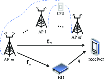
We assume that each AP is equipped with antennas, and the receiver and BD each has one antenna. Denote by and the multiple-input single-output (MISO) channels from the th AP to the receiver and BD, respectively, where . Further denote by the channel coefficient from the BD to the receiver. Then, the cascaded backscatter channel from the th AP to the receiver via the BD is .
In this paper, we focus on the PSR setup[16], where the symbol duration of the primary and secondary signals are equal. Let and denote the circularly symmetric complex Gaussian (CSCG) information-bearing symbols of the primary and secondary signals respectively. Further denote by the transmit power of each AP, and with denotes the transmit beamforming vector of the th AP. Then the received signal at the receiver is
| (1) |
where denotes the power reflection coefficient, is the additive white Gaussian noise. Based on the received signal in (1), the receiver wishes to decode both the primary and secondary signals. To that end, since the backscatter link is typically much weaker than the direct link, the receiver may first decode the primary symbols , by treating the backscattered signals as noise, whose power is . Therefore the signal-to-interference-plus-noise ratio (SINR) for decoding the primary information is
| (2) |
Note that due to the product of and in the second term of (1), the resulting noise for decoding is no longer Gaussian. However, by using the fact that for any given noise power, Gaussian noise results in the maximum entropy and hence constitutes the worst-case noise [21, 20], the achievable rate of the primary signal in (1) is
| (3) |
After decoding the primary information, the first term in (1) can be subtracted from the received signal before decoding the secondary symbols . The resulting signal is
| (4) |
Note that since varies across different secondary symbols , (4) can be interpreted as a fast-fading channel, whose instantaneous channel gain depends on [22]. With , its squared envelope follows an exponential distribution. Therefore, the ergodic rate of the backscatter communication (4) can be expressed as [16, 23]
| (5) | ||||
where is the exponential integral, and is the average received SNR of the backscatter link.
Note that the above analysis is based on the assumption of perfect CSI on , , and . In practical wireless communication systems, these channels need to be acquired via e.g., pilot-based channel estimation. In the following, we propose the channel estimation methods for cell-free symbiotic radio systems and analyze the achievable rates taking into account the channel estimation errors.
III Channel Estimation and Achievable Rate Analysis
Similar to the extensively studied massive MIMO systems, efficient channel estimation for cell-free massive MIMO can be achieved by exploiting the uplink-downlink channel reciprocity [24, 25], i.e., the downlink channels can be efficiently estimated via uplink training. However, different from the existing cell-free massive MIMO systems [9], the channel estimation for cell-free symbiotic radio requires estimating not only the direct-link channels , but also the backscatter channels and . To this end, in the following, we propose a two-phase based channel estimation method for cell-free symbiotic radio systems. In the first phase, pilot symbols are sent by the receiver while muting the BD, so as to estimate the direct-link channels . In the second phase, pilots are sent both by the receiver and the BD so that, together with the estimation of the direct-link channels, the cascaded backscatter channels , are estimated.
III-A Direct-Link Channel Estimation
First, we discuss the uplink training-based estimation of the direct-link channels between the receiver and the APs. Denote by the length of the uplink training sequence, and let be the training power. Further denote by the pilot sequence, where . The received training signals by the antennas of the th AP over the symbol durations, which is denoted as , can be written as
| (6) |
where denotes the i.i.d CSCG noise with zero-mean and power . With the pilot sequence known at the APs, can be projected to , which gives
| (7) |
where is the resulting noise vector. It can be shown that is i.i.d. CSCG noise with power , i.e., .
With being a zero-mean random vector, its linear minimum mean square error estimation (LMMSE), denoted by , is [26]
| (8) | ||||
where denotes the covariance matrix of . By further decomposing the direct-link channel as , with denoting the large-scale channel coefficient, and denoting the zero-mean CSCG small-scale fading component, i.e., . Then is CSCG distributed with covariance matrix , and thus LMMSE estimation is also the optimal MMSE estimation. In this case, (8) can be simplified as
| (9) |
It can be shown that follows the distribution
| (10) |
where we have defined the transmit training energy-to-noise ratio (ENR) as .
Let denote the channel estimation error of the th AP, i.e., . With MMSE estimation, it is known that is uncorrelated with [26], which follows the distribution
| (11) |
It is observed from (11) that as the transmit training ENR increases, the variance of the channel estimation error reduces, as expected.
III-B Backscatter Channel Estimation
With the estimation for the direct-link channels, in the second phase, pilot symbols are sent from both the receiver and the BD to estimate the cascaded backscatter channels , . Let denote the length of the training sequence in the second phase and be the pilot sequence sent by the receiver, with . The received training signal by the th AP can be written as
| (12) |
where denotes the i.i.d. CSCG noise with power . Note that without loss of generality, we assume that the pilot symbols backscattered by the BD are all . After subtracting the terms related to the estimation of the direct-link channels from (12), we have
| (13) |
With known at the APs, the projection of after scaling by , is
| (14) |
where we have defined the cascaded backscatter channel as , and . It can be shown that .
Let denote the covariance matrix of the cascaded backscatter channel . Then the LMMSE estimation of based on (14) is
| (15) | ||||
where is the covariance matrix of .
If the channel coefficients in are i.i.d. distributed with variance , we then have , where and .
As a result, (15) can be simplified as
| (16) |
Define the transmit training ENR in the second phase as . It then follows from (11) and (16) that
| (17) |
Let denote the estimation error. We have
| (18) | ||||
It follows from (11) that if , in which case the direct-link channel is perfectly estimated without any error, the variance of the estimation error in (18) reduces to the same form as that in (11).
III-C Achievable Rate Analysis
In this subsection, we derive the achievable primary and secondary rates based on the channel estimation and , by taking into account the channel estimation errors. By substituting and into (1), the received signal for information transmission can be written as
| (19) | ||||
For decoding the primary signals , besides the interference from the backscatter symbols , the term caused by the channel estimation error is also treated as noise [27, 21]. Therefore, (19) can be decomposed as
| (20) |
where , and denote the desired signal, estimation errors and the secondary transmission signal respectively, which are given by
| (21) |
| (22) |
| (23) |
Therefore, the resulting SINR can be expressed as (24) shown at the top of the next page, and the achievable rate is .
| (24) | ||||
Note that for any given channel estimations and , since the channel estimation errors and are random, the SINR in (24) and hence its rate is random. By taking the expected achievable rate with respect to the random estimation errors and , we have the result (25) shown at the top of the next page, where accounts for the average channel estimation error and noise. Note that the inequality in (25) follows from Jensen’s inequality, and the fact that is a convex function for .
| (25) | ||||
Next, we derive the achievable rate of the secondary signals . After decoding , the primary signals can be subtracted from (19) based on the estimated channel . The resulting signal is
| (26) | ||||
By treating the terms caused by the channel estimation error and as noise, (26) can be decomposed as
| (27) |
where denotes the estimation errors given in (22), and denotes the desired signal, which is given by
| (28) |
The resulting SINR is
| (29) | ||||
and the achievable rate is .
Note that different from (24), as the desired channel also depends on the primary symbols , the SNR in (29) is a random variable that depends on both and the channel estimation errors. Consider the expectation of , with the expectation taken with respect to both and the channel estimation errors, we have
| (30) | ||||
where the inequality is obtained by applying Jensen’s inequality to the convex function , and represents the average SNR for the secondary signals taking into account the channel estimation errors.
III-D Weighted-MRT Beamforming
It can be observed from (25) and (30) that for cell-free symbiotic systems, the achievable primary and secondary communication rates depend on the transmit beamforming vectors . In particular, in order to maximize the primary communication link, all the APs set their beamforming vector as the MRT beamforming vector matched to the estimated direct-link channel , which is
| (31) |
On the other hand, to maximize the secondary communication rate in (30), is set as the MRT beamformer matched to the estimated backscatter link , which is
| (32) |
In order to achieve a flexible trade-off between the primary and secondary communication rate, in this paper, we propose a low-complexity weighted-MRT beamforming scheme, where the transmit beamforming vector for each AP is set as
| (33) |
where is a weighting coefficient that controls the trade-off between the primary and secondary communication rate, and is a power normalization factor to ensure for any given . By varying between 0 and 1, the achievable rate regions of the primary and secondary transmission can be obtained. Note that weighted-MRT beamforming is especially appealing for cell-free symbiotic radio systems, due to its low-complexity and scalability, since each AP can perform the beamforming locally with its own channel estimations and , without having to exchange the estimated CSIs among APs.
IV Simulation Results
In this section, simulation results are provided to evaluate the performance of cell-free symbiotic radio systems. We set up a Cartesian coordinate system, where the BD is located at the origin (0,0), and the receiver is located at (5m, 0). Furthermore, we assume that APs, each with antennas, are evenly spaced in a square area of size , i.e., their locations correspond to the grid points, with the x- and y-coordinates chosen from the set {-375m, -125m, 125m, 375m}. The channels of all communication links are independent, where the small-scale fading coefficients follow the i.i.d. CSCG distribution with zero mean and unit variance. Furthermore, the large-scale channel gains of all links are modeled as , where is the reference channel gain with m denoting the wavelength, represents the corresponding link distance, and denotes the path loss exponent. We set for the AP-to-BD and AP-to-receiver channels, and for BD-to-receiver channels. The power reflection coefficient is , and the transmitter-side SNR for both information and pilot transmission is set as dB, which may correspond to dBm and dBm. The simulation results are obtained by taking the average values over 1000 channel realizations.
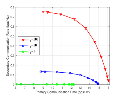
Fig. 2 shows the achievable rate regions of the primary and secondary rates with different uplink training lengths , and hence different training ENR , while the pilot length in the second training phase is fixed to . Note that each point of the curve corresponds to a primary-secondary rate pair with the weighted-MRT beamforming (33), by varying the weight from 0 to 1 with step size 0.1. It is observed from Fig. 2 that with the training SNR and training length fixed, the achievable rate regions critically depend on the training length . For , which corresponds to low training ENR in the first phase, the secondary communication rate is almost zero, regardless of the beamforming weight . This can be explained by the fact that when is low, there exists severe channel estimation error for the direct-link channel estimation, whose detrimental effect will be exacerbated for the estimation of the weaker cascaded backscatter channels in the second training phase. This thus severely limits the achievable rate of the secondary backscattering communication. As increases to 100 so that both the direct-link and backscatter channels are estimated more accurately, the rate region enlarges significantly.
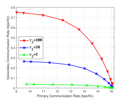
By fixing , Fig. 3 plots the achievable rate regions with different training lengths in the second phase. Similar to Fig. 2, it is observed from Fig. 3 that the rate region enlarges significantly as increases, as expected. It is also interesting to note that with larger , the minimum primary communication rate (corresponding to ) actually reduces. This can be explained by the fact that as the cascaded backscatter channels are estimated more accurately with larger , it results in stronger interference to the primary communication with MRT beamforming matched to the secondary link, which thus decreases the minimum primary rate. However, the maximum primary rate () is almost unaffected by . By comparing Fig. 2 and Fig. 3, it is also observed that larger rate regions are achieved for and in Fig. 3 than its counterpart in Fig. 2. This implies that if the total training length is fixed, higher priority should be given to the first training phase. This is expected since the estimation of the direct-link channels in the first phase impacts not only the primary communication rate, but also the quality of the channel estimation of the backscatter channels.
V Conclusion
In this paper, a novel cell-free symbiotic radio system was studied, in which a number of distributed APs cooperatively send primary information, while concurrently supporting the secondary backscattering communication. A two-phase uplink-training based channel estimation method was proposed to estimate the direct-link channel and cascaded backscatter channel. Furthermore, a low-complexity weighted-MRT beamforming scheme was proposed to achieve a flexible trade-off between the primary and secondary communication rate. Simulation results were provided to demonstrate the performance of the cell-free symbiotic radio systems.
Acknowledgment
This work was supported by the National Key R&D Program of China with Grant number 2019YFB1803400.
References
- [1] M. Latva-aho and K. L. (eds.), “Key drivers and research challenges for 6G ubiquitous wireless intelligence,” 6G Research Visions 1, 6G Flagship, University of Oulu, Finland, Sep. 2019.
- [2] X. You et al., “Towards 6G wireless communication networks: vision, enabling technologies, and new paradigm shifts,” Sci. China Inf. Sci., vol. 64, no. 1, pp. 1–74, Nov. 2020.
- [3] S. Hu, F. Rusek, and O. Edfors, “Beyond massive MIMO: The potential of data transmission with large intelligent surfaces,” IEEE Trans. Signal Process. , vol. 66, no. 10, pp. 2746–2758, Mar. 2018.
- [4] H. Lu and Y. Zeng, “Communicating with extremely large-scale array/surface: unified modelling and performance analysis,” arXiv preprint arXiv:2104.13162, 2021.
- [5] H. Elayan, O. Amin, R. M. Shubair, and M.-S. Alouini, “Terahertz communication: The opportunities of wireless technology beyond 5G,” in Proc. IEEE Int. Conf. Adv. Commun. Technol. Netw.(CommNet), Apr. 2018, pp. 1–5.
- [6] M. Giordani and M. Zorzi, “Non-terrestrial networks in the 6G era: Challenges and opportunities,” IEEE Netw., vol. 35, no. 2, pp. 244–251, Dec. 2021.
- [7] Y. Zeng, Q. Wu, and R. Zhang, “Accessing from the sky: A tutorial on uav communications for 5G and beyond,” Proc. IEEE, vol. 107, no. 12, pp. 2327–2375, Dec. 2019.
- [8] N. C. Luong, D. T. Hoang, S. Gong, D. Niyato, P. Wang, Y.-C. Liang, and D. I. Kim, “Applications of deep reinforcement learning in communications and networking: A survey,” IEEE Commun. Surv. Tutor., vol. 21, no. 4, pp. 3133–3174, May. 2019.
- [9] H. Q. Ngo, A. Ashikhmin, H. Yang, E. G. Larsson, and T. L. Marzetta, “Cell-free massive MIMO versus small cells,” IEEE Trans. Wirel. Commun., vol. 16, no. 3, pp. 1834–1850, Jan. 2017.
- [10] Y.-C. Liang, Q. Zhang, E. G. Larsson, and G. Y. Li, “Symbiotic radio: Cognitive backscattering communications for future wireless networks,” IEEE Trans. Cogn. Commun. Netw., vol. 6, no. 4, pp. 1242–1255, Sep. 2020.
- [11] G. Interdonato, E. Björnson, H. Q. Ngo, P. Frenger, and E. G. Larsson, “Ubiquitous cell-free massive MIMO communications,” EURASIP J. Wireless Commun. Netw., pp. 1–19, Aug. 2019.
- [12] E. Nayebi, A. Ashikhmin, T. L. Marzetta, H. Yang, and B. D. Rao, “Precoding and power optimization in cell-free massive MIMO systems,” IEEE Trans. Wirel. Commun., vol. 16, no. 7, pp. 4445–4459, May. 2017.
- [13] L. D. Nguyen, T. Q. Duong, H. Q. Ngo, and K. Tourki, “Energy efficiency in cell-free massive MIMO with zero-forcing precoding design,” IEEE Commun. Lett., vol. 21, no. 8, pp. 1871–1874, Apr. 2017.
- [14] H. Q. Ngo, L.-N. Tran, T. Q. Duong, M. Matthaiou, and E. G. Larsson, “On the total energy efficiency of cell-free massive MIMO,” IEEE Trans. Green Commun. Netw., vol. 2, no. 1, pp. 25–39, Nov. 2018.
- [15] R. Long, H. Guo, L. Zhang, and Y.-C. Liang, “Full-duplex backscatter communications in symbiotic radio systems,” IEEE Access, vol. 7, pp. 21 597–21 608, Feb. 2019.
- [16] R. Long, Y.-C. Liang, H. Guo, G. Yang, and R. Zhang, “Symbiotic radio: A new communication paradigm for passive internet of things,” IEEE Internet Things J., vol. 7, no. 2, pp. 1350–1363, Nov 2020.
- [17] T. Wu, M. Jiang, Q. Zhang, Q. Li, and J. Qin, “Beamforming design in multiple-input-multiple-output symbiotic radio backscatter systems,” IEEE Commun. Lett., pp. 1–1, Feb. 2021.
- [18] H. Guo, Y.-C. Liang, R. Long, S. Xiao, and Q. Zhang, “Resource allocation for symbiotic radio system with fading channels,” IEEE Access, vol. 7, pp. 34 333–34 347, Mar. 2019.
- [19] Z. Chu, W. Hao, P. Xiao, M. Khalily, and R. Tafazolli, “Resource allocations for symbiotic radio with finite blocklength backscatter link,” IEEE Internet Things J., vol. 7, no. 9, pp. 8192–8207, Mar, 2020.
- [20] F. Neeser and J. Massey, “Proper complex random processes with applications to information theory,” IEEE Trans. Inf. Theory, vol. 39, no. 4, pp. 1293–1302, Jul. 1993.
- [21] B. Hassibi and B. Hochwald, “How much training is needed in multiple-antenna wireless links?” IEEE Trans. Inf. Theory, vol. 49, no. 4, pp. 951–963, Apr. 2003.
- [22] Q. Zhang, L. Zhang, Y.-C. Liang, and P.-Y. Kam, “Backscatter-noma: A symbiotic system of cellular and Internet-of-Things networks,” IEEE Access, vol. 7, pp. 20 000–20 013, Feb. 2019.
- [23] D. Tse and P. Viswanath, Fundamentals of Wireless Communication. Cambridge, U.K.: Cambridge Univ. Press, 2005.
- [24] F. Kaltenberger, H. Jiang, M. Guillaud, and R. Knopp, “Relative channel reciprocity calibration in MIMO/TDD systems,” in Proc. Future Network and Mobile Summit, Florence, Italy, Jun. 2010, pp. 1-10.
- [25] T. L. Marzetta, “Noncooperative cellular wireless with unlimited numbers of base station antennas,” IEEE Trans. Wirel. Commun., vol. 9, no. 11, pp. 3590–3600, Oct. 2010.
- [26] S. K. Sengijpta, “Fundamentals of statistical signal processing: Estimation theory,” Oxford, U.K.: Taylor & Francis, 1995.
- [27] Y. Zeng, R. Zhang, and Z. N. Chen, “Electromagnetic lens-focusing antenna enabled massive MIMO: Performance improvement and cost reduction,” IEEE J. Sel. Areas Commun., vol. 32, no. 6, pp. 1194–1206, Jun. 2014.