Chance-constrained OPF: A Distributed Method with Confidentiality Preservation
Abstract
Given the increased percentage of wind power in power systems, chance-constrained optimal power flow (CC-OPF) calculation, as a means to take wind power uncertainty into account with a guaranteed security level, is being promoted. Compared to the local CC-OPF within a regional grid, the global CC-OPF of a multi-regional interconnected grid is able to coordinate across different regions and therefore improve the economic efficiency when integrating high percentage of wind power generation. In this global problem, however, multiple regional independent system operators (ISOs) participate in the decision-making process, raising the need for distributed but coordinated approaches. Most notably, due to regulation restrictions, commercial interest, and data security, regional ISOs may refuse to share confidential information with others, including generation cost, load data, system topologies, and line parameters. But this information is needed to build and solve the global CC-OPF spanning multiple areas. To tackle these issues, this paper proposes a distributed CC-OPF method with confidentiality preservation, which enables regional ISOs to determine the optimal dispatchable generations within their regions without disclosing confidential data. This method does not require parameter tunings and will not suffer from convergence challenges. Results from IEEE test cases show that this method is highly accurate.
Index Terms:
Wind power, chance constraint, OPF, distributed computing, confidentiality preservationI Introduction
Given the carbon neutrality targets of more than 100 countries [1], wind power, as a major renewable source, has seen rapid development in the past decade and will likely continue to grow in the near future. However, such rapid development may cause significant wind power curtailment if not well integrated. Interconnection among regional power grids provides an effective means to reduce curtailment as connected regional grids can support each other. Most importantly, if the global optimal power flow (OPF) calculations are carried out for the whole interconnected grid, the overall energy security and economic efficiency can be improved [2]. However, the uncertainty introduced by renewable generation requires formulating a stochastic OPF problem. Chance constraints, which can limit the risk brought by wind power uncertainty, offer an intuitive way to formulate and solve the stochastic OPF problem [3]. All the above motivates the investigation of the chance-constrained OPF (CC-OPF) of multi-regional interconnected grids (MIGs).
In previous works, a wide variety of methods have been developed to solve CC-OPF problems. Each of these methods consists of two critical steps, namely (i) the approximation step and (ii) the conversion step. The approximation step transforms the AC power flow model into a linear one [4, 5, 6, 7, 8, 9, 10, 11]. This step seems to be unavoidable, as a linear model can not only convert the OPF into a convex problem, but also yield an explicit mapping relationship between power flows and power injections, which is the foundation for the following conversion step. Among all the approximation techniques used, the DC power flow is the most commonly-used approach [4, 5, 6, 11]. Other techniques, say, linearization around the operating point [7, 8] and full linearization of the whole AC model [9, 10], are also adopted for better accuracy.
The conversion step converts chance constraints into their deterministic versions. According to the chance constraint type, the conversion step can be further divided into two categories, namely converting single chance constraints (SCCs) [4, 5, 6, 7, 8], and converting joint chance constraints (JCCs) [9, 10, 11]. The SCC restricts the violation probability of a single system state (e.g., a line flow) whereas a JCC restricts the combined violation probability of multiple system states simultaneously. While JCCs provide a stronger guarantee of the overall system security compared to SCCs [12], a number of existing methods [9, 10, 11] are capable to decompose JCCs into SCCs. Therefore, converting SCCs into deterministic constraints is the more fundamental step.
Wind power uncertainty is usually assumed to follow the normal distribution [4, 5, 6, 7, 8]. Consequently, each SCC can be equivalently converted into its deterministic version through quantile calculation (i.e., the inverse calculation of the normal cumulative distribution function) [4, 5, 6, 7, 8]. However, the hypothesis of following a normal distribution is not suitable for non-Gaussian wind power uncertainty [13]. To address this problem, a Gaussian mixture model (GMM), which is flexible enough to capture different distribution characteristics (including bias, heavy tail, and multi-peak) [14], is adopted by many existing works to formulate the probability distribution of wind power uncertainty [13, 11, 15]. Conveniently, the quantile-based conversion strategy is still applicable to GMMs and therefore, any distribution model can be considered.
| Confidential Data | Reason Why the Data Cannot Be Leaked |
|---|---|
| Generation cost of dispatchable generators | First, once other stakeholders, especially the adversaries, know the generation cost of the dispatchable generators within a regional grid, they are able to cause economical damage [16], or gain more benefits in the market [17]; Second, in some mature electricity markets, e.g., Pennsylvania—New Jersey—Maryland (PJM), ISOs are prohibited from disclosing commercially sensitive information to others in general cases [2, 18]. |
| Current outputs and available capacities of dispatchable generators | In PJM, for example, the current outputs and available capacities of generators are regarded as confidential information. If ISOs from other regions want to access these data, they must apply to PJM first [19]. The application will only be approved if this request is necessary. |
| Load data | Once the load data of an area is shared with others, the number of eavesdroppers that may access this load data will increase. This simultaneously enhances the risk of the load-information-based attack to this area, e.g., the attack on the automatic generation control system [20], as knowing the load data is one of the main prerequisites to implementing such an attack. |
| Grid topology and line parameters | Sharing the grid topology and line parameters of a region might increase the risk of an attack on the state estimation of this region [21]. Such an attack will greatly influence the decision of opening or closing lines, changing the position of transformer taps, etc. [22]. |
Although the research on CC-OPF is already diverse, all the aforementioned CC-OPF methods have to be implemented in a centralized manner. In a MIG, however, multiple regional independent system operators (ISOs) participate in the decision-making, rendering centralized algorithms unsuitable. First, it is unlikely that there is a central operator with access to all the data of the regional grids in a MIG [23, 2]. Second, even in cases where a central authority (or say an upper-level operator) does exist, e.g., the National Power Dispatch Center of China (NPDCC) that coordinates regional ISOs within the country, the OPF of an interconnected grid is still unlikely to be implemented centrally. This is because different control centers have a clear division of functionality/responsibility [24]. Specifically, in the MIG of China, the NPDCC is in charge of scheduling the transmission plan of tie lines between regions according to the power transaction contracts, while each regional ISO is responsible for deciding the generation dispatch within its own area using the transmission plan as boundary condition. No one is authorized to make decisions for others, i.e., the NPDCC and regional ISOs function independently [24]. Such a hierarchical management structure makes the global OPF of the MIG unsuitable and thus traditional centralized OPF methods not applicable.
Since centralized methods are not suitable for the CC-OPF of MIGs, distributed methods should be considered. Despite the fact that there is a vast literature on distributed OPF approaches, to the best of the authors’ knowledge, there is no distributed method for CC-OPF problems. The reason might lie in the unique nature of chance constraints. E.g., the coefficients in a line flow SCC are mainly dependent on the topological connections between that particular line and the dispatchable generators all over the whole grid. That is to say, these coefficients are not locally obtainable unless the global information of the whole grid is known, which again is not the case in a MIG. Consequently, developing a distributed method for CC-OPF is more complicated than merely proposing a distributed optimization algorithm. So far, how to solve the CC-OPF problem in a distributed manner remains an open question. Accordingly, this paper aims to develop a distributed CC-OPF method for MIGs.
It should be noted that information exchange between data owners is always necessary in distributed methods. Most importantly, such information exchange may disclose the confidential data of data owners (e.g., regional ISOs in this paper) [16]. However, the leakage of confidential information is unacceptable for regional ISOs [16, 17, 2, 18, 19, 20, 21, 22]. For details, please refer to Table I, which offers the types of confidential data for a regional grid as well as the reason why such data should not be disclosed. Hence, regional ISOs actually need a confidentiality-preserving distributed CC-OPF method (instead of a pure distributed approach), which not only can enable regional ISOs to solve their global CC-OPF in a distributed way, but also can protect the confidential data of each ISO.
To this end, this paper, on the basis of the transformation-based encryption (TE) technique [25, 26, 2], proposes a confidentiality-preserving distributed CC-OPF method. The advantage of the TE techniques is that it not only can solve optimization problems in a confidentiality-preserving manner, but also does not require parameter tunings or iterative calculations [25, 26, 2]. In contrast, other distributed optimization algorithms, such as the alternating direction method of multipliers (ADMM), normally need sophisticated parameter tuning approaches to achieve satisfactory convergence. Yet, parameter tuning is usually problem-specific without a universal rule, and improper tuning may lead to divergence [27, 28]. It is worth mentioning that, although the TE technique has appealing features, there are still some unsolved challenges if using this technique for CC-OPF. Specifically, the TE technique is only proven to be effective for linear programming so far, but the CC-OPF problem is nonlinear. In addition, the TE technique still faces the issue that the coupled coefficients in SCCs are locally unobtainable for regional ISOs. To address these challenges, this paper first proves two theorems to ensure that the TE technique can be adopted for the nonlinear CC-OPF problem. Then, this paper reveals that computing the coupled coefficients in SCCs corresponds to solving a system of linear equations. Accordingly, a fast distributed algorithm for solving linear equation systems is proposed, which enables regional ISOs to obtain the coupled coefficients in SCCs without revealing their confidential data. Finally, this paper proposes a distributed CC-OPF method with confidentiality preservation. Therefore, the contributions of this paper are as follows:
-
1.
Prove the TE technique’s adaptability to quadratic programming, ensuring that this technique can find the centralized optimal solution of the CC-OPF problem.
-
2.
Propose a fast confidentiality-preserving distributed algorithm for solving linear-equations-system, which has both higher accuracy and higher efficiency than the corresponding state-of-the-art methods.
-
3.
Propose a distributed CC-OPF method with confidentiality preservation.
In the following, Section II first formulates the CC-OPF problem for a MIG, and then discusses the privacy issues when building and solving this problem. After that, Section III briefly revisits the TE technique, and also explains the unsolved challenges if applied to the CC-OPF. These challenges are further addressed in Section IV. Consequently, Section V presents the distributed CC-OPF algorithm with confidentiality preservation. Finally, case studies are performed in Section VI and Section VII concludes this paper.
II CC-OPF Model for MIG
In this section, a CC-OPF problem is formulated first. Then, the SCCs in this problem are converted into their deterministic versions, accordingly generating a compact formulation of this model. Finally, the confidentiality issues when formulating and solving this problem are revealed.
II-A CC-OPF
We start by providing a description of the notations used in the CC-OPF formulation. Let be the set of regions in the grid. The dispatchable generator set, non-dispatchable wind farm set, load set, and transmission line set of the whole grid are represented by , , , and , respectively. Correspondingly, the sets of generators, wind farms, loads, and lines in area are denoted by , , , and , respectively. This paper uses as the set of time slots, and uses to express the cardinality calculation of any set. Besides, the active power output of dispatchable generators, active wind power outputs, reactive wind power outputs, active loads, reactive loads, and active line flows in area at time are respectively denoted by , , , , , and . We further introduce , , , and .
The objective of the CC-OPF is to minimize the overall generation cost across the entire grid given the non-dispatchable wind power:
| (1) |
where is a diagonal matrix composed of the quadratic cost coefficients of dispatchable generators in region , whose non-zero elements are all positive, rendering (1) strictly convex. Vector consists of the linear cost coefficients of dispatchable generators in region , whose elements are assumed to be positive.
Due to the non-dispatchable wind power, the supply-demand constraint at time is formulated as an SCC, as in [29, 30]:
| (2) |
This constraint enforces the supply to be greater than or equal to the demand with a probability of at least . Vector is an all-ones vector of size . Similarly, and are also all-ones vectors with appropriate dimensions. Besides, the wind power outputs are random variables whereas is constant, that is, this paper ignores the uncertainty of load because it is relatively small compared to wind power uncertainty [31].
Constraints for the dispatchable generators in area at time include the capacity and ramp rate constraints:
where and represent the upper and lower generation bounds of generators in area . Similarly, and are the ramp rate bounds of the generators in area . All of these bounds are vectors in .
Constraints for system states (e.g., nodal voltages or line flows) are also formulated as SCCs. Let denote state in area at time , which could be either a nodal voltage or a line flow. The constraint for is given as follows:
| (3) |
where is the upper bound of , and set consists of the states in region . Constraint (3) enforces to be within its bound with a probability of at least .
II-B Conversion of SCCs
Converting the SCCs in (2) and (3) into their deterministic versions is the prerequisite for solving the CC-OPF problem. To this end, this paper first adopts a linear but sufficiently accurate power flow model, namely the decoupled linearized power flow (DLPF) model proposed in [32], whose performance has been verified in [33, 34]. Accordingly, , i.e. line flow or voltage, can be expressed as a linear function of power injections across regions:
| (4) |
where consists of the mapping coefficients (derived from the DLPF model) that map to . Similarly, , , , and also consist of the corresponding mapping coefficients. Note that is a constant value computed from all known system states, e.g., the voltage magnitude/angle of the slack node, voltage magnitudes of nodes, etc. For more details regarding the DLPF model, please see [32].
II-C Compact Formulation of the Converted CC-OPF
After the above conversions, the CC-OPF problem becomes a quadratic programming problem with linear constraints. Its compact formulation, defined as (), is given as follows:
| s.t. |
Matrix in the objective function is composed of the quadratic cost coefficients of dispatchable generators:
| (10) |
where is detailed by
Furthermore, in the objective function consists of the linear cost coefficients of dispatchable generators of the whole grid, i.e.
where is defined as follows:
The decision variable includes the active dispatchable generations of the whole grid for all time steps:
| (11) |
where
| (12) |
Before describing and in , several parameter matrices are first defined, including , , , , , and , where . Among these parameter matrices, is an identity matrix; other parameter matrices are specified as follows:
| (16) | |||
| (20) | |||
| (24) | |||
| (25) | |||
| (30) |
Additionally, the following parameter vectors are introduced:
Based on the above parameter matrices and vectors, and are given by
| (59) | ||||
II-D Confidentiality Issues
Ideally, to formulate , each regional ISO or a centralized entity should first form , , , and . However, formulating these matrices or vectors requires knowledge of system data of the entire grid. For example, if computations are done by regional ISOs, then each of them has to collect the generation cost information of generators in other areas to form and , the capacities and ramp rates of generators in other regions to build , the system topologies and line parameters of other regions to form () in . Such information may however be confidential.
Besides, once regional ISOs solve , they would infer additional information from the solution, which includes the dispatchable generation of each area. This information, however, might be confidential as well.
III TE Technique with Unsolved Challenges
To tackle the confidentiality issues mentioned in the previous section, the TE technique is adopted in this paper. This technique can effectively build and solve linear programming problems while protecting the confidential information of participants from exposure [25, 26, 2]. However, there are still some unsolved challenges standing in the way of using this technique to solve CC-OPF problems (e.g., CC-OPF problems are not linear programming). Hence, this section first briefly revisits the TE technique assuming a linear programming model. After that, the unsolved challenges when using this method to solve CC-OPF problems are discussed.
III-A TE Technique
Ignoring the quadratic term in () leads to a linear programming problem :
| (60) | ||||
| s.t. | (61) |
The basic idea of the TE technique is to utilize random matrices to encrypt the decision variable (i.e., dispatchable generation) of each region, which, in the meantime, also masks the confidential information of this area. Specifically, regional ISO first randomly generates an invertible matrix . This matrix, called the encryption matrix, is only known by ISO . Then, ISO transforms its own decision variable into the encrypted decision variable using . The relationship between and is
| (62) |
If we define
| (66) |
then the following equation holds:
| (67) |
Substituting (67) into yields:
| s.t. |
Noticeably, after the transformation, becomes . This means that, once the transformed problem is solved, only ISO can recover from using (62). Also, the generation cost is encrypted into while is encrypted into after the transformation. Consequently, ISO can freely share and with others, as no one can deduce or from the exchanged information. Overall, , , and in can be effectively masked by the encryption matrix .
However, cannot obscure the information in . But the way to protect each ISO’s confidential data in is straightforward. For instance, to protect in from disclosure, ISO can equivalently modify the corresponding inequality constraint from to:
| (68) |
where and . Matrix , randomly generated and privately hold by ISO , is a diagonal matrix whose non-zero elements are positive. After introducing , (68) further becomes:
As a result, the capacity information of generators in region is encrypted into . Similar operations can be done to , , and to encrypt them into , , and , respectively. Simultaneously, and , i.e., the coefficients in the corresponding inequality constraints, are also modified to and , respectively. For distinction, this paper uses and to separately denote and after the above modifications.
Finally, the original linear problem is transformed into its encrypted but equivalent version :
| s.t. |
Consequently, ISO can share its encrypted information, including , , , , , and , with other ISOs to allow each to build . Once is solved, only ISO can derive its desired optimal solution, , from the encrypted optimal solution . Clearly, no confidential data is leaked.
III-B Unsolved Challenges
Although the TE technique is a confidentiality-preserving optimization method without parameter tunings, this method cannot be directly applied to the CC-OPF problem, i.e., . More specifically, there are three unsolved challenges standing in the way:
-
1.
As mentioned earlier, the TE technique is only proven to be effective for linear programming so far, but is a quadratic programming problem. Hence, the first challenge is to prove the method’s effective application to quadratic problems.
-
2.
To use the TE technique, ISO must know . In , however, ISO is unable to generate the complete independently, because the sub matrix in , known as the coupled coefficient matrix among dispatchable generations across regions, consists of the mapping coefficients that map nodal power injections to all the system states. These mapping coefficients are not locally obtainable unless global information, including the system topology and line parameters, is known. ISO does not have the global information, making unobtainable and thereby the TE technique unusable. Given this, how to enable ISO to obtain under the protection of regions’ confidentiality, is the second unsolved challenge.
-
3.
Both and in are aggregations of the regions’ confidential information, including load data, line parameters, etc. Hence, the third challenge is to allow ISO to acquire and without having access to other ISOs’ confidential data.
The next section will address these challenges and provide solutions to each of them.
IV Solutions to Unsolved Challenges
In response to the three unsolved challenges mentioned above, this section first proves the TE technique’s adaptability to quadratic programming. Then, a fast distributed algorithm for solving linear equation systems in a confidentiality-preserving manner is proposed, for the aim of helping ISO obtain . Finally, this section provides a distributed way to allow ISO to acquire and without any need for confidential information.
IV-A Adaptability Proof
After introducing the encryptions mentioned in (67) and (68), the original CC-OPF problem , a typical quadratic programming problem, is transformed into the encrypted version :
| s.t. |
where
Proving the TE technique’s adaptability to , is equivalent to proving the following two propositions.
Proposition 1. There exists a global optimal solution of ().
Proof. As described earlier, is a diagonal matrix whose non-zero elements are all positive. Hence, is a positive definite matrix. According to the definition of being positive definite, the following equation holds:
Since
it follows that
| (69) |
Note that is also a real symmetric matrix, hence
holds, i.e., is a real symmetric matrix as well.
As is invertible, we can form
| (73) |
meaning that is also invertible. Accordingly, holds, where denotes the rank function. Therefore, in the space of , matrix fully maps to using the relationship . That is to say, yields . As a result, (69) is equivalent to
| (74) |
To summarize, is a real symmetric matrix and (74) holds. Then, according to the definition of being positive definite, is a positive definite matrix. Consequently, () is strictly convex, thereby ensuring the existence of a unique global optimal solution.
Proposition 2. If is the global optimal solution of (), then is the global optimal solution of (), and vice versa.
Proof. We start by introducing the semi-encrypted problem () as follows:
| s.t. |
Compared to (), () is formulated with the equivalently-modified and . In other words, () and () are equivalent.
If is the global optimal solution of (), then satisfies the Karush-Kuhn-Tucker (KKT) condition of ():
| (75) |
where is the vector of lagrangian multipliers. Note that is invertible, hence in (75) is equivalent to:
| (76) |
Substituting into (75) and (76) leads to
| (77) |
Noticeably, (77) are exactly the KKT conditions of (). Most importantly, satisfies this KKT conditions, thereby making the global optimal solution of ().
Conversely, if is the global optimal solution of (), then meets the KKT conditions of (), i.e., (77). Substituting into (77) generates:
| (78) |
Since is invertible, multiplying the left and right sides of the first equation in (78) by yields
| (79) |
Replacing the first equation in (78) with (79) results in the KKT condition of (), i.e., (75). Clearly, fulfills these KKT conditions, thus ensuring to be the global optimal solution of ().
The above proves that if is the global optimal solution of (), then is the global optimal solution of (), and vice versa. Note that () and () are equivalent. Consequently, Proposition 2 holds.
The above two propositions guarantee the TE technique’s adaptability to quadratic programming.
IV-B Coupled Coefficient Matrix Calculation
According to (30), the coupled coefficient matrix is actually formed by . The latter, defined by (25), consists of the mapping coefficients that map the dispatchable generations in region to the system states of the whole grid. Therefore, calculating corresponds to determining the mapping coefficients in .
To this end, the DLPF model of the whole grid is needed. This model is given by
| (95) |
where consists of the voltage magnitudes of the nodes in region , while is formed by the reactive power injections at the same nodes. Besides, is composed of the voltage angles of the and nodes in region , while includes the active power injections at the same nodes. In addition, denotes the line conductances between the nodes in region and all the other nodes in the grid, while includes the corresponding line susceptances. Apparently, ISO only knows and in (95), as the related lines are either the inner lines within region or the tie lines between region and other regions.
We further define as:
| (97) |
Then
where is denoted by
| (99) |
Clearly, once ISO obtains and , it can directly form the desired matrix . Computing and requires the inverse calculation of . However, ISO only has partial information of , preventing ISO from calculating the inverse of . Actually, calculating the inverse of can be considered as solving the following system of linear equations:
| (100) |
where is an identity matrix with the appropriate dimension, and are the solution of this system. Note that the linear equation system in (100) has a special feature: ISO only knows some equations of the system, i.e., ISO only has and at hand. This is a typical problem in the field of distributed computing, which has drawn much attention recently [35]. However, the state-of-the-art methods to solve this problem usually require a lot of iterations, leading to low computational efficiency. Therefore, we propose a fast distributed method that can solve (100) in a confidentiality-preserving way.
First, ISO randomly generates two invertible and private matrices: and . These two matrices are used to adapt and into their encrypted versions, i.e., and :
| (101) |
Further, we define as:
| (107) |
Then the following equation holds:
| (108) |
Substituting (108) into (100) generates
| (113) |
Since only ISO knows , , , and , ISO can freely share the masked information and with other ISOs, as none of the other ISOs can deduce and from the exchanged information. Once all the masked information is received from the other ISOs, each ISO can solve (113) and obtain the encrypted solution. Eventually, ISO can recover and from the encrypted solution using (101). Consequently, the whole process is confidentiality-preserving.
It is worth mentioning that in the above process, only the sharing of masked information requires communications between ISOs — the actual calculations can be implemented independently by each ISO. To make the whole process a distributed procedure, i.e. not all ISOs having to communicate with all other ISOs, an accelerated average consensus (AAC) algorithm [36] is leveraged to adapt the information sharing process into a fully distributed calculation.
The AAC algorithm is a graph-theory-based distributed method, where in the considered case ISOs are the vertices in the graph while communication lines between ISOs constitute the edges. During the iterations of this algorithm, each ISO only needs to communicate with its one-hop neighbors, yet the calculation result of every ISO will converge to the mean value of all ISOs’ initial values. Hence, to realize the information sharing between ISOs by the AAC algorithm, ISO should first form its initial value using its encrypted information:
where all elements are zero except for the ()-th element and the -th element . Then, ISO ’s initial value is updated according to:
| (114) | ||||
and is the iteration counter. All the parameters above, including , , , , and , can be easily set using the generalized rules mentioned in [36]. With this process, the iterative result of ISO , will converge, i.e.,
Multiplying the converged result by , ISO finally obtains
i.e., the masked information of all ISOs.
Overall, the proposed fast distributed method for solving the linear equation system can be summarized as three steps: (i) ISO formulates and shares its masked information via the AAC algorithm; (ii) ISO solves (113) and obtains the encrypted solution; (iii) ISO recovers and from the encrypted solution using (101). The proposed method is confidentiality-preserving, as the confidential information of ISO is strictly protected by the randomly-generated matrices and . Also, this method has high efficiency, since only linear algebraic computations are required for encryption and decryption, not to mention that the AAC algorithm has a fast convergence rate given its accelerated design.
IV-C Aggregation of Confidential Data
Formulating and in essentially corresponds to summing the confidential data (e.g., the load data) of different regions. Although the AAC algorithm allows ISOs to achieve this summation in a distributed manner (the mean value and the summation value are interchangeable), this algorithm will leak the exchanged data to ISOs, leading to the disclosure of confidential information.
To enable ISOs to obtain the summation in both distributed and confidentiality-preserving manners, a privacy-preserving AAC (PP-AAC) algorithm proposed in [37] is adopted. This algorithm introduces noise to mask the exchanged data between ISOs, thereby protecting their information. Most importantly, the PP-AAC algorithm can still guarantee the accuracy of the summation calculation.
Specifically, ISO first sets its confidential data, e.g., the load data, as its initial value . Then, ISO initializes by
where is noise randomly selected from by ISO . Note that and . The iterative process using the AAC algorithm then starts. In the -th iteration () of the AAC algorithm, will be further masked by newly generated noise:
where is randomly selected from by ISO . Finally, will converge to the mean of all ISOs’ initial values, i.e., , but the confidential information contained in is protected [37].
To summarize, for aggregating confidential data, each ISO first sets its confidential information as the initial value of the PP-AAC algorithm and then participates in the iterative process. Once converged mean results are obtained, each ISO can acquire the desired summation (i.e., and ) with a simple multiplication.
V Distributed CC-OPF Method with Confidentiality Preservation
Since the challenges when using the TE technique have been addressed in the previous section, this section summarizes and further elaborates the application of the proposed distributed CC-OPF method with confidentiality preservation based on the TE approach.
The proposed confidentiality-preserving distributed CC-OPF method consists of five steps, namely formulating, encrypting, sharing, solving, and decrypting. Details are as follows:
1) Formulating Step — First, ISO forms using the proposed fast distributed method for linear equation systems. Second, ISO forms and using the PP-AAC algorithm. Third, ISO formulates , , , , , , and independently. These computations can be carried out in parallel.
2) Encrypting Step — First, ISO transforms , , , , and into , , , , and . Second, ISO randomly generates encryption matrix and uses it to encrypt into , simultaneously masking , , and into , , and , respectively.
3) Sharing Step — ISO shares , , , , , , and with other ISOs using the AAC algorithm.
4) Solving Step — ISO uses the received information to build and solve , thus obtaining the encrypted optimal solution .
5) Decrypting Step — ISO recovers its desired optimal solution from using its encryption matrix .
The above five steps constitute the concise version of the proposed method. It should be noted that this version can only handle chance constraints with respect to nodal voltages included in the OPF problem. This is because is composed of the elements in and , and the latter two matrices can only describe the mapping relationship between nodal voltages and power injections. To solve an OPF that includes chance constraints on line flows, an extra but small effort is needed. Specifically, after the third step aforementioned, each ISO is able to express every nodal voltage (both magnitude and angle) as a function of the encrypted dispatchable generations. Since each line flow can be determined by the nodal voltages at both ends of the corresponding line, ISO can formulate the line flows within its area as functions of the encrypted dispatchable generations. After that, ISO can share these line flow expressions with others, which allows them to build the corresponding encrypted but equivalent line flow chance constraints. To protect line parameters from disclosure, ISO can randomly but equivalently modify the parameters in line flow expressions before sharing them.
The proposed distributed CC-OPF method has the following three main advantages:
1) The method is fully distributed. Only neighborhood communications between adjacent ISOs are required. This is because all the calculations are either implemented individually by each ISO or performed with the aid of distributed algorithms. Such a distributed structure suits the multi-party environment, e.g., a MIG with multiple regional ISOs.
2) The method strictly protects the confidential information of different regions, due to the multi-layer encryption introduced by the TE technique and the PP-AAC algorithm. This feature makes the proposed method appealing to regional ISOs, because the risk of disclosing confidential information is avoided. This can promote active and effective cooperation between areas.
3) The method does not require any manual parameter tuning. Besides, unlike traditional distributed optimization methods, convergence is not a concern for the proposed method, as every ISO eventually solves a complete problem (encrypted though) instead of a sub-problem. It should be emphasized that, although the AAC and PP-AAC algorithms embedded in the proposed method require iterative calculations, they have robust convergence; most importantly, their parameters can be directly set via generalized rules.
VI Case Study
This section verifies the performance of the proposed methods, including the fast distributed method for solving linear equation systems and the distributed CC-OPF method with confidentiality-preservation. Since their confidentiality-preserving features have already been discussed earlier and guaranteed theoretically, this section mainly verifies the accuracy and efficiency of these two methods.
In the following, the IEEE 39-bus system () and the IEEE 118-bus system () are used for testing. In each test system, the communication topology among regional ISOs is a ring, i.e., each ISO only has two neighbors in terms of information exchange. Wind farms have been added to both test systems, and the joint probability distribution of wind power is assumed to be known.
Besides, the risk limit in (2) is set as . The chance constraints in (3) are line flow chance constraints; the corresponding lines are those who directly link to wind farms. The probability limit of (3) is set to . The parameters of the AAC algorithm are the same as those in [36], while the extra parameters in the PP-AAC algorithm are specified as and .
All the experiments are implemented and run on a personal laptop with i5-7267u processor and 8 GB memory. The software environment is MATLAB 2017A, and the optimization solver is the built-in function that calls the interior point method.
VI-A Verifications of the Fast Distributed Method for Solving Linear Equation Systems
For accuracy and efficiency verifications, the proposed fast distributed method is compared with a state-of-the-art approach, namely the accelerated projection-based consensus (APC) method [35]. The APC method has been proven to outperform a number of distributed approaches of the same type, including the distributed gradient descent, distributed versions of Nesterov’s accelerated gradient descent and heavy-ball method, the block Cimmino method, and ADMM [35].
For comparison, we do not use the two test systems introduced in the previous section but generate random square matrices of different dimensions (e.g., 45, 90, 135, 180), representing different sizes of the matrix G in order to simulate the performance for matrices of different scales. We assume nine parties, i.e. regional ISOs, and a ring as the communication topology. Each ISO only has information about partial rows of . For simplicity, the numbers of rows owned by different ISOs are assumed to be identical. These ISOs respectively use the proposed method and the APC method to compute the inverse of and therefore obtain the desired sub-matrix from , i.e., ISO obtains and . The average relative errors of these two methods compared to the true value of are given in Table II. Clearly, the proposed method outperforms the APC algorithm for these generic test cases.
| Dimension of | Error | Time | ||
|---|---|---|---|---|
| APC | Proposed | APC | Proposed | |
| 45 | 4.78 | 1.22 | 5.75 | 0.08 |
| 90 | 8.74 | 1.87 | 25.17 | 0.14 |
| 135 | 3.34 | 9.36 | 182.48 | 0.24 |
| 180 | 7.18 | 3.49 | 295.79 | 0.41 |
It should be mentioned that in the above comparison, the stopping criterion for the APC method is chosen such that if the maximal deviation between the updated values in two adjacent iterations is lower than , then the iteration stops. But this threshold is set as for the AAC and PP-AAC algorithms. We did not deliberately set a greater threshold for the APC method. In fact, if the stopping criterion is chosen smaller, the APC algorithm requires an unacceptable number of iterations, e.g. for it will only stop after 20,000 iterations with long run-time. Also, even if we set the threshold for the AAC and PP-AAC algorithms to , the same as the APC, the relative error of the proposed method is when the dimension of is 180, which is still significantly less than the corresponding error of the APC algorithm.
Table II also provides the computational time of the evaluated methods. As can be seen, even if the stopping tolerance of the APC algorithm is set to , the time consumed by the APC method is still by dimensions longer than the time required by the proposed method, independent of the size of .
VI-B Verifications of the Distributed CC-OPF Method
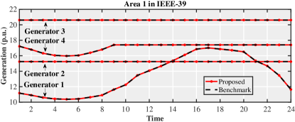
To verify the accuracy of the proposed distributed CC-OPF method, both IEEE test cases described in Section VI-A are used, where for each case is set to 24 to simulate the day-ahead dispatch. We compare the results of the proposed method to its benchmark, i.e., solving in a centralized manner with access to the global information.
Fig. 1 shows the generator outputs obtained by the proposed and benchmark methods. Due to space limitation, only the generator outputs in area 1 from the IEEE 39-bus system is shown in this figure, where generators 2 and 3 reach their maximal output from the very beginning and generator 4 hits its maximum from . As can be observed, the optimal solutions computed by the proposed method ideally coincide with the corresponding benchmarks.
| Test Case | Benchmark | Proposed Method | Relative Error |
|---|---|---|---|
| IEEE-39 | 110958.06 | 110958.13 | 6.03 |
| IEEE-118 | 8799.39124 | 8799.39122 | 2.12 |
| Test Case | Benchmark | Proposed Method | ||||||
|---|---|---|---|---|---|---|---|---|
| Formulating | Solving | Total | Formulating and Encrypting | Sharing | Solving and Decrypting | Total | ||
| IEEE-39 | 5 | 0.74 | 1.38 | 2.12 | 5.93 | 1.72 | 3.29 | 10.94 |
| IEEE-118 | 9 | 6.11 | 24.84 | 30.95 | 51.16 | 45.78 | 145.07 | 242.01 |
Further, the optimal objective function values obtained by the proposed method and its benchmark are listed in Table III for both test cases. To avoid repetitive illustration, only the objective function values obtained by ISO 1 using the proposed method are shown. Table III indicates that, the proposed method has very high accuracy — yielding relative errors of less than . These small deviations might be all numerical, yet they might also be caused by other possible reasons, e.g.,
-
1.
Although the encrypted problem is proved to be equivalent to mathematically, they might be different from the view of commercial solvers. For example, most of the constraints in are uncoupled, while the encryption tightly couples the constraints in . As a result, the commercial solver can easily identify and eliminate redundant constraints in before solving it, but fails to identify redundant constraint in . This may lead to different start points when solving and , thereby possibly yielding slightly different final solutions.
-
2.
The information exchange between ISOs is realized by the consensus-based algorithms, whose asymptotic convergence properties may introduce small error into the final results.
To verify the efficiency of the proposed distributed CC-OPF method, the computational time of each step in this method is measured and summarized in Table IV. Note that for the formulating, encrypting, and sharing steps, the time indicated is the overall computational time incurred by all ISOs, as they need cooperation to accomplish these steps. However, for the solving and decrypting steps, the time indicated is the maximal computational time incurred by an individual ISO, because these steps can be conducted by each ISO independently. The time consumed by the benchmark method is also listed in Table IV. This Table shows that the total computational time of the proposed method is always greater than that of its benchmark. Apparently, this is the price for enabling the distributed and confidentiality-preserving features. Nevertheless, the resulting overhead is acceptable for day-ahead dispatches.
VII Conclusion
This paper proposes a confidentiality-preserving distributed CC-OPF method on the basis of the TE technique. To this end, this paper first proves the TE technique’s adaptability to quadratic programming. Then, a fast distributed method for solving linear equation systems is developed, which enables regional ISOs to compute the coupled coefficients in chance constraints when they do not have the global information. Finally, the distributed CC-OPF method with confidentiality preservation is proposed. This distributed method can ensure that regional ISOs obtain and only obtain the accurate optimal dispatchable generations within their own regions without disclosing their confidential data.
References
- [1] H. L. van Soest, M. G. J. den Elzen, and D. P. van Vuuren, “Net-zero emission targets for major emitting countries consistent with the Paris Agreement,” Nature Communications, vol. 12, no. 1, p. 2140, 2021. [Online]. Available: https://doi.org/10.1038/s41467-021-22294-x
- [2] L. Wu, “A transformation-based multi-area dynamic economic dispatch approach for preserving information privacy of individual areas,” IEEE Transactions on Smart Grid, vol. 10, no. 1, pp. 722–731, 2019.
- [3] L. Roald and G. Andersson, “Chance-constrained ac optimal power flow: Reformulations and efficient algorithms,” IEEE Transactions on Power Systems, vol. 33, no. 3, pp. 2906–2918, 2018.
- [4] M. Lubin, Y. Dvorkin, and S. Backhaus, “A Robust Approach to Chance Constrained Optimal Power Flow With Renewable Generation,” IEEE Transactions on Power Systems, vol. 31, no. 5, pp. 3840–3849, Sep. 2016.
- [5] L. Roald, S. Misra, T. Krause, and G. Andersson, “Corrective Control to Handle Forecast Uncertainty: A Chance Constrained Optimal Power Flow,” IEEE Transactions on Power Systems, vol. 32, no. 2, pp. 1626–1637, Mar. 2017.
- [6] Y. Zhang, S. Shen, and J. L. Mathieu, “Distributionally Robust Chance-Constrained Optimal Power Flow With Uncertain Renewables and Uncertain Reserves Provided by Loads,” IEEE Transactions on Power Systems, vol. 32, no. 2, pp. 1378–1388, Mar. 2017.
- [7] J. Schmidli, L. Roald, S. Chatzivasileiadis, and G. Andersson, “Stochastic AC optimal power flow with approximate chance-constraints,” in 2016 IEEE Power and Energy Society General Meeting (PESGM), Jul. 2016, pp. 1–5.
- [8] M. Lubin, Y. Dvorkin, and L. Roald, “Chance Constraints for Improving the Security of AC Optimal Power Flow,” IEEE Transactions on Power Systems, vol. 34, no. 3, pp. 1908–1917, May 2019, arXiv: 1803.08754.
- [9] K. Baker and B. Toomey, “Efficient relaxations for joint chance constrained AC optimal power flow,” Electric Power Systems Research, vol. 148, pp. 230–236, Jul. 2017.
- [10] K. Baker and A. Bernstein, “Joint Chance Constraints in AC Optimal Power Flow: Improving Bounds through Learning,” IEEE Transactions on Smart Grid, pp. 1–1, 2019.
- [11] M. Jia, G. Hug, and C. Shen, “Iterative decomposition of joint chance constraints in opf,” IEEE Transactions on Power Systems, pp. 1–1, 2021.
- [12] A. Pena-Ordieres, D. K. Molzahn, L. Roald, and A. Waechter, “Dc optimal power flow with joint chance constraints,” IEEE Trans. Power Syst., pp. 1–1, 2020.
- [13] Z. Wang, C. Shen, F. Liu, X. Wu, C. Liu, and F. Gao, “Chance-Constrained Economic Dispatch With Non-Gaussian Correlated Wind Power Uncertainty,” IEEE Transactions on Power Systems, vol. 32, no. 6, pp. 4880–4893, Nov. 2017.
- [14] F. Ge, Y. Ju, Z. Qi, and Y. Lin, “Parameter Estimation of a Gaussian Mixture Model for Wind Power Forecast Error by Riemann L-BFGS Optimization,” IEEE Access, vol. 6, pp. 38 892–38 899, 2018.
- [15] Z. Wang, C. Shen, F. Liu, J. Wang, and X. Wu, “An Adjustable Chance-Constrained Approach for Flexible Ramping Capacity Allocation,” IEEE Transactions on Sustainable Energy, vol. 9, no. 4, pp. 1798–1811, Oct. 2018.
- [16] S. Mao, Y. Tang, Z. Dong, K. Meng, Z. Y. Dong, and F. Qian, “A privacy preserving distributed optimization algorithm for economic dispatch over time-varying directed networks,” IEEE Transactions on Industrial Informatics, vol. 17, no. 3, pp. 1689–1701, 2021.
- [17] M. Adibi and J. v. d. Woude, “Distributed learning control for economic power dispatch: A privacy preserved approach,” in 2020 IEEE 29th International Symposium on Industrial Electronics (ISIE), 2020, pp. 821–826.
- [18] P.J.M. Amended. (2017) Restated operating agreement of pjm interconnection. Brussels. [Online]. Available: http://pjm.com/-/media/documents/agreements/oa.ashx
- [19] P.J.M. (2014) Generator operational requirements: Generator data confidentiality procedures. [Online]. Available: https://pjm.com/~/media/committees-groups/committees/oc/20140818/20140818-m14d-section-11-revisions-red-lined-version.ashx
- [20] S. Sridhar and M. Govindarasu, “Model-based attack detection and mitigation for automatic generation control,” IEEE Transactions on Smart Grid, vol. 5, no. 2, pp. 580–591, 2014.
- [21] Y. Liu, P. Ning, and M. K. Reiter, “False data injection attacks against state estimation in electric power grids,” ACM Transactions on Information and System Security (TISSEC), vol. 14, no. 1, pp. 1–33, 2011.
- [22] K. Chatterjee, V. Padmini, and S. Khaparde, “Review of cyber attacks on power system operations,” in 2017 IEEE Region 10 Symposium (TENSYMP). IEEE, 2017, pp. 1–6.
- [23] A. Ahmadi-Khatir, A. J. Conejo, and R. Cherkaoui, “Multi-area unit scheduling and reserve allocation under wind power uncertainty,” IEEE Transactions on Power Systems, vol. 29, no. 4, pp. 1701–1710, 2014.
- [24] Z. Li, W. Wu, B. Zhang, and B. Wang, “Decentralized multi-area dynamic economic dispatch using modified generalized benders decomposition,” IEEE Transactions on Power Systems, vol. 31, no. 1, pp. 526–538, 2016.
- [25] H. Li, Z. Tan, and W. Li, “Privacy-preserving vertically partitioned linear program with nonnegativity constraints,” Optimization Letters, vol. 7, no. 8, pp. 1725–1731, 2013.
- [26] W. Li, H. Li, and C. Deng, “Privacy-preserving horizontally partitioned linear programs with inequality constraints,” Optimization Letters, vol. 7, no. 1, pp. 137–144, 2013.
- [27] Z. Li and M. Shahidehpour, “Privacy-preserving collaborative operation of networked microgrids with the local utility grid based on enhanced benders decomposition,” IEEE Transactions on Smart Grid, vol. 11, no. 3, pp. 2638–2651, 2020.
- [28] Y. Zhao, J. Yu, M. Ban, Y. Liu, and Z. Li, “Privacy-preserving economic dispatch for an active distribution network with multiple networked microgrids,” IEEE Access, vol. 6, pp. 38 802–38 819, 2018.
- [29] Z. Shi, H. Liang, S. Huang, and V. Dinavahi, “Distributionally robust chance-constrained energy management for islanded microgrids,” IEEE Transactions on Smart Grid, vol. 10, no. 2, pp. 2234–2244, 2019.
- [30] T. Guesmi, A. Farah, I. Marouani, B. Alshammari, and H. H. Abdallah, “Chaotic sine–cosine algorithm for chance-constrained economic emission dispatch problem including wind energy,” IET Renewable Power Generation, vol. 14, no. 10, pp. 1808–1821, 2020.
- [31] Y. Wang, S. Zhao, Z. Zhou, A. Botterud, Y. Xu, and R. Chen, “Risk adjustable day-ahead unit commitment with wind power based on chance constrained goal programming,” IEEE Trans. Sustain. Energy, vol. 8, no. 2, pp. 530–541, 2017.
- [32] J. Yang, N. Zhang, C. Kang, and Q. Xia, “A state-independent linear power flow model with accurate estimation of voltage magnitude,” IEEE Transactions on Power Systems, vol. 32, no. 5, pp. 3607–3617, 2017.
- [33] H. Shuai, J. Fang, X. Ai, Y. Tang, J. Wen, and H. He, “Stochastic optimization of economic dispatch for microgrid based on approximate dynamic programming,” IEEE Transactions on Smart Grid, vol. 10, no. 3, pp. 2440–2452, May 2019.
- [34] J. Zhan, W. Liu, and C. Y. Chung, “Stochastic transmission expansion planning considering uncertain dynamic thermal rating of overhead lines,” IEEE Transactions on Power Systems, vol. 34, no. 1, pp. 432–443, Jan 2019.
- [35] N. Azizan-Ruhi, F. Lahouti, A. S. Avestimehr, and B. Hassibi, “Distributed solution of large-scale linear systems via accelerated projection-based consensus,” IEEE Transactions on Signal Processing, vol. 67, no. 14, pp. 3806–3817, 2019.
- [36] T. C. Aysal, B. N. Oreshkin, and M. J. Coates, “Accelerated distributed average consensus via localized node state prediction,” IEEE Transactions on signal processing, vol. 57, no. 4, pp. 1563–1576, 2008.
- [37] M. Jia, Y. Wang, C. Shen, and G. Hug, “Privacy-preserving distributed clustering for electrical load profiling,” IEEE Transactions on Smart Grid, vol. 12, no. 2, pp. 1429–1444, 2021.