Change-point Detection for Sparse and Dense Functional Data in General Dimensions

Detailed model assumptions imposed on model (1) are collected in 1. For notational simplicity, without loss of generality, we set the general $d$-dimensional domain $\mathcal{D}$ to be $[0,1]^{d}$, as the results apply to any $\mathcal{D}$ that is homeomorphic to $[0,1]^{d}$.

1a allows the functional data to be observed on discrete grids and moreover, we allow for different grids at different time points. The sampling distribution $\mu$ is required to be lower bounded on the support $[0,1]^{d}$, which is a standard assumption widely used in the nonparametric literature (e.g. Tsybakov, 2009). Here, different functional curves are assumed to have the same number of grid points $n$. We remark that this is made for presentation simplicity only. It can indeed be further relaxed and the main results below will then depend on both the minimum and maximum numbers of grid points.

Note that 1a does not impose any restriction between the sampling frequency $n$ and the number of functional curves $T$, and indeed our method can handle both the dense case where $n\gg T$ and the sparse case where $n$ can be upper bounded by a constant. Besides the random sampling scheme studied here, another commonly studied scenario is the fixed design, where it usually assumes that the sampling locations $\{x_{i}\}_{i=1}^{n}$ are common to all functional curves across time. We remark that while we focus on the random design here, our proposed algorithm can be directly applied to the fixed design case without any modification. Furthermore, its theoretical justification under the fixed design case can be established similarly with minor modifications, which is omitted.

The observed functional data have mean functions $\{f^{*}_{t}\}_{t=1}^{T}$, which are assumed to be Hölder continuous in 1b. Note that the Hölder parameters in 1a and b are both denoted by $r$. We remark that different smoothness are allowed and we use the same $r$ here for notational simplicity. This sequence of mean functions is our primary interest and is assumed to possess a piecewise constant pattern, with the minimal spacing $\Delta$ being of the same order as $T$. This assumption essentially requires that the number of change-points is upper bounded. It can also be further relaxed and we will have more elaborated discussions on this matter in Section 5.

Our model allows for two sources of noise - functional noise and measurement error, which are detailed in 1c and d, respectively. Both the functional noise and the measurement error are allowed to possess temporal dependence and heavy-tailedness. For temporal dependence, we adopt the physical dependence framework by Wu (2005), which covers a wide range of time series models, such as ARMA and vector AR models. It further covers popular functional time series models such as functional AR and MA models (Hörmann and Kokoszka, 2010). We also remark that 1c and d impose a short range dependence, which is characterized by the absolute upper bounds $C_{\xi,2}$ and $C_{\delta,2}$. Further relaxation is possible by allowing the upper bounds $C_{\xi,2}$ and $C_{\delta,2}$ to vary with the sample size $T$.

The heavy-tail behavior is encoded in the parameter $q$. In 1c and d, we adopt the same quantity $q$ for presentational simplicity and remark that different heavy-tailedness levels are allowed. An extreme example is that when $q=\infty$, the noise is essentially sub-Gaussian. Importantly, 1d does not impose any restriction on the cross-sectional dependence among measurement errors observed on the same time $t$, which can be even perfectly correlated.

To estimate the change-point $\{\eta_{k}\}_{k=1}^{K}$ in the mean functions $\{f^{*}_{t}\}_{t=1}^{T}$, we propose a kernel-based cumulative sum (CUSUM) statistic, which is simple, intuitive and computationally efficient. The key idea is to recover the unobserved $\{f^{*}_{t}\}_{t=1}^{T}$ from the observations $\{(x_{t,i},y_{t,i})\}_{t=1,i=1}^{T,n}$ based on kernel estimation.

Given a kernel function $K(\cdot):\mathbb{R}^{d}\to\mathbb{R}^{+}$ and a bandwidth parameter $h>0$, we define $K_{h}(x)=h^{-d}K(x/h)$ for $x\in\mathbb{R}^{d}.$ Given the random grids $\{x_{t,i}\}_{t=1,i=1}^{T,n}$ and a bandwidth parameter $\bar{h}$, we define the density estimator of the sampling distribution $u(x)$ as

Given $\hat{p}(x)$ and a bandwidth parameter $h>0$, for any time $t=1,2,\cdots,T$, we define the kernel-based estimation for $f_{t}^{*}(x)$ as

Based on the kernel estimation $F_{t,h}(x)$, for any integer pair $0\leq s<e\leq T$, we define the CUSUM statistic as

The CUSUM statistic defined in (3) is the cornerstone of our algorithm and is based on two kernel estimators $\hat{p}(\cdot)$ and $F_{t,h}(\cdot)$. At a high level, the CUSUM statistic $\widetilde{F}_{t,h}^{(s,e]}(\cdot)$ estimates the difference in mean between the functional data in the time intervals $(s,t]$ and $(t,e]$. In the functional data analysis literature, other popular approaches for mean function estimation are reproducing kernel Hilbert space based methods and local polynomial regression. However, to our best knowledge, existing works based on the two approaches typically require that the functional data are temporally independent and it is not obvious how to extend their theoretical guarantees to the temporal dependence case. We therefore choose the kernel estimation method owing to its flexibility in terms of both methodology and theory and we derive new theoretical results on kernel estimation for functional data under temporal dependence and heavy-tailedness.

For multiple change-point estimation, a key ingredient is to isolate each single change-point with well-designed intervals in $[0,T]$. To achieve this, we combine the CUSUM statistic in (3) with a modified version of the seeded binary segmentation (SBS) proposed in Kovács et al. (2020). SBS is based on a collection of deterministic intervals defined in Definition 1.

The essential idea of the seeded intervals defined in Definition 1 is to provide a multi-scale system of searching regions for multiple change-points. SBS is computationally efficient with a computational cost of the order $O\{T\log(T)\}$ (Kovács et al., 2020).

Based on the CUSUM statistic and seeded intervals, Algorithm 1 summarises the proposed functional seeded binary segmentation algorithm (FSBS) for multiple change-point estimation in sequentially observed functional data. There are three main tuning parameters involved in Algorithm 1, the kernel bandwidth $\bar{h}$ in the estimation of the sampling distribution, the kernel bandwidth $h$ in the estimation of the mean function and the threshold parameter $\tau$ for declaring change-points. Their theoretical and numerical guidance will be presented in Sections 3.1 and 4, respectively.

Algorithm 1 is conducted in an iterative way, starting with the whole time course, using the multi-scale seeded intervals to search for the point according to the largest CUSUM value. A change-point is declared if the corresponding maximum CUSUM value exceeds a pre-specified threshold $\tau$ and the whole sequence is then split into two with the procedure being carried on in the sub-intervals.

Algorithm 1 utilizes a collection of random grid points $\{u_{m}\}_{m=1}^{\lceil\log(T)\rceil}\subseteq\{x_{t,i}\}_{t=1,i=1}^{T,n}$ to detect changes in the functional data. For a change of mean functions at the time point $\eta$ with $\|f^{*}_{\eta+1}-f^{*}_{\eta}\|_{\infty}>0$, we show in the appendix that, as long as $\lceil\log(T)\rceil$ grid points are sampled, with high probability, there is at least one point $u_{m^{\prime}}\in\{u_{m}\}_{m=1}^{\lceil\log(T)\rceil}$ such that $|f^{*}_{\eta+1}(u_{m^{\prime}})-f^{*}_{\eta}(u_{m^{\prime}})|\asymp\|f^{*}_{\eta+1}-f^{*}_{\eta}\|_{\infty}.$ Thus, this procedure allows FSBS to detect changes in the mean functions without evaluating functions on a dense lattice grid and thus improves computational efficiency.

We begin by imposing assumptions on the kernel function $K(\cdot)$ used in FSBS.

2 is a standard assumption in the nonparametric literature, see Giné and Guillou (1999, 2001), Kim et al. (2019), Wang et al. (2019) among many others. These assumptions hold for most commonly used kernels, including uniform, polynomial and Gaussian kernels.

Recall the minimal spacing $\Delta=\min_{k=1}^{K+1}(\eta_{k}-\eta_{k-1})$ defined in 1b. We further define the jump size at the $k$th change-point as $\kappa_{k}=\|f^{*}_{\eta_{k}+1}-f^{*}_{\eta_{k}}\|_{\infty}$ and define $\kappa=\min_{k=1}^{K}$ as the minimal jump size. 3 below details how strong the signal needs to be in terms of $\kappa$ and $\Delta$, given the grid size $n$, the number of functional curves $T$, smoothness parameter $r$, dimensionality $d$ and moment condition $q$.

We are now ready to present the main theorem, showing the consistency of FSBS.

In view of 3 and Theorem 1, we see that with properly chosen tuning parameters and with probability tending to one as the sample size $T$ grows, the output of FSBS estimates the correct number of change-points and

where the last inequality follows from 3. The above inequality shows that there exists a one-to-one mapping from $\{\widehat{\eta}_{k}\}_{k=1}^{K}$ to $\{\eta_{k}\}_{k=1}^{K}$, assigning by the smallest distance.

From sparse to dense regimes. In our setup, each curve is only observed at $n$ discrete points and we allow the full range of choices of $n$, representing from sparse to dense scenarios, all accompanied with consistency results. In the most sparse case $n=1$, 3 reads as $\kappa\sqrt{\Delta}\gtrsim T^{d/(4r+2d)}\times$ a logarithmic factor, under which the localisation error is upper bounded by $T^{d/(2r+d)}\kappa^{-2}$, up to a logarithmic factor. To the best of our knowledge, this challenging case has not been dealt in the existing change-point detection literature for functional data. In the most dense case, we can heuristically let $n=\infty$ and for simplicity let $q=\infty$ representing the sub-Gaussian noise case. 3 reads as $\kappa\sqrt{\Delta}\asymp\log^{1/2}(T)$ and the localisation error is upper bounded by $\kappa^{-2}\log(T)$. Both the SNR ratio and localisation error are the optimal rate in the univariate mean change-point localisation problem (Wang et al., 2020), implying the optimality of FSBS in the dense situation.

Tuning parameters. There are three tuning parameters involved. In the CUSUM statistic (3), we specify that the density estimator of the sampling distribution is a kernel estimator with bandwidth $\bar{h}\asymp(Tn)^{-1/(2r+d)}$. Due to the independence of the observation grids, such a choice of the bandwidth follows from the classical nonparametric literature (e.g. Tsybakov, 2009) and is minimax-rate optimal in terms of the estimation error. For completeness, we include the study of $\hat{p}(\cdot)$’s theoretical properties in Appendix B. In practice, there exist different default methods for the selection of $\bar{h}$ , see for example the function Hpi from the R package ks (Chacón and Duong (2018)).

The other bandwidth tuning parameter $h$ is also required to be $h\asymp(Tn)^{-1/(2r+d)}$. Despite that we allow for physical dependence in both functional noise and measurement error, we show that the same order of bandwidth (as $\bar{h}$) is required under 1. This is an interesting finding, if not surprising. This particular choice of $h$ is due to the fact that the physical dependence put forward by Wu (2005) is a short range dependence condition and does not change the rate of the sample size.

The threshold tuning parameter $\tau$ is set to be a high-probability upper bound on the CUSUM statistics when there is no change-point and is in fact of the form

This also reflects the requirement on the SNR detailed in 3, that $\kappa\sqrt{\Delta}\gtrsim\tau$.

Phase transition. Recall that the number of curves is $T$ and the number of observations on each curve is $n$. The asymptotic regime we discuss is to let $T$ diverge, while allowing all other parameters, including $n$, to be functions of $T$. In Theorem 1, we allow a full range of cases in terms of the relationship between $n$ and $T$. As a concrete example, when the smooth parameter $r=2$, the jump size $\kappa\asymp 1$ and in the one-dimensional case $d=1$, with high probability (ignoring logarithmic factors for simplicity),

This relationship between $n$ and $T$ was previously demonstrated in the mean function estimation literature (e.g. Cai and Yuan, 2011; Zhang and Wang, 2016), where the observations are discretely sampled from independently and identically distributed functional data. It is shown that the minimax estimation error rate also possesses the same phase transition between $n$ and $T$, i.e. with the transition boundary $n\asymp T^{1/4}$, which agrees with our finding under the change-point setting.

Physical dependence and heavy-tailedness In 1c and d, we allow for physical dependence type temporal dependence and heavy-tailed additive noise. As we have discussed, since the physical dependence is in fact a short range dependence, all the rates involved are the same as those in the independence cases, up to logarithmic factors. Having said this, the technical details required in dealing with this short range dependence are fundamentally different from those in the independence cases. From the result, it might be more interesting to discuss the effect of the heavy-tail behaviours, which are characterised by the parameter $q$. It can be seen from the rates in 3 and Theorem 1 that the effect of $q$ disappears and it behaves the same as if the noise is sub-Gaussian when $q\geq 10$.

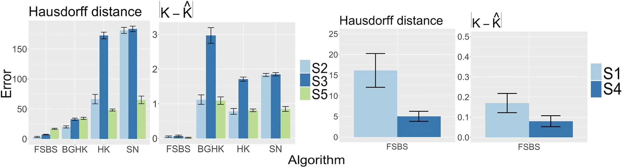
We compare the proposed FSBS with state-of-the-art methods for change-point detection in functional data across a wide range of simulation settings. The implementations for our approaches can be found at https://github.com/cmadridp/FSBS. We compare with three competitors: BGHK in Berkes et al. (2009), HK in Hörmann and Kokoszka (2010) and SN in Zhang et al. (2011). All three methods estimate change-points via examining mean change in the leading functional principal components of the observed functional data. BGHK is designed for temporally independent data while HK and SN can handle temporal dependence via the estimation of long-run variance and the use of self-normalization principle, respectively. All three methods require fully observed functional data. In practice, they convert discrete data to functional observations by using B-splines with 20 basis functions.

For the implementation of FSBS, we adopt the Gaussian kernel. Following the standard practice in kernel density estimation, the bandwidth $\bar{h}$ is selected by the function Hpi in the R package ks (Chacón and Duong (2018)). The tuning parameter $\tau$ and the bandwidth $h$ are chosen by cross-validation, with evenly-indexed data being the training set and oddly-indexed data being the validation set. For each pair of candidate $(h,\tau)$, we obtain change-point estimators $\{\widehat{\eta}_{k}\}_{k=1}^{\widehat{K}}$ on the training set and compute the validation loss $\sum_{k=1}^{\widehat{K}}\sum_{t\in[\widehat{\eta}_{k},\widehat{\eta}_{k+1})}\sum_{i=1}^{n}\{(\widehat{\eta}_{k+1}-\widehat{\eta}_{k})^{-1}\sum_{t=\widehat{\eta}_{k}+1}^{\widehat{\eta}_{k+1}}F_{t,h}(x_{t,i})-y_{t,i}\}^{2}.$ The pair $(h,\tau)$ is then chosen to be the one corresponding to the lowest validation loss.

We consider five different scenarios for the observations $\{x_{ti},y_{ti}\}_{t=1,i=1}^{T,n}$. For all scenarios 1-5, we set $T=200.$ Given the dimensionality $d$, denote a generic grid point as $x=(x^{(1)},\cdots,x^{(d)})$. Scenarios 1 to 4 are generated based on model (1). The basic setting is as follows.

$\bullet$ Scenario 1 (S1) Let $(n,d)=(1,1)$, the unevenly-spaced change-points be $(\eta_{1},\eta_{2})=(30,130)$ and the three distinct mean functions be $6\cos(\cdot)$, $6\sin(\cdot)$ and $6\cos(\cdot)$.

$\bullet$ Scenario 2 (S2) Let $(n,d)=(10,1)$, the unevenly-spaced change-points be $(\eta_{1},\eta_{2})=(30,130)$ and the three distinct mean functions be $2\cos(\cdot)$, $2\sin(\cdot)$ and $2\cos(\cdot)$.

$\bullet$ Scenario 3 (S3) Let $(n,d)=(50,1)$, the unevenly-spaced change-points be $(\eta_{1},\eta_{2})=(30,130)$ and the three distinct mean functions be $\cos(\cdot)$, $\sin(\cdot)$ and $\cos(\cdot)$.

$\bullet$ Scenario 4 (S4) Let $(n,d)=(10,2)$, the unevenly-spaced change-points be $(\eta_{1},\eta_{2})=(100,150)$ and the three distinct mean functions be $0$, $3x^{(1)}x^{(2)}$ and $0$.

For S1-S4, the functional noise is generated as $\xi_{t}(x)=0.5\xi_{t-1}(x)+\sum_{i=1}^{50}i^{-1}b_{t,i}h_{i}(x)$, where $\{h_{i}(x)=\prod_{j=1}^{d}(1/\sqrt{2})\pi\sin(ix^{(j)})\}_{i=1}^{50}$ are basis functions and $\{b_{t,i}\}_{t=1,i=1}^{T,50}$ are i.i.d. standard normal random variables. The measurement error is generated as $\delta_{t}=0.3\delta_{t-1}+\epsilon_{t}$, where $\{\epsilon_{t}\}_{t=1}^{T}$ are i.i.d. $\mathcal{N}(0,0.5I_{n})$. We observe the noisy functional data $\{y_{ti}\}_{t=1,i=1}^{T,n}$ at grid points $\{x_{ti}\}_{t=1,i=1}^{T,n}$ independently sampled from $\mathrm{Unif}([0,1]^{d})$.

Scenario 5 is adopted from Zhang et al. (2011) for densely-sampled functional data without measurement error.

$\bullet$ Scenario 5 (S5) Let $(n,d)=(50,1)$, the evenly-spaced change-points be $(\eta_{1},\eta_{2})=(68,134)$ and the three distinct mean functions be 0, $\sin(\cdot)$ and $2\sin(\cdot)$.

The grid points $\{x_{ti}\}_{i=1}^{50}$ are $50$ evenly-spaced points in $[0,1]$ for all $t=1,\cdots,T$. The functional noise is generated as $\xi_{t}(\cdot)=\int_{[0,1]}\psi(\cdot,u)\xi_{t-1}(u)\,\mathrm{d}u+\epsilon_{t}(\cdot)$, where $\{\epsilon_{t}(\cdot)\}_{t=1}^{T}$ are independent standard Brownian motions and $\psi(v,u)=1/3\exp((v^{2}+u^{2})/2)$ is a bivariate Gaussian kernel.

S1-S5 represent a wide range of simulation settings including the extreme sparse case S1, sparse case S2, the two-dimensional domain case S4, and the densely sampled cases S3 and S5. Note that S1 and S4 can only be handled by FSBS as for S1 it is impossible to estimate a function via B-spline based on one point and for S4, the domain is of dimension 2.

Evaluation result: For a given set of true change-points $\mathcal{C}=\{\eta_{k}\}_{k=1}^{K}$, we evaluate the accuracy of the estimator $\{\widehat{\eta}_{k}\}_{k=1}^{\widehat{K}}$ by the difference $|\widehat{K}-K|$ and the Hausdorff distance $d(\hat{\mathcal{C}},\mathcal{C})$, defined by $d(\hat{\mathcal{C}},\mathcal{C})=\max\{\max_{x\in{\hat{\mathcal{C}}}}\min_{y\in{\mathcal{C}}}\{|x-y|\},\max_{y\in{\hat{\mathcal{C}}}}\min_{x\in{\mathcal{C}}}\{|x-y|\}\}$. For $\hat{\mathcal{C}}=\varnothing$, we use the convention that $|\widehat{K}-K|=K$ and $d(\hat{\mathcal{C}},\mathcal{C})=T$.

For each scenario, we repeat the experiments 100 times and Figure 1 summarizes the performance of FSBS, BGHK, HK and SN. Tabulated results can be found in Appendix A. As can be seen, FSBS consistently outperforms the competing methods by a wide margin and demonstrates robust behaviour across the board for both sparsely and densely sampled functional data.

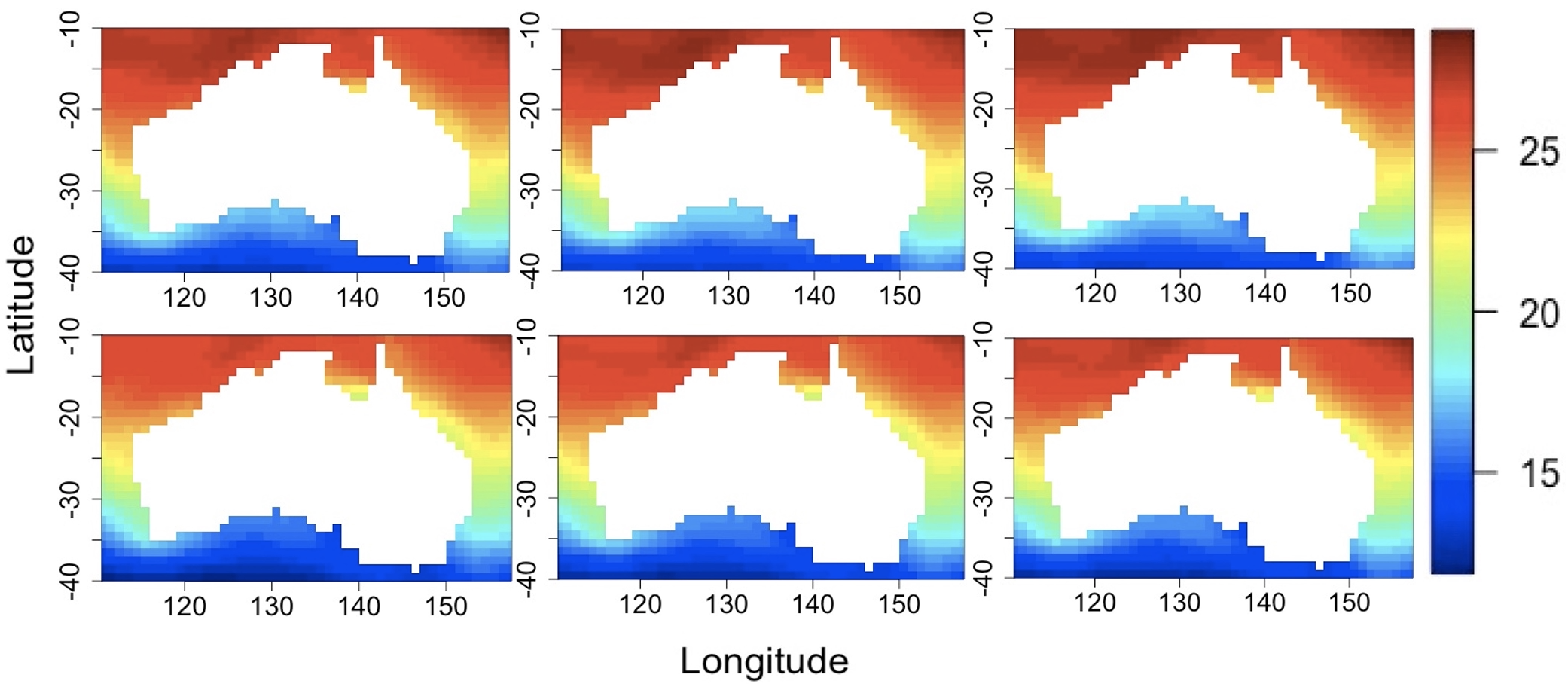
We consider the COBE-SSTE dataset (Physical Sciences Laboratory, 2020), which consists of monthly average sea surface temperature (SST) from 1940 to 2019, on a $1$ degree latitude by $1$ degree longitude grid $(48\times 30)$ covering Australia. The specific coordinates are latitude $10$S-$39$S and longitude $110$E-$157$E.

We apply FSBS to detect potential change-points in the two-dimensional SST. The implementation of FSBS is the same as the one described in Section 4.1. To avoid seasonality, we apply FSBS to the SST for the month of June from 1940 to 2019. We further conduct the same analysis separately for the month of July for robustness check.

For both the June and July data, two change-points are identified by FSBS, Year 1981 and 1996, suggesting the robustness of the finding. The two change-points might be associated with years when both the Indian Ocean Dipole and Oceanic Niño Index had extreme events (Ashok et al., 2003). The El Niño/Southern Oscillation has been recognized as an important manifestation of the tropical ocean-atmosphere-land coupled system. It is an irregular periodic variation in winds and sea surface temperatures over the tropical eastern Pacific Ocean. Much of the variability in the climate of Australia is connected with this phenomenon (Australian Government, 2014).

To visualize the estimated change, Figure 2 depicts the average SST before the first change-point Year 1981, between the two change-points, and after the second change-point Year 1996. The two rows correspond to the June and July data, respectively. As we can see, the top left corners exhibit different patterns in the three periods, suggesting the existence of change-points.

References

- Ashok et al. (2003) Karumuri Ashok, Zhaoyong Guan, and Toshio Yamagat. A look at the relationship between the enso and the indian ocean dipole. Journal of the Meteorological Society of Japan. Ser. II, 81(1):41–56, 2003. doi: 10.2151/jmsj.81.41.
- Aue et al. (2009) Alexander Aue, Robertas Gabrys, Lajos Horváth, and Piotr Kokoszka. Estimation of a change-point in the mean function of functional data. Journal of Multivariate Analysis, 100(10):2254–2269, 2009.
- Aue et al. (2018) Alexander Aue, Gregory Rice, and Ozan Sönmez. Detecting and dating structural breaks in functional data without dimension reduction. Journal of the Royal Statistical Society: Series B (Statistical Methodology), 80(3):509–529, 2018.
- Australian Government (2014) Australian Government. What is El Niño and how does it impact Australia? http://www.bom.gov.au/climate/updates/articles/a008-el-nino-and-australia.shtml, June 2014.
- Berkes et al. (2009) István Berkes, Robertas Gabrys, Lajos Horváth, and Piotr Kokoszka. Detecting changes in the mean of functional observations. Journal of the Royal Statistical Society: Series B (Statistical Methodology), 71(5):927–946, 2009.
- Bonner et al. (2014) Simon J Bonner, Nathaniel K Newlands, and Nancy E Heckman. Modeling regional impacts of climate teleconnections using functional data analysis. Environmental and Ecological Statistics, 21(1):1–26, 2014.
- Cai and Yuan (2011) T Tony Cai and Ming Yuan. Optimal estimation of the mean function based on discretely sampled functional data: Phase transition. The Annals of Statistics, 39(5):2330–2355, 2011.
- Chacón and Duong (2018) José E Chacón and Tarn Duong. Multivariate kernel smoothing and its applications. Chapman and Hall/CRC, 2018.
- Chiou et al. (2014) Jeng-Min Chiou, Yi-Chen Zhang, Wan-Hui Chen, and Chiung-Wen Chang. A functional data approach to missing value imputation and outlier detection for traffic flow data. Transportmetrica B: Transport Dynamics, 2(2):106–129, 2014.
- Dai et al. (2019) Xiongtao Dai, Hans-Georg Müller, Jane-Ling Wang, and Sean CL Deoni. Age-dynamic networks and functional correlation for early white matter myelination. Brain Structure and Function, 224(2):535–551, 2019.
- Dette et al. (2020) Holger Dette, Kevin Kokot, and Stanislav Volgushev. Testing relevant hypotheses in functional time series via self-normalization. Journal of the Royal Statistical Society: Series B (Statistical Methodology), 82(3):629–660, 2020.
- Fan et al. (2014) Yingying Fan, Natasha Foutz, Gareth M James, and Wolfgang Jank. Functional response additive model estimation with online virtual stock markets. The Annals of Applied Statistics, 8(4):2435–2460, 2014.
- Fraiman et al. (2014) Ricardo Fraiman, Ana Justel, Regina Liu, and Pamela Llop. Detecting trends in time series of functional data: A study of antarctic climate change. Canadian Journal of Statistics, 42(4):597–609, 2014.
- Giné and Guillou (1999) Evarist Giné and Armelle Guillou. Laws of the iterated logarithm for censored data. The Annals of Probability, 27(4):2042–2067, 1999.
- Giné and Guillou (2001) Evarist Giné and Armelle Guillou. On consistency of kernel density estimators for randomly censored data: rates holding uniformly over adaptive intervals. Annales de l’IHP Probabilités et statistiques, 37(4):503–522, 2001.
- Giné and Guillou (2002) Evarist Giné and Armelle Guillou. Rates of strong uniform consistency for multivariate kernel density estimators. Annales de l’Institut Henri Poincare (B) Probability and Statistics, 38(6):907–921, 2002. ISSN 0246-0203. doi: https://doi.org/10.1016/S0246-0203(02)01128-7.
- Hörmann and Kokoszka (2010) Siegfried Hörmann and Piotr Kokoszka. Weakly dependent functional data. The Annals of Statistics, 38(3):1845–1884, 2010.
- Jiang (2017) Heinrich Jiang. Uniform convergence rates for kernel density estimation. In International Conference on Machine Learning, pages 1694–1703. PMLR, 2017.
- Kim et al. (2019) Jisu Kim, Jaehyeok Shin, Alessandro Rinaldo, and Larry Wasserman. Uniform convergence rate of the kernel density estimator adaptive to intrinsic volume dimension. In International Conference on Machine Learning, pages 3398–3407. PMLR, 2019.
- Kirch (2006) Claudia Kirch. Resampling methods for the change analysis of dependent data. PhD thesis, Universität zu Köln, 2006.
- Kovács et al. (2020) Solt Kovács, Housen Li, Peter Bühlmann, and Axel Munk. Seeded binary segmentation: A general methodology for fast and optimal change point detection. arXiv preprint arXiv:2002.06633, 2020.
- Liu et al. (2013) Weidong Liu, Han Xiao, and Wei Biao Wu. Probability and moment inequalities under dependence. Statistica Sinica, pages 1257–1272, 2013.
- Petersen et al. (2019) Alexander Petersen, Sean Deoni, and Hans-Georg Müller. Fréchet estimation of time-varying covariance matrices from sparse data, with application to the regional co-evolution of myelination in the developing brain. The Annals of Applied Statistics, 13(1):393–419, 2019.
- Physical Sciences Laboratory (2020) Physical Sciences Laboratory. COBE SST2 and Sea-Ice. https://psl.noaa.gov/data/gridded/data.cobe2.html, April 2020.
- Rigollet and Vert (2009) Philippe Rigollet and Régis Vert. Optimal rates for plug-in estimators of density level sets. Bernoulli, 15(4):1154–1178, 2009.
- Rinaldo and Wasserman (2010) Alessandro Rinaldo and Larry Wasserman. Generalized density clustering. The Annals of Statistics, 38(5):2678–2722, 2010.
- Sriperumbudur and Steinwart (2012) Bharath Sriperumbudur and Ingo Steinwart. Consistency and rates for clustering with dbscan. In Artificial Intelligence and Statistics, pages 1090–1098. PMLR, 2012.
- Tsybakov (2009) Alexandre B Tsybakov. Introduction to Nonparametric Estimation. Springer series in statistics. Springer, Dordrecht, 2009. doi: 10.1007/b13794.
- Vershynin (2018) Roman Vershynin. High-dimensional probability: An introduction with applications in data science, volume 47. Cambridge university press, 2018.
- Wang et al. (2019) Daren Wang, Xinyang Lu, and Alessandro Rinaldo. Dbscan: Optimal rates for density-based cluster estimation. Journal of Machine Learning Research, 2019.
- Wang et al. (2020) Daren Wang, Yi Yu, and Alessandro Rinaldo. Univariate mean change point detection: Penalization, cusum and optimality. Electronic Journal of Statistics, 14(1):1917–1961, 2020.
- Wang et al. (2016) Jane-Ling Wang, Jeng-Min Chiou, and Hans-Georg Müller. Functional data analysis. Annual Review of Statistics and Its Application, 3:257–295, 2016.
- Wu (2005) Wei Biao Wu. Nonlinear system theory: Another look at dependence. Proceedings of the National Academy of Sciences, 102(40):14150–14154, 2005.
- Zhang et al. (2011) Xianyang Zhang, Xiaofeng Shao, Katharine Hayhoe, and Donald J Wuebbles. Testing the structural stability of temporally dependent functional observations and application to climate projections. Electronic Journal of Statistics, 5:1765–1796, 2011.
- Zhang and Wang (2016) Xiaoke Zhang and Jane-Ling Wang. From sparse to dense functional data and beyond. The Annals of Statistics, 44(5):2281–2321, 2016.
Appendices
Appendix A Detailed simulation results
We present the tables containing the results of the simulation study in Section 4.1 of the main text.