Channel Estimation for RIS Assisted Wireless Communications: Part II - An Improved Solution Based on Double-Structured Sparsity
(Invited Paper)

We consider that the BS and the RIS respectively employ the $M$-antenna and the $N$-element uniform planer array (UPA) to simultaneously serve ${K}$ single-antenna users. Let $\bf{G}$ of size ${M\times N}$ denote the channel from the RIS to the BS, and ${\bf{h}}_{r,k}$ of size ${N\times 1}$ denote the channel from the ${k}$th user to the RIS $\left({k=1,2,\cdots,K}\right)$. The widely used Saleh-Valenzuela channel model is adopted to represent ${\bf{G}}$ as [5]

where $L_{G}$ represents the number of paths between the RIS and the BS, ${\alpha}^{G}_{l_{1}}$, $\vartheta^{G_{r}}_{l_{1}}$ (${\psi}^{G_{r}}_{l_{1}}$), and ${\vartheta}^{G_{t}}_{l_{1}}$ (${\psi}^{G_{t}}_{l_{1}}$) represent the complex gain consisting of path loss, the azimuth (elevation) angle at the BS, and the azimuth (elevation) angle at the RIS for the $l_{1}$th path. Similarly, the channel ${\bf{h}}_{r,k}$ can be represented by

where $L_{r,k}$ represents the number of paths between the $k$th user and the RIS, ${\alpha}^{r,k}_{l_{2}}$, $\vartheta^{r,k}_{l_{2}}$ (${\psi}^{r,k}_{l_{2}}$) represent the complex gain consisting of path loss, the azimuth (elevation) angle at the RIS for the $l_{2}$th path. ${\bf{b}}\left(\vartheta,\psi\right)\in{\mathbb{C}^{M\times 1}}$ and ${\bf{a}}\left(\vartheta,\psi\right)\in{\mathbb{C}^{N\times 1}}$ represent the normalized array steering vector associated to the BS and the RIS, respectively. For a typical $N_{1}\times N_{2}$ ($N=N_{1}\times N_{2}$) UPA, ${\bf{a}}\left(\vartheta,\psi\right)$ can be represented by [5]

where ${\bf{n}}_{1}=[0,1,\cdots,N_{1}-1]$ and ${\bf{n}}_{2}=[0,1,\cdots,N_{2}-1]$, $\lambda$ is the carrier wavelength, and $d$ is the antenna spacing usually satisfying $d=\lambda/2$.

Further, we denote ${\bf{H}}_{k}\triangleq{\bf{G}}{\rm{diag}}\left({\bf{h}}_{r,k}\right)$ as the $M\times N$ cascaded channel for the $k$th user. Using the virtual angular-domain representation, ${\bf{H}}_{k}\in\mathbb{C}^{M\times N}$ can be decomposed as

where ${\tilde{\bf{H}}}_{k}$ denotes the ${M\times N}$ angular cascaded channel, ${\bf{U}}_{M}$ and ${\bf{U}}_{N}$ are respectively the ${M\times M}$ and ${N\times N}$ dictionary unitary matrices at the BS and the RIS [5]. Since there are limited scatters around the BS and the RIS, the angular cascaded channel ${\tilde{\bf{H}}}_{k}$ has a few non-zero elements, which exhibits the sparsity.

In this paper, we assume that the direct channel between the BS and the user is known for BS, which can be easily estimated as these in conventional wireless communication systems [5]. Therefore, we only focus on the cascaded channel estimation problem.

By adopting the widely used orthogonal pilot transmission strategy, all users transmit the known pilot symbols to the BS via the RIS over ${Q}$ time slots for the uplink channel estimation. Specifically, in the ${q}$th $\left({q=1,2,\cdots,Q}\right)$ time slot, the effective received signal ${{\bf{y}}_{k,q}}\in\mathbb{C}^{M\times 1}$ at the BS for the $k$th user after removing the impact of the direct channel can be represented as

where $s_{k,q}$ is the pilot symbol sent by the $k$th user, ${\bm{\theta}}_{q}=[\theta_{q,1},\cdots,\theta_{q,N}]^{T}$ is the $N\times 1$ reflecting vector at the RIS with $\theta_{q,n}$ representing the reflecting coefficient at the $n$th RIS element $(n=1,\cdots,N)$ in the $q$th time slot, ${{\bf{w}}_{k,q}}\sim{\cal C}{\cal N}\left({0,\sigma^{2}{\bf{I}}_{M}}\right)$ is the ${{M}\times 1}$ received noise with ${\sigma^{2}}$ representing the noise power. According to the cascaded channel ${\bf{H}}_{k}={\bf{G}}{\rm{diag}}\left({\bf{h}}_{r,k}\right)$, we can rewrite (5) as

After ${Q}$ time slots of pilot transmission, we can obtain the ${M\times Q}$ overall measurement matrix ${\bf{Y}}_{k}={[{\bf{y}}_{k,1},\cdots,{\bf{y}}_{k,Q}]}$ by assuming ${s_{k,q}}=1$ as

where ${\bm{\Theta}}={[{\bm{\theta}}_{1},\cdots,{\bm{\theta}}_{Q}]}$ and ${\bf{W}}_{k}=[{\bf{w}}_{k,1},\cdots,{\bf{w}}_{k,Q}]$. By substituting (4) into (7), we can obtain

Let denote ${{\tilde{\bf{Y}}}_{k}}=\left({\bf{U}}_{M}^{H}{{\bf{Y}}_{k}}\right)^{H}$ as the $Q\times M$ effective measurement matrix, and ${{\tilde{\bf{W}}}_{k}}=\left({\bf{U}}_{M}^{H}{{\bf{W}}_{k}}\right)^{H}$ as the $Q\times M$ effective noise matrix, (7) can be rewritten as a CS model:

where ${{\tilde{\bf{\Theta}}}}=\left({\bf{U}}_{N}^{T}{{\bm{\Theta}}}\right)^{H}$ is the $Q\times N$ sensing matrix. Based on (9), we can respectively estimate the angular cascaded channel for each user $k$ by conventional CS algorithms, such as OMP algorithm. However, under the premise of ensuring the estimation accuracy, the pilot overhead required by the conventional CS algorithms is still high.

In order to further explore the sparsity of the angular cascaded channel both in row and column, the angular cascaded channel ${\tilde{\bf{H}}}_{k}$ in (4) can be expressed as

where both ${\tilde{\bf{b}}}\left(\vartheta,\psi\right)={\bf{U}}_{M}^{H}{\bf{b}}\left(\vartheta,\psi\right)$ and ${\tilde{\bf{a}}}\left(\vartheta,\psi\right)={\bf{U}}_{N}^{H}{{\bf{a}}}\left(\vartheta,\psi\right)$ have only one non-zero element, which lie on the position of array steering vector at the direction $\left(\vartheta,\psi\right)$ in ${\bf{U}}_{M}$ and ${\bf{U}}_{N}$. Based on (10), we can find that each complete reflecting path $(l_{1},l_{2})$ can provide one non-zero element for ${\tilde{\bf{H}}}_{k}$, whose row index depends on $\left(\vartheta^{G_{r}}_{l_{1}},\psi^{G_{r}}_{l_{1}}\right)$ and column index depends on $\left(\vartheta^{G_{t}}_{l_{1}}+\vartheta^{r,k}_{l_{2}},\psi^{G_{t}}_{l_{1}}+\psi^{r,k}_{l_{2}}\right)$. Therefore, ${\tilde{\bf{H}}}_{k}$ has $L_{G}$ non-zero rows, where each non-zero row has $L_{r,k}$ non-zero columns. The total number of non-zero elements is $L_{G}L_{r,k}$, which is usually much smaller than $MN$.

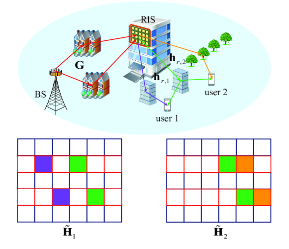
More importantly, we can find that different sparse channels $\{{\tilde{\bf{H}}}_{k}\}_{k=1}^{K}$ exhibit the double-structured sparsity, as shown in Fig. 1. Firstly, since different users communicate with the BS via the common RIS, the channel $\bf{G}$ from the RIS to the BS is common for all users. From (10), we can also find that $\bigg{\{}\left(\vartheta^{G_{r}}_{l_{1}},\psi^{G_{r}}_{l_{1}}\right)\bigg{\}}_{l_{1}=1}^{L_{G}}$ is independent of the user index $k$. Therefore, the non-zero elements of $\{{\tilde{\bf{H}}}_{k}\}_{k=1}^{K}$ lie on the completely common $L_{G}$ rows. Secondly, since different users will share part of the scatters between the RIS and users, $\{{\bf{h}}_{r,k}\}_{k=1}^{K}$ may enjoy partially common paths with the same angles at the RIS. Let $L_{c}$ (${L_{c}}\leq{L_{r,k}},\forall k$) denote the number of common paths for $\{{\bf{h}}_{r,k}\}_{k=1}^{K}$, then we can find that for $\forall l_{1}$, there always exists $\bigg{\{}\left(\vartheta^{G_{t}}_{l_{1}}-\vartheta^{r,k}_{l_{2}},\psi^{G_{t}}_{l_{1}}-\psi^{r,k}_{l_{2}}\right)\bigg{\}}_{l_{2}=1}^{L_{c}}$ shared by $\{{\tilde{\bf{H}}}_{k}\}_{k=1}^{K}$. That is to say, for each common non-zero rows $l_{1}$ ($l_{1}=1,2,\cdots,L_{G}$), $\{{\tilde{\bf{H}}}_{k}\}_{k=1}^{K}$ enjoy $L_{c}$ common non-zero columns. This double-structured sparsity of the angular cascaded channels can be summarized as follows from the perspective of row and column, respectively.

• •

  Row-structured sparsity: Let $\Omega_{r}^{k}$ denote the row set of non-zero elements for ${\tilde{\bf{H}}}_{k}$, then we have

  $$\Omega_{r}^{1}=\Omega_{r}^{2}=\cdots=\Omega_{r}^{K}=\Omega_{r},$$

  (11)

  where $\Omega_{r}$ represents the completely common row support for $\{{\tilde{\bf{H}}}_{k}\}_{k=1}^{K}$.

• •

  Partially column-structured sparsity: Let $\Omega_{c}^{l,k}$ denote the column set of non-zero elements for the $l_{1}$th non-zero row of ${\tilde{\bf{H}}}_{k}$, then we have

  $$\Omega_{c}^{l_{1},1}\cap\Omega_{c}^{l_{1},2}\cap\cdots\cap\Omega_{c}^{l_{1},K}=\Omega_{c}^{l_{1},{\rm{Com}}},\quad l_{1}=1,2,\cdots,L_{G},$$

  (12)

  where $\Omega_{c}^{{l,{\rm{Com}}}}$ represents the partially common column support for the $l_{1}$th non-zero row of $\{{\tilde{\bf{H}}}_{k}\}_{k=1}^{K}$.

Based on the above double-structured sparsity, the cascaded channels for different users can be jointly estimated to improve the channel estimation accuracy.

In this subsection, we propose the DS-OMP based cascaded channel estimation scheme by integrating the double-structured sparsity into the classical OMP algorithm. The specific algorithm can be summarized in Algorithm 1, which includes three key stages to detect supports of angular cascaded channels.

The main procedure of Algorithm 1 can be explained as follows. Firstly, the completely common row support $\Omega_{r}$ is jointly estimated thanks to the row-structured sparsity in Step 1, where $\Omega_{r}$ consists of $L_{G}$ row indexes associated with $L_{G}$ non-zero rows. Secondly, for the $l_{1}$th non-zero row, the partially common column support $\Omega_{c}^{l_{1},{\rm{Com}}}$ can be further jointly estimated thanks to the partially column-structured sparsity in Step 2. Thirdly, the user-specific column supports for each user $k$ can be individually estimated in Step 3. After detecting supports of all sparse matrices, we adopt the LS algorithm to obtain corresponding estimated matrices $\{{{\hat{\tilde{\bf{H}}}}_{k}}\}_{k=1}^{K}$ in Steps 4-8. It should be noted that the sparse signal in (9) is ${\tilde{\bf{H}}}_{k}^{H}$, thus the sparse matrix estimated by the LS algorithm in Step 6 is ${\hat{\tilde{\bf{H}}}}_{k}^{H}$. Finally, we can obtain the estimated cascaded channels $\{{{\hat{{\bf{H}}}}_{k}}\}_{k=1}^{K}$ by transforming angular channels into spatial channels in Step 9.

In the following part, we will introduce how to estimate the completely common row support, the partially common column supports, and the individual column supports for the first three stages in detail.

1) Stage 1: Estimating the completely common row support. Thanks to the row-structured sparsity of the angular cascaded channels, we can jointly estimate the completely common row support $\Omega_{r}$ for $\{{{{\tilde{\bf{H}}}}_{k}}\}_{k=1}^{K}$ by Algorithm 2.

From the virtual angular-domain channel representation (4), we can find that non-zero rows of $\{{{{\tilde{\bf{H}}}}_{k}}\}_{k=1}^{K}$ are corresponding to columns with high power in the received pilots $\{{{{\tilde{\bf{Y}}}}_{k}}\}_{k=1}^{K}$. Since $\{{{{\tilde{\bf{H}}}}_{k}}\}_{k=1}^{K}$ have the completely common non-zero rows, $\{{{{\tilde{\bf{Y}}}}_{k}}\}_{k=1}^{K}$ can be jointly utilized to estimate the completely common row support $\Omega_{r}$, which can resist the effect of noise. Specifically, we denote $\bf{g}$ of size $M\times 1$ to save the sum power of columns of $\{{{{\tilde{\bf{Y}}}}_{k}}\}_{k=1}^{K}$, as in Step 2 of Algorithm 2. Finally, $L_{G}$ indexes of elements with the largest amplitudes in $\bf{g}$ are selected as the estimated completely common row support ${\hat{\Omega}}_{r}$ in Step 4, where $\mathcal{T}({\bf{x}},L)$ denotes a prune operator on $\bf{x}$ that sets all but $L$ elements with the largest amplitudes to zero, and $\Gamma(\bf{x})$ denotes the support of ${\bf{x}}$, i.e., $\Gamma({\bf{x}})=\{i,{\bf{x}}(i)\neq 0\}$.

After obtaining $L_{G}$ non-zero rows by Algorithm 2, we focus on estimating the column support ${{\Omega}}_{c}^{l_{1},k}$ for each non-zero row $l_{1}$ and each user $k$ by the following Stage 2 and 3.

2) Stage 2: Estimating the partially common column supports. Thanks to the partially column-structured sparsity of the angular cascaded channels, we can jointly estimate the partially common column supports $\{{{{\Omega}}_{c}^{l_{1},{\rm{Com}}}}\}_{l_{1}=1}^{L}$ for $\{{{{\tilde{\bf{H}}}}_{k}}\}_{k=1}^{K}$ by Algorithm 3.

For the $l_{1}$th non-zero row, we only need to utilize the effective measurement vector ${\tilde{\bf{y}}}_{k}={{\tilde{\bf{Y}}}}_{k}(:,{\hat{\Omega}}_{r}(l_{1}))$ to estimate the partially common column support ${\Omega}_{c}^{l_{1},{\rm Com}}$. The basic idea is that, we firstly estimate the column support ${{\Omega}}_{c}^{l_{1},k}$ with $L_{r,k}$ indexes for each user $k$, then we select $L_{c}$ indexes associated with the largest number of times from all $\{{{\Omega}}_{c}^{l_{1},k}\}_{k=1}^{K}$ as the estimated partially common column support ${\hat{\Omega}}_{c}^{l_{1},{\rm{Com}}}$.

In order to estimate the column supports for each user $k$, the correlation between the sensing matrix ${\tilde{\bm{\Theta}}}$ and the residual vector ${\tilde{\bf{r}}}_{k}$ needs to be calculated. As shown in Step 5 of Algorithm 3, the most correlative column index in ${\tilde{\bm{\Theta}}}$ with ${\tilde{\bf{r}}}_{k}$ is regarded as the newly found column support index $n^{*}$. Based on the updated column support ${\hat{\Omega}}_{c}^{l_{1},k}$ in Step 6, the estimated sparse vector ${\hat{\tilde{\bf{h}}}}_{k}$ is obtained by using the LS algorithm in Step 8. Then, the residual vector ${\tilde{\bf{r}}}_{k}$ is updated by removing the effect of non-zero elements that have been estimated in Step 9. Particularly, the $N\times 1$ vector ${\bf{c}}^{l_{1}}$ is used to count the number of times for selected column indexes in Step 10. Finally, the $L_{c}$ indexes of elements with the largest value in ${\bf{c}}^{l_{1}}$ are selected as the estimated partially common column support ${\hat{\Omega}}_{c}^{l_{1},{\rm{Com}}}$ in Step 13.

3) Stage 3: Estimating the individual column supports. Based on the estimated completely common row support ${\hat{\Omega}}_{r}$ and the estimated partially common column supports $\{{\hat{\Omega}}_{c}^{l_{1},{\rm{Com}}}\}_{l_{1}=1}^{L}$, the column support ${{\Omega}}_{c}^{l_{1},k}$ for each non-zero row $l_{1}$ and each user $k$ can be estimated by Algorithm 4.

For the $l_{1}$th non-zero row, we have estimated $L_{c}$ column support indexes by Algorithm 3. Thus, there are $L_{r,k}-L_{c}$ user-specific column support indexes to be estimated for each user $k$. The column support ${\hat{\Omega}}_{c}^{l_{1},k}$ is initialized as ${\hat{\Omega}}_{c}^{l_{1},{\rm Com}}$. Based on ${\hat{\Omega}}_{c}^{l_{1},{\rm Com}}$, the estimated sparse vector ${\hat{\tilde{\bf{h}}}}_{k}$ and residual vector ${{\tilde{\bf{r}}}}_{k}$ are initialized in Step 5 and Step 6. Then, the column support ${\hat{\Omega}}_{c}^{l_{1},k}$ for $\forall l_{1}$ and $\forall k$ can be estimated in Steps 7-13 by following the same idea of Algorithm 3.

Through the above three stages, the supports of all angular cascaded channels are estimated by exploiting the double-structured sparsity. It should be pointed out that, if there are no common scatters between the RIS and users, the double-structured sparse channel will be simplified as the row-structured sparse channel. In this case, the cascaded channel estimation can also be solved by the proposed DS-OMP algorithm, where Stage 2 will be removed.

In this subsection, the computational complexity of the proposed DS-OMP algorithm is analyzed in terms of three stages of detecting supports. In Stage 1, the computational complexity mainly comes from Step 2 in Algorithm 2, which calculates the power of $M$ columns of ${\tilde{\bf{Y}}}_{k}$ of size $Q\times M$ for $k=1,2,\cdots,K$. The corresponding computational complexity is $\mathcal{O}(KMQ)$. In Stage 2, for each non-zero row $l_{1}$ and each user $k$ in Algorithm 3 , the computational complexity $\mathcal{O}(NQL_{r,k}^{3})$ is the same as that of OMP algorithm [6]. Considering $L_{G}K$ iterations, the overall computational complexity of Algorithm 3 is $\mathcal{O}(L_{G}KNQ{L}_{r,k}^{3})$. Similarly, the overall computational complexity of Algorithm 4 is $\mathcal{O}(L_{G}KNQ{(L_{r,k}-L_{c})}^{3})$. Therefore, the overall computational complexity of proposed DS-OMP algorithm is $\mathcal{O}(KMQ)+\mathcal{O}(L_{G}KNQ{L}_{r,k}^{3})$.

References

- [1] L. Dai et. al, “Reconfigurable intelligent surface-based wireless communications: Antenna design, prototyping, and experimental results,” IEEE Access, vol. 8, pp. 45 913–45 923, Mar. 2020.
- [2] M. Di Renzo et. al, “Reconfigurable intelligent surfaces vs. relaying: Differences, similarities, and performance comparison,” IEEE Open J. Commun. Soc., vol. 1, pp. 798–807, Jun. 2020.
- [3] P. Wang, J. Fang, H. Duan, and H. Li, “Compressed channel estimation for intelligent reflecting surface-assisted millimeter wave systems,” IEEE Signal Process. Lett., vol. 27, pp. 905–909, May 2020.
- [4] J. Chen, Y.-C. Liang, H. V. Cheng, and W. Yu, “Channel estimation for reconfigurable intelligent surface aided multi-user MIMO systems,” arXiv preprint arXiv:1912.03619, Dec. 2019.
- [5] C. Hu, L. Dai, T. Mir, Z. Gao, and J. Fang, “Super-resolution channel estimation for mmWave massive MIMO with hybrid precoding,” IEEE Trans. Veh. Technol., vol. 67, no. 9, pp. 8954–8958, Sep. 2018.
- [6] X. Gao, L. Dai, S. Zhou, A. M. Sayeed, and L. Hanzo, “Wideband beamspace channel estimation for millimeter-wave MIMO systems relying on lens antenna arrays,” IEEE Trans. Signal Process., vol. 67, no. 18, pp. 4809–4824, Sep. 2019.
- [7] Q. Wu and R. Zhang, “Beamforming optimization for wireless network aided by intelligent reflecting surface with discrete phase shifts,” IEEE Trans. Commun., vol. 68, no. 3, pp. 1838–1851, 2020.