Channel Estimation in MIMO Systems with
One-bit Spatial Sigma-delta ADCs
Abstract
This paper focuses on channel estimation in single-user and multi-user MIMO systems with multi-antenna base stations equipped with 1-bit spatial sigma-delta analog-to-digital converters (ADCs). A careful selection of the quantization voltage level and phase shift used in the feedback loop of 1-bit sigma-delta ADCs is critical to improve its effective resolution. We first develop a quantization noise model for 1-bit spatial sigma-delta ADCs. Using the developed noise model, we then present a two-step channel estimation algorithm to estimate a multipath channel parameterized by the gains, angles of arrival (AoAs), and angles of departure (AoDs). Specifically, in the first step, the AoAs and path gains are estimated using uplink pilots, which excite all the angles uniformly. Next, in the second step, the AoDs are estimated by progressively refining uplink beams through a recursive bisection procedure. For this algorithm, we propose a technique to select the quantization voltage level and phase shift. Through numerical simulations, we demonstrate that with the proposed parametric channel estimation algorithm, MIMO systems with 1-bit spatial sigma-delta ADCs perform significantly better than those with regular 1-bit ADCs and are on par with MIMO systems with high-resolution ADCs.
Index Terms:
Angular channel model, channel estimation, mmWave MIMO, 1-bit quantization, quantization noise modeling, spatial sigma-delta ADC.I Introduction
Millimeter wave (mmWave) multiple-input multiple-output (MIMO) systems have become very popular for sensing and wireless communications beyond 5G [2, 3, 4]. While the abundant spectrum available at the mmWave frequency bands enables higher cellular data rates and precise positioning, links at mmWave frequencies are very sensitive to blockages and have significantly higher path loss. These issues are alleviated by beamforming with very large antenna arrays, typically packed in small areas. MIMO systems operating at mmWave frequencies, commonly referred to as massive MIMO systems, are either single-user MIMO (SU-MIMO) systems with multi-antenna user equipment (UE) and a base station (BS) having a large antenna array or multi-user MIMO (MU-MIMO) systems with many single antenna UEs communicating with a BS having a large array.
High-resolution analog-to-digital converters (ADCs) and digital-to-analog converters (DACs) for every antenna in the array significantly increase the radio frequency (RF) complexity and power consumption of massive MIMO systems. Low-resolution quantizers (e.g., 1-bit) are thus preferred albeit their deteriorated performance [5, 6, 7]. Sigma-delta () quantization is a popular technique frequently used to increase the effective resolution of low-resolution quantizers [8]. In a 1-bit quantizer, the time-domain signal is first oversampled at a rate significantly higher than the Nyquist rate. Then the difference between the input and the 1-bit quantized output, i.e., the quantization noise, is fed back in time by adding it to the input at the next time instance. This operation leads to noise shaping with the quantization noise pushed to higher temporal frequencies. This means that the effective quantization noise is negligible for a low-pass signal, and it would be as if the signal were quantized by a high-resolution quantizer. This classical architecture to increase the effective resolution of time-domain signals by using a simple 1-bit quantizer with feedback has been recently adapted to the spatial domain [9, 10] and is receiving steady attention for multi-antenna communications [11, 12, 13, 14, 15].
In a 1-bit spatial quantizer, oversampling and feedback are performed in the spatial domain, i.e., across antennas. To perform spatial oversampling, the antenna elements of an array are placed less than half wavelength apart. The quantization noise of each antenna is fed back along with the input of the next antenna. Analogous to its temporal counterpart, a spatial quantizer pushes and shapes the quantization noise to higher spatial frequencies away from the array broadside. In other words, the quantization noise at lower spatial frequencies in a spatial quantizer is reduced as if it was arising from a higher-resolution quantizer [9, 10]. By introducing phase shifts to the quantization noise before feedback allows angle steering so that the quantization noise (respectively, the effective resolution) will be lower (respectively, higher) for signals arriving around the steering angle [12, 14]. Therefore, with angle steering, it is possible to obtain a higher effective resolution for signals of interest in a spatial sector of certain width centered around any desired angle. In addition, a careful selection of the quantization voltage level assigned to 1-bit quantized signals significantly improves the inference performance when working with spatial quantizers.
In essence, 1-bit spatial quantization is an attractive architecture for massive MIMO systems, requiring only 1-bit quantizers per antenna element with feedback across the elements. However, feedback and 1-bit quantization make the channel estimation required for beamforming and symbol detection very challenging. This work focuses on channel estimation in MIMO systems with 1-bit spatial quantizers.
I-A Related prior works
For rich scattering environments with a large number of multipath components, the MIMO channel matrix does not have any apparent structure. Such unstructured channel models are useful for channels at sub-6 GHz frequency bands [14, 6]. In contrast, at mmWave frequencies, due to the extreme path loss, the mmWave channel matrix is sparse in the angular domain and can be parameterized with the angles of departure (AoD), angles of arrival (AoA), and the complex gain of each path. Such angular channel models are commonly used at mmWave frequencies, e.g., at 28 GHz [4, 3].
Channel estimation with unstructured models in MIMO systems with 1-bit or few-bit quantizers is typically performed by first linearizing the non-linear quantizer using the so-called Bussgang decomposition [16, 17, 6] followed by computing a linear minimum mean squared error (LMMSE) estimate of the MIMO channel matrix [6, 18]. Bussgang decomposition based techniques [6, 17] of linearizing low-resolution quantizers have also been extended to spatial quantizers for MU-MIMO channel estimation with unstructured models [13, 14].
For channel estimation with angular models, Bussgang decomposition based methods are not useful as the channel correlation matrix required for computing the Bussgang decomposition, LMMSE estimate, or setting the quantization voltage level in spatial quantizers is not available. This is because knowing the channel correlation matrix for angular channel models amounts to knowing the unknown parameters, namely, AoAs and AoDs that characterize the channel. Thus, for channel estimation in MIMO systems with 1-bit ADCs and angular models, techniques based on optimization to recover the missing amplitudes [19], sparse recovery [20], and deep learning [21] have been proposed.
To summarize, existing works on channel estimation in MIMO systems with 1-bit spatial quantizers focus on unstructured models [13, 14], and they cannot be directly extended to angular channel models. Therefore, in this work, we focus on channel estimation with angular channel models in MIMO systems having 1-bit spatial quantizers.
I-B Contributions and main results
This paper is an extension of the precursor [1], wherein we presented a parametric channel estimation technique for SU-MIMO systems with a single line-of-sight (LoS) path. In this work, we extend [1] in several aspects to estimate multipath channels in SU-MIMO and MU-MIMO systems by leveraging angle steering in spatial quantizers and describe methods to choose the quantization voltage level. The major contributions and results are summarized as follows.
-
•
Quantization noise model: For channel estimation with angular models, as discussed before, Bussgang decomposition based linearization techniques cannot be used. Therefore, we derive a model for the quantization noise in 1-bit spatial quantizers based on the deterministic input-output relation in 1-bit temporal quantizers. Specifically, we derive a closed-form expression for the correlation matrix of the approximation error due to linearization of the 1-bit spatial quantizer. To do so, we use one of the main results of the paper that for most of the antenna elements in a large array, the quantization noise is uncorrelated with the corresponding input.
-
•
Channel estimation and quantization voltage selection: Leveraging the proposed quantization noise model, we develop algorithms to estimate multipath channels admitting angular models for SU-MIMO and MU-MIMO systems. We use uplink pilots to perform channel estimation at the BS equipped with a 1-bit spatial quantizer. For SU-MIMO and MU-MIMO systems, we present techniques to choose the quantizer voltage level, which, when not chosen carefully, leads to significant performance degradation due to the extreme quantization.
For channel estimation in SU-MIMO systems, i.e., to estimate the AoAs at the BS, AoDs of the paths from the UE, and path gains, we propose a two-step channel estimation algorithm, which is computationally efficient and has low overhead. In Step 1, the multi-antenna UE omnidirectionally transmits pilot symbols to the BS, which estimates the AoAs using a Bartlett beamformer and the complex path gains using a weighted least squares estimator. Since the AoDs are not known in Step 1, the proposed omnidirectional transmission ensures that sufficient power reaches the BS via all the paths. In addition, it allows us to choose a suitable quantization voltage level, which is essential for path gain estimation. Next, in Step 2, to estimate the AoDs, the UE transmits precoded pilot symbols using a sequence of adaptively chosen beamformers from a codebook hierarchically. To reduce the overhead, we assume a 1-bit feedback link between the BS and UE. We also provide a method to choose a quantization voltage level in Step 2. We show that with angle steering and the proposed voltage level, the beampatterns (from the designed codebook) as seen at the output of the 1-bit spatial quantizer is comparable to that at the input (i.e., without quantization), and thereby resulting in channel estimates that are on par with that of unquantized MIMO systems.
We then specialize the SU-MIMO channel estimation algorithm for MU-MIMO systems to estimate the AoAs and path gains at the BS. Specifically, we reformulate the MU-MIMO channel estimation problem using orthogonal pilots and separately estimate the single-input multiple-output (SIMO) channels between each single antenna UE and multi-antenna BS with a 1-bit spatial quantizer.
-
•
Performance: Through numerical simulations, performance of the proposed channel estimation algorithms, in terms of normalized mean squared error (NMSE), are found to be significantly better than that of the regular (non-) 1-bit channel estimation algorithms and are comparable with MIMO systems having infinite resolution quantizers for most of the SNRs and for paths with angles not far from the array broadside. Performance of algorithms with 1-bit spatial quantizers is limited for paths with angles away from the array broadside because of the quantization noise shaping. The proposed channel estimation algorithm also performs better than the state-of-the-art unstructured channel estimation algorithm for MIMO systems with 1-bit quantizers [14], where we use as input to the unstructured channel estimation algorithm a realistic approximation of the channel correlation matrix.
Although we focus on channel estimation with angular models, the developed quantization noise model is useful for estimating unstructured channels using classical estimation techniques (e.g., using least squares) whenever unquantized channel correlation information is not available a priori.
I-C Organization and notation
The remainder of the paper is organized as follows. In Sections II and III, we describe 1-bit spatial quantizers and model the quantization noise in 1-bit spatial quantizers, respectively. In Section IV, we present the SU-MIMO and MU-MIMO system models, which we use for channel estimation. In Sections V and VI, we propose channel estimation algorithms for SU-MIMO and MU-MIMO systems, respectively. In Section VII, we discuss results from numerical experiments and conclude the paper in Section VIII.
Throughout the paper, we use lowercase letters to denote scalars and boldface lowercase (respectively, uppercase) to denote vectors (respectively, matrices). We use , , and to denote complex conjugation, transpose, and Hermitian (i.e., complex conjugate transpose) operations, respectively. or denotes the -th entry of the vector . denotes the Khatri-Rao (or columnwise Kronecker) product of matrices and . Since we restrict ourselves to a 1-bit spatial quantizer only at the BS, henceforth, we simply refer to it as a 1-bit spatial ADC.
Software to reproduce the results in this paper is available at https://ece.iisc.ac.in/~spchepuri/sw/SpatialSigmaDelta.zip.
II One-bit spatial sigma-delta ADC
In this section, we describe the architecture of a multi-channel first-order 1-bit spatial ADC with angle steering. Let us denote the input and output of an channel 1-bit spatial ADC, at time , as and , respectively.
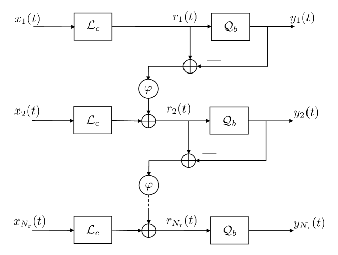
Quantization noise from each antenna is fed back along with the input of the next antenna to realize the architecture in space. Due to the presence of the feedback, the quantization noise in a spatial ADC may become unbounded, overloading the output [22, 12]. To prevent overloading, the input signal, , is clipped using with clipping level as
where the operator is defined as and . The clipped signal is then quantized using a 1-bit quantizer with quantization voltage level as
Let denote the input to channel of the ADC at time . Then the corresponding output is given by
| (1) |
where is the quantization error. The quantization error at channel is phase shifted by and added to the input of channel as
| (2) |
where with being the steering angle and being the inter-element spacing in the array in wavelengths. Since there is no feedback to the first channel, . From (1) and (2), we have the recursion
| (3) |
We are interested in estimating parameters underlying the input signal from the output of the 1-bit spatial ADC . This is a challenging problem because of the cascade of two non-linearities in (II). Moreover, the information loss introduced by the 1-bit spatial ADC is mainly determined by the clipping level and the quantization level . For a given quantization level , we can prevent the system from overloading by choosing the clipping voltage as [12]
| (4) |
A small value of leads to severe loss in the input information due to clipping, which cannot be compensated later by any choice of the quantization level . Hence, it is necessary to choose a sufficiently large to avoid information loss due to clipping. In this work, we propose to choose such that for appropriately selected constants . See Section V-C for more details on the selection of . With such a choice of , the output of the clipper can be approximated as . Then the 1-bit spatial recursion in (II) simplifies to
| (5) |
where the lower triangular matrices and are defined as
with being the identity matrix. The architecture of the first-order 1-bit spatial ADC is shown in Fig. 1.
III Quantization noise modeling
Quantization is a non-linear and irreversible operation that makes its statistical analysis complicated. To simplify the analysis of a quantizer, the usual approach is to linearize the quantizer and account for the error due to linearization through additive noise, which is often assumed to be uniformly distributed and uncorrelated with the input of the quantizer [23, 22, 10, 11, 12]. However, this assumption is reasonable only for a multi-level quantizer with many levels and when the input has a sufficiently large dynamic range. This classical approach of modeling the approximation error due to linearization as additive uniform noise is not suitable for 1-bit quantizers. Therefore, in what follows, we develop a noise model for 1-bit spatial ADCs.
To begin with, we first express the input-output relation of a spatial ADC in terms of the function by drawing inspiration from [22], where a similar expression for the deterministic error in a temporal 1-bit quantizer was developed. Next, we propose to linearize the function by interpreting it as a multi-level quantizer to compute the second-order statistics of the quantization noise that is useful for decorrelating observations when solving parametric estimation and detection problems involving 1-bit spatial ADCs.
The error in (1) due to 1-bit spatial quantization admits a closed-form expression as given in the next Lemma.
Lemma 1.
For a 1-bit spatial ADC with , the quantization error as a function of the input is given by
| (6a) | |||
| (6b) | |||
for . Here, is the fractional part function.
The above expressions are derived in the appendix. Let us collect the output of all the channels of the 1-bit spatial ADC in a vector and rewrite (5) as
| (7) |
From Lemma 1, we have
| (8) |
where with , is the length- column vector with all ones, and the fractional part function is applied elementwise. Using the fact that , and from (7), the deterministic relation between the input and output of a 1-bit spatial ADC is given by
| (9) |
where we have transformed the non-linearity due to the 1-bit quantization to the non-linear function.
Now we leverage the fact that the input-output relation of a function is similar to that of a multi-level quantizer with a step size of one. For the spatial ADC channels (corresponding to antenna elements) with larger indices that are away from the st channel, the dynamic range of the real and imaginary parts of is large when compared to . This means that for antenna elements with indices away from the st element, the function acts like a multi-level quantizer with an input having a large dynamic range. Therefore, it is now reasonable to model the approximation error due to the linearization of the function as additive noise, , which is uniformly distributed and uncorrelated with the input for channels having larger indices, i.e., we have
with the real and imaginary parts of . Substituting in (9) yields
| (10) |
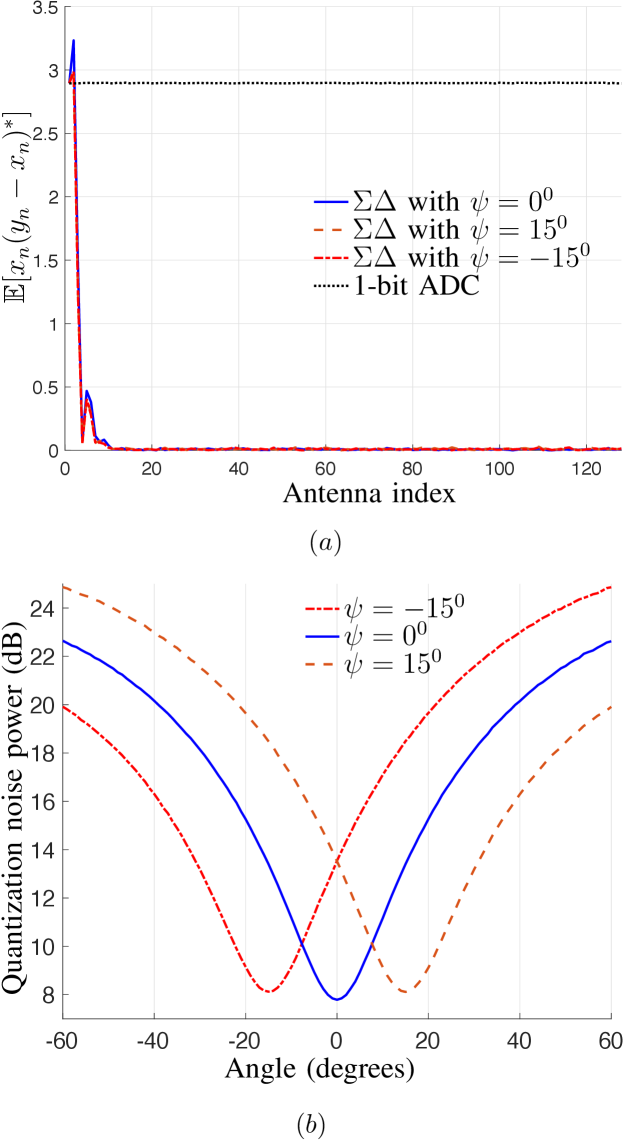
where , which is an affine transformation of , is also uniformly distributed and is uncorrelated with the input for larger channel (or antenna) indices . In massive MIMO systems with large number of antennas, there are many antennas for which and are uncorrelated. The correlation of with , i.e., for an antenna array having elements with an inter-element spacing of one eighth the signal wavelength is illustrated in Fig. † ‣ 2(a).
The covariance matrix of the noise vector in (10) is given by . When , the matrix with ones on the main diagonal, on the first sub-diagonal, and zeros elsewhere, is a spatial high-pass filter, which shapes the quantization noise to higher spatial frequencies. We illustrate the angular power spectrum of the quantization noise, i.e., , for different values of the steering angle in Fig. † ‣ 2(b), where is the steering vector of the uniform linear array (ULA) having elements at the BS with an inter-element spacing wavelengths. We can see that the quantization noise is very small for the directions around the steering angle.
Before we end this section, we make the following two remarks. Although in the development of the noise model, the spatial ADC is steered to the array broadside with for ease of exposition, introducing a phase shift in the feedback does not alter the uncorrelatedness between the input and the quantization noise as can be seen in Fig. † ‣ 2(a). Next, for the function in (9) to behave as a multi-level quantizer, the quantization voltage level plays an important role. When is very large, the dynamic range of the real and imaginary parts of the argument of the function, i.e., , can be very small for which the uniform noise or uncorrelated noise assumption might fail. Hence, carefully selecting (as discussed in Section V-C) becomes crucial.
Next, we use the developed spatial signal and noise models to estimate MIMO channels with angular models.
IV Angular channel model
In this paper, we consider the two commonly encountered SU-MIMO and MU-MIMO settings in MIMO communications. In the SU-MIMO setting, a single UE with antennas communicates with a multi-antenna BS, whereas in the MU-MIMO setting, single antenna UEs communicate with a multi-antenna BS. In both these settings, the BS has a ULA with antennas and it receives and processes uplink training pilots.
Let us collect the uplink training pilots in , where is the pilot length. Without loss of generality, let us assume that the columns of the pilot matrix have unit norm. Let denote the total transmit power at the UE and denote the MIMO channel matrix. The signal received at the BS prior to quantization, denoted as , can be expressed as
| (11) |
where is also the uplink SNR of the system and is the additive white Gaussian receiver noise matrix with entries . The received signal is then quantized using an -channel 1-bit spatial ADC to obtain , which is given by
Next, we parameterize by assuming a narrowband spatially sparse model for MU-MIMO and SU-MIMO systems.
IV-A SU-MIMO channel model
Suppose there are scatterers that result in paths between the UE and BS. Let us denote the AoDs of the paths from the UE by , the AoAs of the paths at the BS by , and the complex path gains by . The MIMO channel matrix is then expressed in terms of these parameters as
| (12) |
where is the array manifold of the ULA at the BS and is the array manifold at the UE. The columns of contain the array response vector of the critically spaced ULA at the UE with elements, and is given by . Similarly, the columns of contain the array response vector of the oversampled ULA at the BS with an inter-element spacing wavelengths, and is given by .
IV-B MU-MIMO channel model
Suppose that there are single antenna users. The SIMO channel between the th UE and the BS with paths is given by
| (13) |
where denotes the array manifold at the BS, collects AoAs of paths from th UE at the BS, and denotes the corresponding complex path gains. Then the overall channel matrix for the MU-MIMO system is given by
V SU-MIMO channel estimation
In this section, we present the proposed algorithm for channel estimation with angular models in SU-MIMO systems having 1-bit spatial ADCs at the BS. Specifically, we propose a two-step algorithm to estimate the channel parameters from uplink pilots. In the first step, we estimate the AoAs (i.e., ) and the path gains (i.e., ) using precoded uplink pilots, which excite all the angles uniformly. Next, in the second step, to estimate the AoDs, i.e., , we select precoders from a codebook using a recursive bisection procedure that leverages 1-bit feedback between the BS and UE to reduce the number of channel uses and thus the channel estimation overhead.
As we discuss later, it is crucial to carefully select the clipping voltage levels to benefit from the advantages of the 1-bit spatial ADCs. The proposed two-step channel estimation procedure is developed keeping in mind the dependence of the unknown parameters on voltage level selection.
V-A Step 1: AoA and path gain estimation
V-A1 AoA estimation
To estimate the AoAs at the BS, the UE transmits precoded pilot symbols for , where is the precoder with so that the total transmit power is . As we do not yet know the AoDs, instead of selecting to focus energy in specific directions, we select it such that all the departure angles are excited uniformly as
| (14) |
where denotes the set of candidate AoDs. An obvious choice of that satisfies (14) is
| (15) |
This means that we turn off all the antennas at the UE except the first one to perform an omnidirectional transmission.
From (10), the symbols received at the BS in Step 1 can be compactly expressed as
| (16) |
where is the transmitted pilot matrix and the effective noise matrix is defined as is the sum of the receiver noise and the quantization noise . The matrix has all one entries. Thus, the precoder in (15) makes independent of the AoDs.
The AoAs can now be estimated from using standard direction-finding techniques like Bartlett beamforming, minimum variance distortionless response (MVDR) beamforming [24], sparse recovery, or using a maximum likelihood based estimator. Since a massive MIMO BS typically has a large number (of the order of hundreds) of antennas, we may use a computationally less intensive method, such as the Bartlett beamforming for AoA estimation. Specifically, the AoA estimates, denoted by , are the locations of the local maxima of the Bartlett spatial spectrum
| (17) |
where is the sample covariance matrix.
V-A2 Path gain estimation
Next, to estimate the path gains, we form the estimated array manifold at the BS as and approximate (16) as
| (18) |
Recall from the quantization noise modeling in Section III that the covariance matrix of the quantization noise is given by and that the quantization noise is uncorrelated with the input. Thus the covariance matrix of the effective noise term in (16) is
| (19) |
We now prewhiten the observations to obtain
where is the prewhitening matrix, which can be obtained using an eigenvalue decomposition of and is the whitened noise term. Using the property that , we have with and as the BS usually has large number of antennas and the mmWave MIMO channel is sparse in the angular domain. The path gains can then be estimated using least squares as
| (20) |
V-B Step 2: AoD estimation
Now what remains is to estimate the AoDs. To do so, we propose a recursive bisection procedure, which divides the spatial sector into two subsectors at each stage and measures the power of the signal received in the direction corresponding to the estimated AoA. The method selects the subsector with the largest received power as the new sector to be used in the next bisection stage. This procedure is continued till the desired subsector resolution is obtained and is repeated for each of the estimated AoAs corresponding to paths.
Let us denote the precoder that we use in Step 2 by with , as before. Let us also define the inner product between and as , where we have and when , the upper bound is achieved with equality. Therefore, by choosing a precoder that yields the maximum , we can indirectly refine the AoD sector of the th path to compute the AoD.
Suppose the UE transmits precoded symbols , where the subscript “2” denotes Step 2 of the algorithm. Using the combiner , the component of the received uplink pilot arriving along the th path at the BS can be expressed as
| (21) |
Since we have a large array at the BS and assuming that the AoAs are sufficiently separated, we can approximate for . Using this approximation and multiplying both sides of (21) with , we have
| (22) |
which allows us to compute the energy of the received symbols arriving from the th path as
| (23) |
In practice, we compute using the estimate from Step 1 to form the combiner as .
We can estimate the AoDs by finding precoders, , that maximize for each path , where recall that the structure of the precoder vector is constrained to . Here, we assume that the number of paths, , is known. Performing this maximization by exhaustively searching over all the departure angles in a predefined grid results in excessive training overhead. Therefore, we present a recursive bisection procedure, where for each path , we start with a wide beam and progressively refine it to maximize .
V-B1 Design of the precoder codebook
Before we describe the proposed recursive biscection procedure, we first provide the design of a codebook that contains precoders required for each stage of the procedure. Let us discretize the departure angular domain into grid points by uniformly sampling the direction cosine space so that for . Let us define the index set as
for with . Next, we the partition the set into partitions for the th stage of the recursive procedure with a total number of stages. In other words, at Stage , we have spatial sectors with the th sector formed from angles and in the last stage, i.e., at Stage , we have sectors with angular grid points in . For example, in the first stage, we have two spatial sectors and .
Let denote the th precoder for the th stage. The precoders are designed to focus on a desired angular sector as
| (24) |
for and . Defining the dictionary matrix with , and the precoder matrix , we can compactly express (24) as the linear system
| (25) |
where the desired beampattern matrix with being the indicator vector with entries equal to one at locations indexed by the set . Then the precoders for the th stage can be computed using least squares as
| (26) |
To obtain unit-norm precoding vectors, we normalize each column of to unity. We repeat this procedure for to compute precoders for all the stages. This completes the design of the precoder codebook.
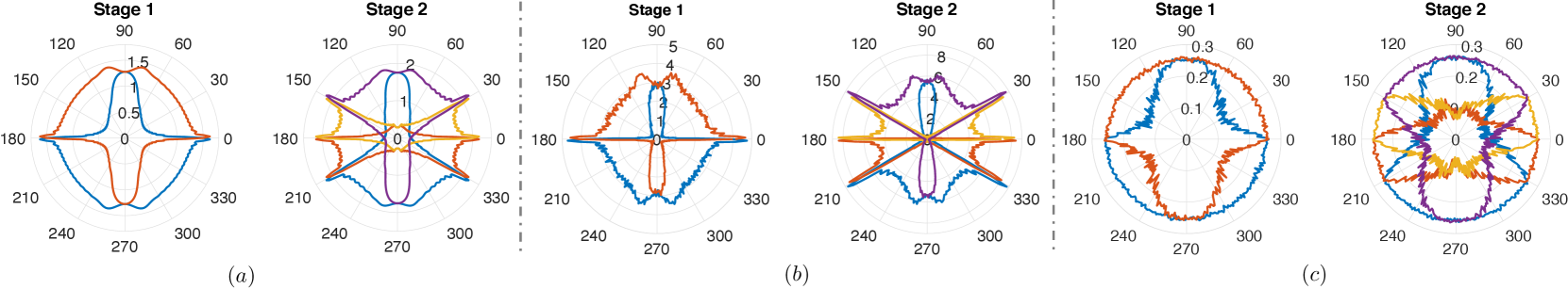
In Fig. 3(a), we show the beampattern for corresponding to Stage 1 with and Stage 2 with of the codebook. In Figs. 3(b) and 3(c), we show the beampatterns corresponding to the first two stages as seen by the BS without any quantizer, i.e., and by the BS with 1-bit ADC, i.e., , respectively, where as in (11), as in (10), and we vary and as before. Here, we use , , , and SNR of 10 dB. We see that the received beampattern in Fig. 3(c) is significantly distorted as the 1-bit ADC is not steered to the , i.e., , and more importantly, because the quantization voltage level is set to an arbitrary level. While we can steer the 1-bit ADC based on the AoA estimate from Step 1 as , we emphasize that a procedure to select an appropriate voltage level is crucial. Before describing the procedure to select , we next present the recursive bisection procedure to estimate the AoDs.
V-B2 Recursive bisection procedure
We estimate the AoDs of the th path by maximizing in (23) by recursively bisecting the spatial sector and selecting a subsector that yields the highest received energy. The BS informs via a 1-bit error-free feedback link the selected subsector to the UE, which further bisects the selected subsector to transmit pilots for the next stage. The procedure is continued for stages, where at the last stage, we select one of the angular grid points in as the estimated AoD of the th path. We repeat this procedure for all the paths.
To estimate the AoD of the th path, we proceed as follows. Recall from (24) that has a unit response in the sector formed by departure angles . In the first stage, the UE transmits pilots using precoders and . The BS then computes the energy of the received symbols using (23) and selects the subsector (or the precoder) that yeilds . If , the BS sends a feedback of 0 to the UE through an error-free 1-bit feedback link indicating that the sector is selected. Similarly, it sends a 1 indicating that the sector is selected. In the second stage, the UE then bisects the selected subsector and transmits pilots using the precoders (respectively, ) if the received feedback from the BS is 0 (respectively, 1). More generally, at Stage s, suppose the UE transmits pilots using precoders and . The BS transmits a 1 to the UE, which then selects the precoders corresponding to a narrower subsector for the next stage. We continue this procedure for stages, where the partition selected in the final stage corresponds to the index of the estimated AoD. The same procedure is repeated for all the paths.
V-C Selection of clipping and quantization voltage levels
In Fig. 3(c), we have seen that the choice of and play a crucial role in determining the channel estimation and beamforming performance of MIMO systems with 1-bit spatial ADCs. As discussed in Section II, we choose the clipping level based on the standard deviation of input that allows us to place a bound on the clipping error using the Chebyshev inequality for constants . Therefore, the choice of depends on the statistics of the unquantized signal received at the BS, leading to different choices of voltage levels for Step 1 and Step 2 of the proposed channel estimation algorithm.
V-C1 For estimating AoAs and path gains in Step 1
From (16) and (10), the unquantized signal received at the th antenna of the BS in Step 1 of the proposed channel estimation technique is
where and follow a complex Gaussian distribution with zero mean and unit variance. Since the complex path gains and the additive noise are mutually independent, follows a complex Gaussian distribution with zero mean and variance . In other words, and . Let us recall that the probability that a Gaussian random variable takes values away from the mean by more than thrice the standard deviation is less than . Hence, to ensure
in Step 1, we choose the clipping voltage level
| (27) |
The clipping voltage level for the imaginary part is computed similarly. The quantization voltage level is then selected using the overload condition (4).
V-C2 For estimating AoDs in Step 2
In the second step, from (21) and (10), the unquantized signal received at the th antenna of the BS related to the uplink pilot transmission with the precoder is
where follows a complex Gaussian distribution with zero mean and variance . Since is bounded from above by , the worst-case variance of is . Therefore, we choose the clipping level as
| (28) |
in Step 2, to ensure that the worst-case clipping probability of , is less than 1.
Since the clipping voltage level that we select in Step 1 is different from Step 2, a joint estimator (e.g., sparse recovery based method as in [3]) to jointly estimate the channel parameters is not straightforward when dealing with observations from 1-bit spatial ADCs.
V-D Computations and number of pilot transmissions
In Step 1, we transmit pilots. In Step 2, we transmit each beam times with 2 beams in each stage. Since there are stages, and paths, the total pilot transmission overhead in the second stage is .
For a search grid of size , computing the Bartlett beamforming spectrum in (17) costs about order flops. The least squares estimator to compute the path gains incurs about order flops. In Step 2, for each beam and path, we compute the received power, which costs about order flops. In contrast, a scheme that exhaustively searches over all possible AoA and AoD combinations with pilot transmissions incurs a computational complexity of about order flops, which is higher than flops incurred by the proposed method as typically . The computational complexity of the proposed channel estimation algorithm scales linearly with the number of receive antennas and log-linearly with the search grid size, thus making it well-suited for massive MIMO systems.
VI MU-MIMO channel estimation
In this section, we specialize the proposed channel estimation algorithm to the MU-MIMO setting with the angular channel model described in Section IV-B. We estimate the channel by estimating the AoAs and the path gains using Step 1 of the algorithm developed in the previous section. Since we assume that the UEs have a single antenna in the MU-MIMO setup, there is no AoD estimation step.
Let denote the orthogonal pilot matrix transmitted at time instance from the UEs such that . From (11) and (10), the received signal at the BS with 1-bit spatial ADC is
where is the total number of channel uses, is the sum of additive white Gaussian noise and quantization noise, as defined before. Using the known pilots, we preprocess the received signal to separate the signal components from the UEs to obtain where the th column of , denoted by , is related to the SIMO channel between the th UE and the BS at time instance , and is given by [cf. (13)]
Here, denotes the th column of . Suppose and . Then we have which readily resembles the signal model in (16). Therefore, we can use Step 1 of the SU-MIMO channel estimation algorithm developed in the previous section to estimate the channel parameters for each user. Also, we choose the same voltage level as the one used in Step 1 of SU-MIMO channel estimation.
VII Numerical simulations
In this section, we present results from a number of numerical simulations to demonstrate the efficacy of the developed quantization noise model, voltage level selection, and channel estimation algorithms in mmWave MIMO systems with 1-bit spatial ADCs. We compare different algorithms in terms of normalized mean square error (NMSE) and angle estimation error. We define NMSE of a path gain estimate and a channel estimate as
and
respectively. Let denote the AoA search grid of size used in (17). Let us denote the index set of AoAs corresponding to the angles in as
Let us also denote the index set of AoDs corresponding to the angles in AoD grid of size as
We then define the AoA and AoD estimation errors as
where and are the estimated AoAs and AoDs, respectively.
VII-A The SU-MIMO setting
We consider a SU-MIMO setup with the UE having antennas, the BS having antennas that are spaced wavelengths apart. For Bartlett beamforming, we use the search grid with points. The AoD grid is obtained by uniformly sampling the direction cosine space in the interval to with points as described in Section V-B1.
VII-A1 Angle steering and voltage level selection
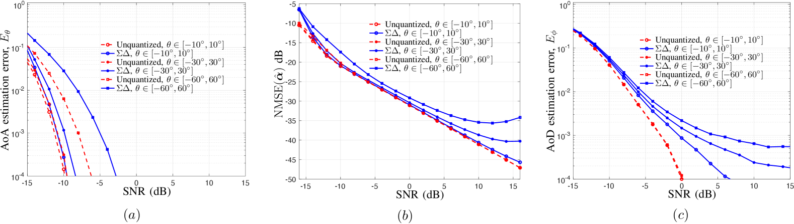
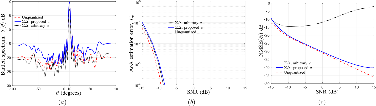
We first begin with a discussion on the estimation performance of the channel parameters in Step 1 and in Step 2 of the proposed channel estimator for a single path channel with . This allows us to discuss the impact of voltage level selection and angle steering on the estimators. The AoA is drawn uniformly at random from the sector for . The AoD is drawn randomly from the sector . The path gain is assumed to be unit modulus. We use and . Unless otherwise mentioned, we use independent channel realizations to compute NMSE and angle errors. In this subsection, we compare the estimation performance of the proposed technique with 1-bit spatial ADC, referred to as “”, with an equivalent channel estimation method applied on unquantized data (wherein the BS is assumed to have a very high-resolution ADC). We label it as “Unquantized” in the plots. Since estimates from “Unquantized” will be better than the same scheme applied on quantized data for a comparable number of snapshots, we use this as a baseline to illustrate the loss due to 1-bit ADC.
We illustrate the channel estimation performance for different SNRs in terms of in Fig. 4(a), in Fig. 4(b) and in Fig. 4(c). Here, “Unquantized, ” and “” indicate that the AoA is drawn uniformly at random from the sector in each channel realization. We can see that “” performs similar to that of “Unquantized” for the path with AoA arriving close to the array broadside, whereas the gap between “Unquantized” and “” increases for the path arriving with angles away from the array broadside. This is mainly due to the quantization noise shaping at higher spatial frequencies. Performance degradation at higher SNRs is inevitable due to the larger choice of at high SNRs, which results in higher quantization noise [cf. (19)].
Next, in Fig. 5(a), Fig. 5(b), and Fig. 5(c), respectively, we illustrate the impact of clipping voltage level selection on , , and by comparing the proposed clipping voltage level from Section V-C1 with a fixed, SNR independent arbitrary clipping voltage level . While we observe that the Bartlett beampatterns as well as the AoA estimation errors are not sensitive to the choice of clipping voltage levels, we, however, can observe from Fig. 5(c) that not selecting a correct clipping voltage level leads to severe performance degradation in path gain estimation. In other words, Fig. 5(c) demonstrates that a blind application of least squares without an appropriate selection of the clipping voltage level does not result in satisfactory performance.
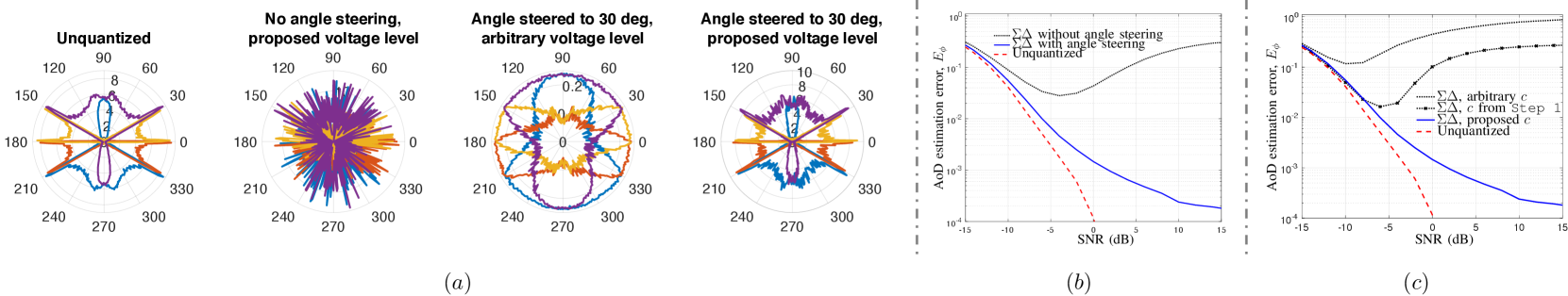
Recall in Fig. 3(c), we discussed the impact of clipping voltage level selection and angle steering on the beampatterns in Step 2 as observed at the 1-bit spatial ADC. We now extend that discussion in Fig. 6(a), where we focus on the second stage of the proposed codebook as observed at the receiver of an unquantized system and compare it to the beampattern as seen at the receiver with a 1-bit spatial ADC. We consider a scenario where the path arrives at the BS with an AoA of and an SNR of dB. We observe that the beampatterns are severely distorted whenever the steering angle, voltage level, or both are incorrectly selected. Nevertheless, with a careful selection of voltage levels and steering angle, the beampatterns at the receiver with a 1-bit spatial ADC are comparable to that of the unquantized system.
In Fig. 6(b) and Fig. 6(c), we demonstrate, respectively, the impact of angle steering and clipping voltage level selection on AoD estimation, where the AoA is drawn uniformly at random from the sector in each channel realization to compute . We can observe that failing to exploit angle steering leads to serious loss in performance. While clipping voltage selection was not crucial for AoA estimation, we observe that fixing the voltage level to an arbitrary value, such as , or varying it in an inappropriate manner, e.g., using the clipping voltage level designed for Step 1 in Step 2 (indicated as “, from Step1”), do not provide satisfactory AoD estimation performance. In other words, a direct application of existing hierarchical codebook-based channel estimation methods, e.g., [3] without a careful selection of clipping voltage levels and phase shifts in the feedback loop will not provide reasonable performance for MIMO systems with 1-bit spatial ADCs.
VII-A2 Multipath channel
We now consider a multipath SU-MIMO channel with , which are typical at mmWave frequencies. We assume that the complex path gains follow a truncated Gaussian distribution with for . To ensure that all the paths are sufficiently strong, we choose . The AoDs are drawn uniformly at random from the sector with a minimum spacing of in the direction cosine space and the AoAs are drawn uniformly at random from the sector with a minimum spacing of , where . We choose and . Recall that the proposed method with 1-bit spatial ADC, referred to as “”, requires reception of pilots in Step 1 and pilots in Step 2, where the reception at each step is with a different clipping voltage level. Hence, designing a scheme that utilizes all the available measurements for channel estimation with 1-bit spatial ADCs is not straightforward.
We compare the performance of the proposed method with amplitude retrieval based one-bit SU-MIMO channel estimation algorithm [19], referred to as “AR” in the plots. In “AR”, after the amplitudes are recovered from one-bit measurements, standard channel estimation algorithm can be used. Since “AR” does not involve any clipping voltage selection, here, we use all the measurements to perform amplitude recovery as in [19], AoA and path gain estimation using Step 1 and AoD estimation using Step 2 as described in Section V. In addition to “Unquantized”, which serves as a benchmark for “” as it uses pilots in Step 1 and pilots in Step 2, we also report the performance of an unquantized system, labelled as “Unquantized full data”, that uses all the pilots in both Step 1 and Step 2. Thus, the total number of pilot transmissions in all the methods that we compare with are the same. We have observed the runtime of the “AR” algorithm is significantly higher than the proposed method. Due to this reason, we use independent Monte-Carlo (MC) experiments to compute the NMSE of “AR”, whereas MC experiments are used to obtain plots for “Unquantized,” “Unquantized full data,” and “” methods. NMSE of “AR” is, in general, much higher than that of the other methods, which suggests that a fewer number of MC runs is sufficient to obtain curves of comparable precision.
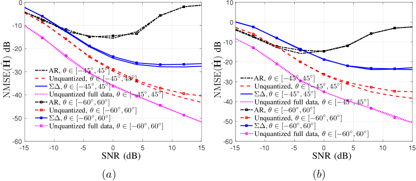
In Fig. 7, we show the channel estimation NMSE, where or indicate the sector from which the AoAs are drawn in each channel realization. We can observe that the performance of “” is comparable to that of “Unquantized” and is better than that of “AR” except at very low SNRs. At extremely low SNRs, we observe that the performance of “AR” is slightly better than that of “Unquantized” and “” as the effective number of snapshots available to estimate the channel parameters is larger for “AR”. At high SNRs, on the other hand, higher quantization noise in 1-bit systems leads to a deteriorated performance of “AR”. Similarly, at high SNRs and for angles away from broadside, there is an inevitable gap between the NMSE of “” and “Unquantized” due to the increase in the quantization noise. Furthermore, the NMSE of channel estimation for is slightly larger than that of due to the larger number of parameters to be estimated in the latter case. As expected, the benchmark scheme “Unquantized full data” has the lowest NMSE due to the absence of quantization and efficient use of all available snapshots to carry out channel estimation. In essence, the proposed method achieves performance comparable to that of “Unquantized” and significantly better than that of “AR” for most of the SNRs, making it an attractive choice for massive MIMO systems.
VII-B The MU-MIMO setting
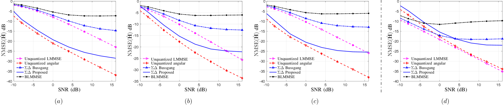
For the MU-MIMO setting, we consider users and a BS having antennas that are wavelengths apart. We use for , , and use independent channel realizations for computing NMSE. For each path, the AoAs are drawn uniformly at random from the sector with a minimum spacing of . We compare the channel estimation performance of the proposed method, referred to as “ proposed” with the following state-of-the-art techniques in MU-MIMO channel estimation: (A) Bussgang decomposition followed by computing LMMSE MU-MIMO channel estimation for 1-bit MIMO systems [6], referred to as “BLMMSE”, (B) MU-MIMO channel estimation with 1-bit spatial ADC based on the Bussgang decomposition [14], labelled as “ Bussgang”, (C) an LMMSE MU-MIMO channel estimator that uses unquantized data, referred to as “Unquantized LMMSE”, and (D) the proposed channel estimation algorithm from Section IV-B applied to unquantized data, referred to as “Unquantized angular”. “Unquantized angular” serves as the benchmark scheme for “ proposed” and illustrates the loss due 1-bit spatial quantization. We reemphasize that “Unquantized LMMSE”, “BLMMSE”, and “ Bussgang” require the channel correlation information to perform the Bussgang decomposition and for subsequent channel estimation, and that this amounts to knowing the angles that parameterize the angular channel model. However, for the sake of comparison, we generate an approximate channel correlation by assuming that each UE has paths, each separated by 1 degree in the range of with [cf. (13)].
The NMSE performance of different methods for , and are presented in Fig. 8(a), Fig. 8(b), and Fig. 8(c), respectively. It can be observed that the proposed scheme performs better in terms of NMSE than existing methods, namely, “BLMMSE” and “ Bussgang”. At low-to-moderate SNRs, the performance of “ Proposed” is comparable to that of “Unquantized angular”. This corroborates the developed theory that 1-bit spatial ADCs have higher effective resolution, which can be leveraged for parametric estimation. At higher SNRs, the NMSE performance reduces for both “ Bussgang” and “ Proposed” due to the inevitable increase in quantization noise that is bound to occur at high SNRs. Nonetheless, even at high SNRs, the proposed method outperforms “ Bussgang” by a margin of about (respectively, ) for (respectively, ).
As expected, the performance of the parametric channel estimation techniques (i.e., “Unquantized angular” and “ Proposed”) is better than their non-parametric counterparts (i.e., “Unquantized LMMSE” and “ Bussgang”) as the parametric techniques exploit the structure in the angular channel model. As expected, the channel estimation performance of “ Proposed” and “Unquantized angular” is better in Fig. 8(a) with as compared to the multipath scenario in Fig. 8(b). Furthermore, in Fig. 8(a), we can see that “ Proposed” is about better when compared to the state-of-the-art method “ Bussgang”. Also, when is doubled from in Fig. 8(b) to in Fig. 8(c), due to the improved resolution and quantization noise shaping of the larger antenna array in the latter, we see that the proposed technique significantly outperforms existing techniques.
In Fig. 8(d), we compare the performance of the proposed channel estimator when the true channel correlation is used to compute the Bussgang decomposition. In this setting, though not realizable in practice, “Unquantized LMMSE” is the optimal channel estimator. We can see that “Unquantized angular”, which is the proposed technique that works with unquantized data performs similar to that of the optimal estimator at low-to-moderate SNRs. Also, we can see that the performance of our method is comparable (in terms of channel estimation NMSE) to “ Bussgang” at moderate-to-high SNRs.
VIII Conclusions
In this paper, we have presented an algorithm for channel estimation with angular models in massive MIMO systems employing 1-bit spatial ADC. We have developed a quantization noise model for 1-bit spatial ADCs that is useful, in general, for large array processing applications. Although computing the complete quantization noise probability density function is difficult, the developed noise model allows us to compute its second-order statistics that can be used to prewhiten data when solving parametric estimation problems. When the quantization voltage levels and phase shifts in the feedback loop are carefully selected, the effective resolution of 1-bit spatial ADCs can be improved and hence are comparable to unquantized systems in most operating regimes of interest. We have developed a two-step channel estimation procedure to estimate the AoAs, AoDs, and path gains that characterize the MIMO channel. The proposed algorithm allows us to select the phase shifts and quantization voltage levels, which depend on the unknown channel parameters. Through numerical simulations, we have demonstrated that with the proposed channel estimation algorithm, MIMO systems with 1-bit spatial ADCs perform significantly better than MIMO systems with regular 1-bit quantization and are often on par with that of unquantized MIMO systems for low-to-moderate SNRs. [Proof of Lemma 1] The expressions in (6) are obtained by adapting the derivation in [22] to 1-bit spatial ADCs and are derived here for self containment.
From (1) and (2) with , we have the recursion
| (29) |
Let us define the normalized quantization error as
| (30) |
where and as the quantization error is bounded when the voltage levels are chosen as in (4).
Using (1), we can express and in terms of the input and output of the quantizer as
| (31) |
with
When , or equivalently, when , we have . This allows us to constrain (31) as
Thus, as the fractional part function for . Similarly, when , or equivalently, when , we have ,
and
| (32) |
where the lower and upper bounds are due to the fact that and due to clipping . For , we have Therefore, when , from (32), we again have
| (33) |
Recursively substituting for , , and so on in (33), and using the fact that , we obtain
Using the above expression in (30) yields
Using the fact that , , the above expression can be equivalently expressed as (6a). The expression for the imaginary part in (6b) can be derived along the same lines.
References
- [1] R. S. P. Sankar and S. P. Chepuri, “Millimeter wave MIMO channel estimation with 1-bit spatial sigma-delta analog-to-digital converters,” in Proc. of the IEEE International Conference on Acoustics, Speech, and Signal Processing (ICASSP), Toronto, Canada, Jun. 2021.
- [2] T. S. Rappaport, S. Sun, R. Mayzus, H. Zhao, Y. Azar, K. Wang, G. N. Wong, J. K. Schulz, M. Samimi, and F. Gutierrez, “Millimeter wave mobile communications for 5G cellular: It will work!” IEEE Access, vol. 1, pp. 335–349, May 2013.
- [3] A. Alkhateeb, O. E. Ayach, G. Leus, and R. W. Heath, “Channel estimation and hybrid precoding for millimeter wave cellular systems,” IEEE J. Sel. Topics Signal Process., vol. 8, no. 5, pp. 831–846, Oct. 2014.
- [4] A. Ghosh, T. A. Thomas, M. C. Cudak, R. Ratasuk, P. Moorut, F. W. Vook, T. S. Rappaport, G. R. MacCartney, S. Sun, and S. Nie, “Millimeter-wave enhanced local area systems: A high-data-rate approach for future wireless networks,” IEEE J. Sel. Areas Commun., vol. 32, no. 6, pp. 1152–1163, June 2014.
- [5] J. Mo and R. W. Heath, “Capacity analysis of one-bit quantized MIMO systems with transmitter channel state information,” IEEE Trans. Signal Process., vol. 63, no. 20, pp. 5498–5512, Jul. 2015.
- [6] Y. Li, C. Tao, G. Seco-Granados, A. Mezghani, A. L. Swindlehurst, and L. Liu, “Channel estimation and performance analysis of one-bit massive MIMO systems,” IEEE Trans. Signal Process., vol. 65, no. 15, pp. 4075–4089, Aug. 2017.
- [7] K. Roth, H. Pirzadeh, A. L. Swindlehurst, and J. A. Nossek, “A comparison of hybrid beamforming and digital beamforming with low-resolution ADCs for multiple users and imperfect CSI,” IEEE J. Sel. Topics Signal Process., vol. 12, no. 3, pp. 484–498, Mar 2018.
- [8] P. M. Aziz, H. V. Sorensen, and J. Van Der Spiegel, “An overview of sigma-delta converters: How a 1-bit ADC achieves more than 16-bit resolution,” IEEE Signal Process. Mag., vol. 13, no. 1, pp. 61–84, Jan. 1996.
- [9] R. M. Corey and A. C. Singer, “Spatial sigma-delta signal acquisition for wideband beamforming arrays,” in Proc. Int. ITG Workshop Smart Antennas, Munich, Germany, Mar. 2016.
- [10] D. Barać and E. Lindqvist, “Spatial sigma-delta modulation in a massive MIMO cellular system,” Master’s thesis, Chalmers University of Technology, Sweden, June 2016.
- [11] V. Venkateswaran and A.-J. van der Veen, “Multichannel ADCs with integrated feedback beamformers to cancel interfering communication signals,” IEEE Trans. Signal Process., vol. 59, no. 5, pp. 2211–2222, May 2011.
- [12] M. Shao, W. Ma, Q. Li, and A. L. Swindlehurst, “One-bit sigma-delta MIMO precoding,” IEEE J. Sel. Topics Signal Process., vol. 13, no. 5, pp. 1046–1061, Sept. 2019.
- [13] S. Rao, A. L. Swindlehurst, and H. Pirzadeh, “Massive MIMO channel estimation with 1-bit spatial sigma-delta ADCs,” in Proc. of the IEEE Int. Conf. on Acoustics, Speech and Signal Process. (ICASSP), Brighton, UK, May 2019.
- [14] S. Rao, G. Seco-Granados, H. Pirzadeh, J. A. Nossek, and A. L. Swindlehurst, “Massive MIMO channel estimation with low-resolution spatial sigma-delta ADCs,” IEEE Access, vol. 9, pp. 109 320–109 334, Jul. 2021.
- [15] H. Pirzadeh, G. Seco-Granados, S. Rao, and A. L. Swindlehurst, “Spectral efficiency of one-bit sigma-delta massive MIMO systems,” IEEE J. Sel. Areas Commun., vol. 38, no. 9, pp. 2215–2226, Sept. 2020.
- [16] J. J. Bussgang, “Crosscorrelation functions of amplitude-distorted Gaussian signals,” Technical report, Research Laboratory of Electronics, Massachusetts Institute of Technology, Mar. 1952. [Online]. Available: http://hdl.handle.net/1721.1/4847
- [17] Ö. T. Demir and E. Björnson, “The Bussgang decomposition of non-linear systems: Basic theory and MIMO extensions,” arXiv preprint arXiv:2005.01597, May 2020.
- [18] S. Jacobsson, G. Durisi, M. Coldrey, U. Gustavsson, and C. Studer, “Throughput analysis of massive MIMO uplink with low-resolution ADCs,” IEEE Trans. Wireless Commun., vol. 16, no. 6, pp. 4038–4051, June 2017.
- [19] C. Qian, X. Fu, and N. D. Sidiropoulos, “Amplitude retrieval for channel estimation of MIMO systems with one-bit ADCs,” IEEE Signal Process. Lett., vol. 26, no. 11, pp. 1698–1702, Nov. 2019.
- [20] J. Mo, P. Schniter, N. G. Prelcic, and R. W. Heath, “Channel estimation in millimeter wave MIMO systems with one-bit quantization,” in Proc. of the Asilomar Conference on Signals, Systems and Computers, Pacific Grove, USA, Nov. 2014.
- [21] Y. Zhang, M. Alrabeiah, and A. Alkhateeb, “Deep learning for massive MIMO with 1-bit ADCs: When more antennas need fewer pilots,” IEEE Wireless Commun. Lett., vol. 9, no. 8, pp. 1273–1277, Apr. 2020.
- [22] R. M. Gray, W. Chou, and P. W. Wong, “Quantization noise in single-loop sigma-delta modulation with sinusoidal inputs,” IEEE Trans. Commun., vol. 37, no. 9, pp. 956–968, Sept. 1989.
- [23] R. M. Gray, “Oversampled sigma-delta modulation,” IEEE Trans. Commun., vol. 35, no. 5, pp. 481–489, May 1987.
- [24] H. L. Van Trees, Optimum Array Processing: Part IV of Detection, Estimation, and Modulation Theory. USA: John Wiley & Sons, Ltd, 2002.