Channel Mapping Based on Interleaved Learning with Complex-Domain MLP-Mixer

We consider a massive MIMO system, where a base station (BS) with $N_{\mathrm{t}}\gg 1$ antennas serves multiple single-antenna users. Also, the considered system adopts OFDM modulation with $N_{\mathrm{c}}$ subcarriers. The channel between one user and the BS is assumed to be composed of $P$ paths, which can be expressed as,

$${\bf{h}}\left(f\right)=\sum\limits_{p=1}^{P}{{\alpha_{p}}{e^{-j2\pi f{\tau_{p}}}}{\bf{a}}(\vec{p})},$$

(1)

where $f$ is the carrier frequency, ${\alpha_{p}}$ is the amplitude attenuation, ${\tau_{p}}$ is the propagation delay, and $\vec{p}$ is the three-dimensional unit vector of departure direction of the $p$-th path. Furthermore, $\mathbf{a}(\vec{p})$ is the array defined as,

$${\mathbf{a}(\vec{p})}={\left[{1,{e^{-j2\pi f{{\vec{d}_{1}}}\cdot\vec{p}/c}},\ldots,{e^{-j2\pi f{{\vec{d}_{{N_{\rm{t}}}-1}}}\cdot\vec{p}/c}}}\right]^{T}},$$

(2)

where $\left[{\vec{0},{{\vec{d}_{1}}},\ldots,{{\vec{d}_{{N_{\rm{t}}}-1}}}}\right]$ is the space vector array, ${{\vec{d}_{i}}}\leavevmode\nobreak\ (i=1,2,\ldots,{{N_{\rm{t}}}-1})$ represents the three-dimensional space vector between the $i$-antenna and the first antenna, and $c$ is the speed of light. The transmission distance shift between the $i$-th antenna and the first antenna on $p$-th path can be written as ${{\vec{d}_{i}}}\cdot\vec{p}$. If the antenna array form is a uniform linear array, ${{\vec{d}_{i}}}\cdot\vec{p}$ can be simplified as $id\cos{\theta_{p}}$, where ${\theta_{p}}$ is the angle of departure (AoD) of the $p$-th path and $d$ is the antenna space. This simplified case is equivalent to the channel model in the literature [5]. Further, the whole CSI matrix $\mathbf{H}\in{\mathbb{C}^{{N_{\mathrm{t}}}{\rm{\times}}{N_{\mathrm{c}}}}}$ between the user and the BS can be expressed as,

$\displaystyle\mathbf{H}=[\mathbf{h}({f_{1}}),\mathbf{h}(f_{2}),\cdots,\mathbf{h}({f_{N_{\mathrm{c}}}})],$

(3)

where ${f_{i}}={f_{0}}+\Delta{f_{i}},(i=1,2,\cdots,{N_{\rm{c}}})$, ${f_{i}}$ is the $i$-th subcarrier frequency, $f_{0}$ is the base frequency, and $\Delta{f_{i}}$ is the frequency shift between the $i$-th subcarrier and the base frequency.

As shown in the channel model, there are significant correlations within the CSI matrix, benefiting from the path-similarity of sub-channels. Further, channel mapping [2] aims at realizing such a task leveraging on this correlation: inputting sub-channels of some antennas and subcarriers to output the whole channel data, which can be written as,

$${\rm{g}}:{\bf{H}}[\Omega]\to{\bf{H}},$$

(4)

where $\Omega$ is the selected small subset in space and frequency, ${\bf{H}}[\Omega]$ is also written as ${\bf{H}}^{0}$.

The channel mapping task has many potential applications. For example, in high-dimensional channel estimation, it is possible only to estimate the CSI of several antennas and subcarriers and then obtain the whole channel by channel mapping to decrease the pilot overhead. Furthermore, in the high-dimensional CSI feedback, it is possible only to upload partial downlink CSI, and the BS can still reconstruct the whole downlink CSI based on channel mapping, forming a user-friendly CSI feedback scheme without the additional encoder. In Eq. (4), for the subset $\Omega$, a typical selection is the whole channel of several certain antennas and subcarriers, i.e.,

$\displaystyle\begin{array}[]{l}\Omega{\rm{=A}}\otimes{\rm{B}},\end{array}$

(6)

where $\rm{A}$ is the subset of the selected antennas, $\rm{B}$ is the subset of the selected subcarriers, and $\otimes$ represents that $\forall a\in{\rm{A\&b}}\in{\rm{B,}}\left({a,b}\right)\in\Omega$. Besides, the settings of A and B are often uniform distributions and as widely ranging as possible in space and frequency domains, respectively.

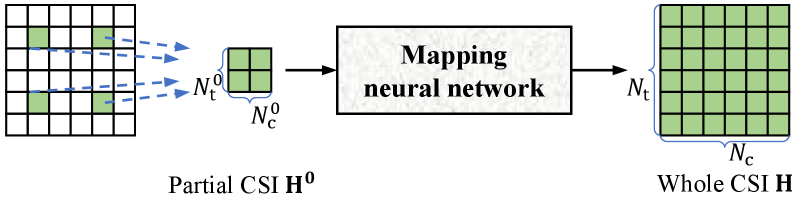
Since CSI is a complex coupling of multipath channel responses, the internal correlation in the CSI matrix is often implicit and, thus, is difficult to explore through traditional signal processing methods. Therefore, we use the DL technology with excellent implicit feature learning capabilities to realize efficient channel mapping. The overall DL-based channel mapping framework is shown in Fig. 1. This learning process mainly relies on the representation learning of channel data, i.e., representing implicit features from known channel information and then representing the whole channel based on the obtained features. For the mapping neural network, if some a priori design can be introduced according to the physical properties of the MIMO-OFDM channel, it will undoubtedly improve the representation learning and guide the network to learn more efficiently from the limited training data.

This subsection presents that there is an unique interlaced space and frequency characteristic in MIMO-OFDM channel. Specifically, according to the channel model in Section II-A, we can define the following function,

	$\displaystyle{q_{\bf{H}}}(\vec{d},\Delta f)=$
	$\displaystyle\sum\limits_{p=1}^{P}{{\alpha_{p}}{e^{-j2\pi{f_{0}}{\tau_{p}}}}{e^{-j\left({2\pi{f_{0}}\vec{d}\cdot\vec{p}/c+2\pi\Delta f{\tau_{p}}+2\pi\Delta f\vec{d}\cdot\vec{p}/c}\right)}}},$		(7)

where the parameters of ${q_{\bf{H}}}(\cdot)$, $\alpha_{p},f_{0},\tau_{p},{\vec{p}}$, are the shared large-scale features among all sub-channels. Therefore, ${q_{\bf{H}}}(\cdot)$ is independent of the specific antennas and subcarriers. Then, leveraging ${q_{\bf{H}}}(\cdot)$, the CSI of the $m$-th antenna and $n$-th subcarrier can be written as ${q_{\bf{H}}}({{\vec{d}_{m-1}}},\Delta{f_{n}})$, then the CSI matrix in Eq. (3) can be rewritten as,

	$\displaystyle{\bf{H}}=$
	$\displaystyle\left[{\begin{array}[]{*{20}{c}}{{q_{\bf{H}}}(\vec{0},\Delta{f_{1}})}&{{q_{\bf{H}}}(\vec{0},\Delta{f_{2}})}&\cdots&{{q_{\bf{H}}}(\vec{0},\Delta{f_{{N_{\rm{c}}}}})}\\ {{q_{\bf{H}}}({{\vec{d}_{1}}},\Delta{f_{1}})}&{{q_{\bf{H}}}({{\vec{d}_{1}}},\Delta{f_{2}})}&\cdots&{{q_{\bf{H}}}({{\vec{d}_{1}}},\Delta{f_{{N_{\rm{c}}}}})}\\ \vdots&\vdots&\ddots&\vdots\\ {{q_{\bf{H}}}({{\vec{d}_{{N_{\rm{t}}}-1}}},\Delta{f_{1}})}&{{q_{\bf{H}}}({{\vec{d}_{{N_{\rm{t}}}-1}}},\Delta{f_{2}})}&\cdots&{{q_{\bf{H}}}({{\vec{d}_{{N_{\rm{t}}}-1}}},\Delta{f_{{N_{\rm{c}}}}})}\end{array}}\right].$		(12)

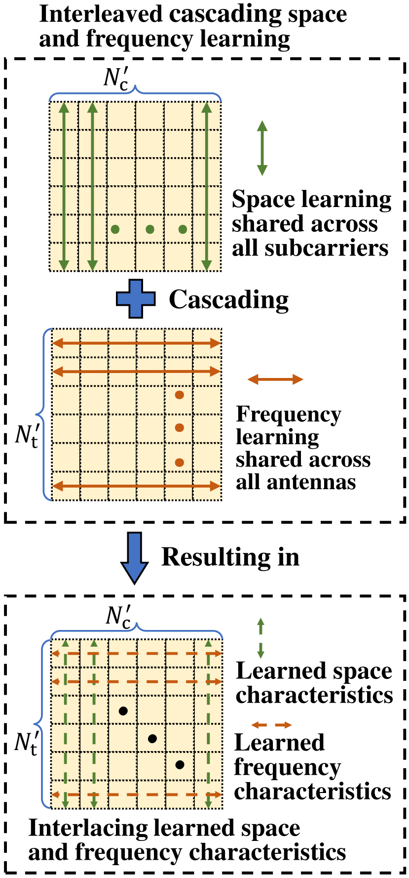
For any two columns of ${\bf{H}}\left[{:,m}\right],{\bf{H}}\left[{:,n}\right]$ $(\forall m,n\in\left\{{0,\ldots,{N_{\rm{c}}-1}}\right\})$, all antennas’ CSI of different subcarriers, although ${\bf{H}}\left[{:,m}\right],{\bf{H}}\left[{:,n}\right]$ have different frequency shifts $\Delta{f_{m}},\Delta{f_{n}}$, they still share the same space features $\left[{\vec{0},{{\vec{d}_{1}}},\ldots,{{\vec{d}_{{N_{\rm{t}}}-1}}}}\right]$ and the same large-scale features ${q_{\bf{H}}}(\cdot,\cdot)$. Similarly, for any two rows of ${\bf{H}}\left[{m,:}\right],{\bf{H}}\left[{n,:}\right](\forall m,n\in\left\{{0,\ldots,{N_{\rm{t}}-1}}\right\})$, all subcarriers’ CSI of different antennas, although there exists different space shift ${{\vec{d}_{m}}},{{\vec{d}_{n}}}$, they still share the same frequency features $[\Delta{f_{1}},\Delta{f_{2}},\ldots,\Delta{f_{{N_{\rm{c}}}}}]$ and the same large-scale features ${q_{\bf{H}}}(\cdot)$. To summarize, based on the shared large-scale channel features ${q_{\bf{H}}}(\cdot)$, shared space features $\left[{\vec{0},{{\vec{d}_{1}}},\ldots,{{\vec{d}_{{N_{\rm{t}}}-1}}}}\right]$ and shared frequency features $[\Delta{f_{1}},\Delta{f_{2}},\ldots,\Delta{f_{{N_{\rm{c}}}}}]$ interlaced couple, form the internal correlation of the whole CSI matrix.

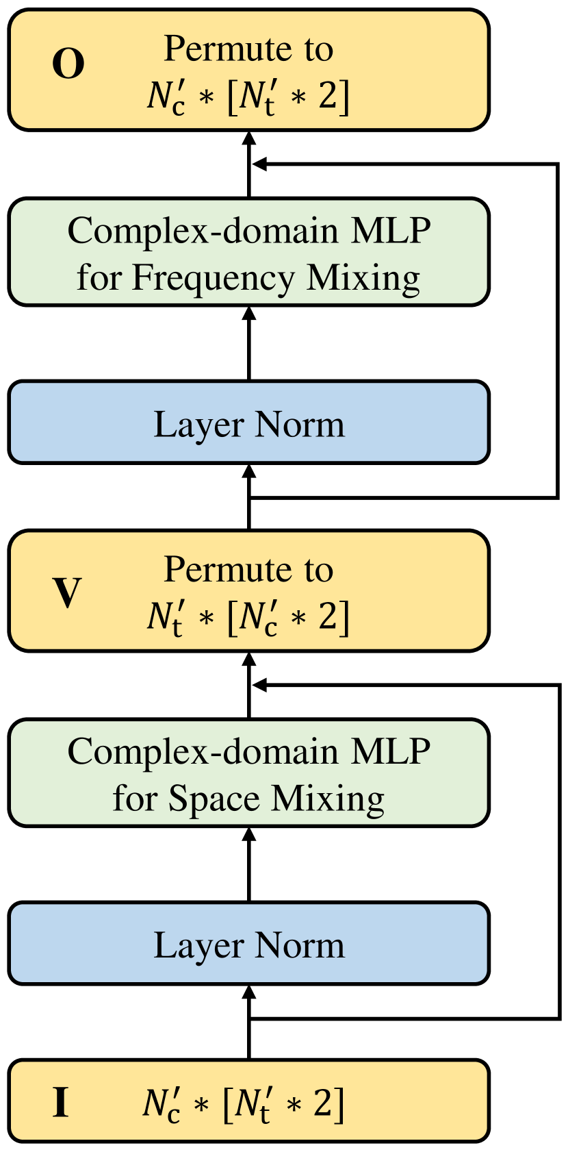
According to the revealed property, we propose an interleaved space and frequency learning approach for channel representation, as shown in Fig. 2(a). This approach first learns the space dimension, and this learning process is shared among all subcarriers, named as space mixing. This sharing of space learning process utilizes the sharing of space characteristics among all subcarriers. Then, the proposed approach learns the frequency dimension, and this learning process is also shared among all antennas, called frequency mixing. Similarly, this sharing of frequency learning process also utilizes the sharing of frequency characteristics among all antennas. The cascading of space mixing and frequency mixing interlaces the learned space and frequency characteristics, highly matching the revealed channel characteristics. In the neural network implement, similar to [6], we also introduce the residual connection and the layer normalization to keep the effectiveness and stability of training. Fig. 2(c) presents the specific learning module design, and the calculation process is as follows,

	$\displaystyle{\bf{V}}[i,:,:]$	$\displaystyle={\bf{I}}[i,:,:]+{\rm{SM}}({\rm{LN}}({\bf{I}}[i,:,:])),$
		$\displaystyle\leavevmode\nobreak\ \leavevmode\nobreak\ \leavevmode\nobreak\ \leavevmode\nobreak\ \leavevmode\nobreak\ \leavevmode\nobreak\ \leavevmode\nobreak\ \leavevmode\nobreak\ \leavevmode\nobreak\ \leavevmode\nobreak\ \leavevmode\nobreak\ \forall i\in\left[{0,1,\ldots,N_{\rm{c}}^{\rm{{}^{\prime}}}-1}\right],$		(13a)
	$\displaystyle{\bf{O}}[:,j,:]$	$\displaystyle={\bf{V}}[:,j,:]+{\rm{FM}}({\rm{LN}}({\bf{V}}[:,j,:])),$
		$\displaystyle\leavevmode\nobreak\ \leavevmode\nobreak\ \leavevmode\nobreak\ \leavevmode\nobreak\ \leavevmode\nobreak\ \leavevmode\nobreak\ \leavevmode\nobreak\ \leavevmode\nobreak\ \leavevmode\nobreak\ \leavevmode\nobreak\ \leavevmode\nobreak\ \forall j\in\left[{0,1,\ldots,N_{\rm{t}}^{\rm{{}^{\prime}}}-1}\right],$		(13b)

where $\bf{I}$ is the input, $\bf{O}$ is the output, $\bf{V}$ is the intermediate variable matrix, $\bf{I},\bf{O},\bf{V}$ are all of $N_{\rm{c}}^{{}^{\prime}}{\rm{\times}}{N_{\rm{t}}^{{}^{\prime}}}{\rm{\times 2}}$ size, and $\rm{SM}$, $\rm{FM}$, and $\rm{LN}$ are the abbreviation of space mixing, frequency mixing, and layer normalization, respectively. The computation in Eq. (13) completes a nonlinear representation of the input $\bf{I}$ through interleaved learning and yields an output $\bf{O}$ of the same size as $\bf{I}$.

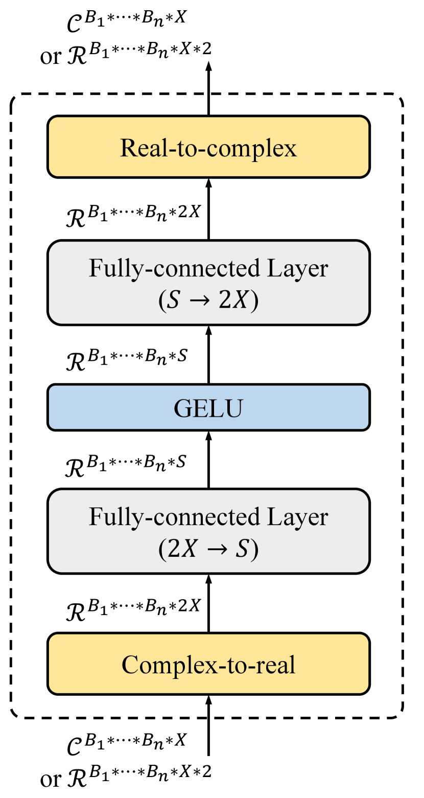
Considering that the channel characteristics are embodied in complex-valued data while the current mainstream DL platforms are based on real-valued operations, we design a complex-domain MLP (CMLP) module to specifically realize space mixing and frequency mixing. Fig. 2(d) shows the flowchart of CMLP, and the simplified calculation process can be written as follows,

$${\mathcal{C}^{X}/\mathcal{R}^{X*2}}\xrightarrow{{{\text{reshape}}}}{\mathcal{R}^{2X}}\xrightarrow{{{\text{MLP}}}}{\mathcal{R}^{2X}}\xrightarrow{{{\text{reshape}}}}{\mathcal{R}^{X*2}}/\mathcal{C}^{X},$$

(14)

where $\mathcal{C}$ represents complex-valued data and $\mathcal{R}$ represents real-valued data, $X$ refers to $N_{\rm{t}}^{{}^{\prime}}$ or $N_{\rm{c}}^{{}^{\prime}}$. $S$ in Fig. 2(d) is constant multiples of $X$. This method places the real and imaginary parts in the same neural layer for learning, which ensures the sufficient interaction of real and imaginary information better than treating the real and imaginary parts as separate channels. Moreover, this method recovers the complex dimension at the end to ensure that the next mixing can still be performed on the complex domain. Thus, the learning of the channel data can always remain in the complex domain, even if stacking multiple mixing layers. In summary, this subsection establishes an interleaved learning module, a CMixer layer, consisting of a cascade of a space-learning CMLP and a frequency-learning CMLP. It is suitable for channel representation learning since it is designed according to the channel’s physical properties.

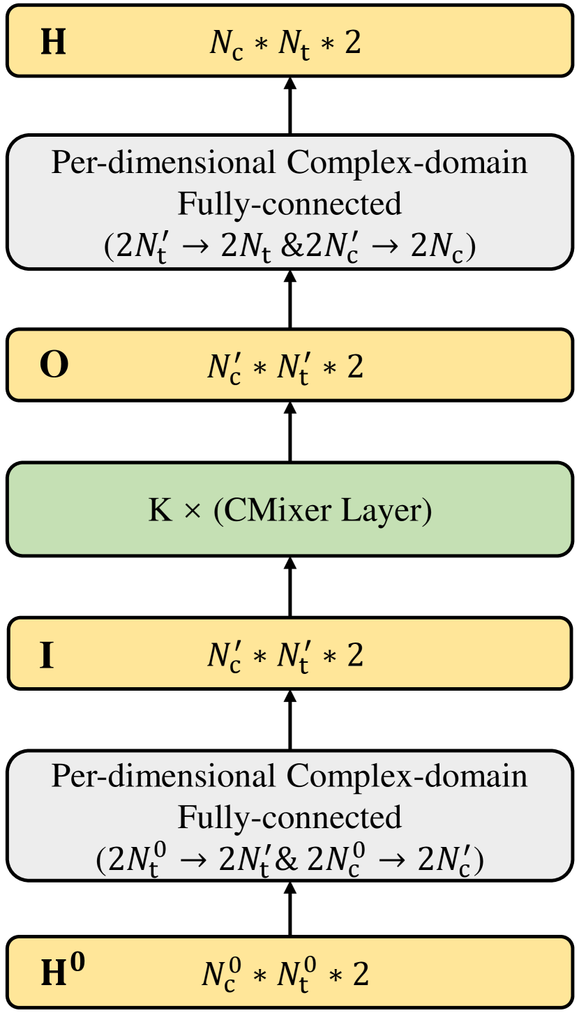
By stacking the above representation modules to enhance the nonlinearity and adding the necessary dimension mapping modules, the CMixer model is built for the channel mapping task. The network structure is shown in Fig. 2(b), and the calculation process is as follows. First, inputting the $N_{\rm{c}}^{0}{\rm{\times}}N_{\rm{t}}^{0}{\rm{\times 2}}$-size known channel to a $2N_{\rm{t}}^{0}\to 2N_{\rm{t}}^{{}^{\prime}}$ MLP layer and a $2N_{\rm{c}}^{0}\to 2N_{\rm{c}}^{{}^{\prime}}$ MLP layer to output a $N_{\rm{c}}^{{}^{\prime}}{\rm{\times}}N_{\rm{t}}^{{}^{\prime}}{\rm{\times 2}}$-size variable. This part yields $\mathcal{O}(N_{\rm{t}}^{0}N_{\rm{t}}^{{}^{\prime}}+N_{\rm{c}}^{0}N_{\rm{c}}^{{}^{\prime}})$ parameters and $\mathcal{O}(N_{\rm{t}}^{0}N_{\rm{t}}^{{}^{\prime}}N_{\rm{c}}^{0}+N_{\rm{c}}^{0}N_{\rm{c}}^{{}^{\prime}}N_{\rm{t}}^{{}^{\prime}})$ computation complexity. Then, inputting the $N_{\rm{c}}^{{}^{\prime}}{\rm{\times}}N_{\rm{t}}^{{}^{\prime}}{\rm{\times 2}}$-size variable to stacked $K$ CMixer layers and the output variable is still of $N_{\rm{c}}^{{}^{\prime}}{\rm{\times}}N_{\rm{t}}^{{}^{\prime}}{\rm{\times 2}}$ size. This part yields $\mathcal{O}(KN_{\rm{t}}^{{}^{\prime}}{S_{\rm{t}}}+KN_{\rm{c}}^{{}^{\prime}}{S_{\rm{c}}})$ parameters and $\mathcal{O}(KN_{\rm{t}}^{{}^{\prime}}{S_{\rm{t}}}N_{\rm{c}}^{{}^{\prime}}+KN_{\rm{c}}^{{}^{\prime}}{S_{\rm{c}}}N_{\rm{t}}^{{}^{\prime}})$ computation complexity. Finally, using a $2N_{\rm{t}}^{{}^{\prime}}\to 2{N_{\rm{t}}}$ MLP layer and a $2N_{\rm{c}}^{{}^{\prime}}\to 2{N_{\rm{c}}}$ MLP layer to mapping the previous output to ${N_{\rm{c}}}{\rm{\times}}{N_{\rm{t}}}{\rm{\times 2}}$-size variable, which is the whole MIMO-OFDM CSI. This part yields $\mathcal{O}(N_{\rm{t}}^{{}^{\prime}}{N_{\rm{t}}}+N_{\rm{c}}^{{}^{\prime}}{N_{\rm{c}}})$ parameters and $\mathcal{O}(N_{\rm{t}}^{{}^{\prime}}{N_{\rm{t}}}N_{\rm{c}}^{{}^{\prime}}+N_{\rm{c}}^{{}^{\prime}}{N_{\rm{c}}}{N_{\rm{t}}})$ computation complexity. Since $N_{\rm{t}}^{0}<{N_{\rm{t}}},N_{\rm{c}}^{0}<{N_{\rm{c}}}$, $N_{\rm{t}}^{{}^{\prime}}$ and ${S_{\rm{t}}}$ are constant multiples of $N_{\rm{t}}$, $N_{\rm{c}}^{{}^{\prime}}$ and ${S_{\rm{c}}}$ are constant multiples of $N_{\rm{c}}$, the total parameter scale of this model is $\mathcal{O}\left({KN_{\rm{t}}^{2}+KN_{\rm{c}}^{2}}\right)$ and the total computation complexity is $\mathcal{O}\left({KN_{\rm{t}}^{2}{N_{\rm{c}}}+KN_{\rm{c}}^{2}{N_{\rm{t}}}}\right)$. To train the model, mean square error (MSE) is used as the loss function, which can be written as

$$\mathrm{Loss}(\Theta)=\frac{1}{N}\sum\limits_{num=1}^{N}\left\|{{{{\mathbf{H}}}_{num}}-{{\widehat{\mathbf{H}}}_{num}}}\right\|_{2}^{2},$$

(15)

where $\Theta$ is the parameter set of the proposed model, $N$ is the number of channel samples in the training set, and $\|\cdot\|_{2}$ is the Euclidean norm. In addition, $\Theta$ can be updated through the existing gradient descent-based optimizers, such as the adaptive momentum estimation (Adam) optimizer.

In this work, we use the open-source DeepMIMO dataset of ‘O1’ scenario at 3.5GHz [7] for the simulation experiment. The bandwidth is set as 40MHz and divided to 32 subcarriers, the BS is equipped with a uniform linear array (ULA) consisting of 32 antennas. The user area is chose as R701-R1400. 50000 channel samples are randomly sampled from the dataset and divided into the training set and testing set with a ratio of 4:1. In addition, for intuitive performance evaluation, we use two existing typical DL-based channel mapping schemes as benchmarks. One is the MLP method [2], using a pure MLP network to learn the mapping function. The other is the Res_CNN method [4], using a CNN with residual connection as the network structure. Also, the model and training settings are summarized in Table I.

Moreover, we use normalized MSE (NMSE) and cosine correlation $\rho$ [8] as the performance indices, which are defined as follows:

$$\mathrm{NMSE}=\mathbb{E}\left\{{\frac{{\left\|{{\mathbf{H}}-\widehat{\mathbf{H}}}\right\|_{2}^{2}}}{{\left\|{\mathbf{H}}\right\|_{2}^{2}}}}\right\},$$

(16)

and

$$\rho{\rm{=}}{\mathop{\mathbb{E}}\nolimits}\left\{{\frac{1}{{{N_{c}}}}\sum\limits_{m=1}^{{N_{c}}}{\frac{{|{{\widehat{\bf{h}}}_{m}}^{H}{{\bf{h}}_{m}}|}}{{||{{\widehat{\bf{h}}}_{m}}|{|_{2}}||{{\bf{h}}_{m}}|{|_{2}}}}}}\right\},$$

(17)

where the ${\bf{h}_{m}}/{\widehat{\bf{h}}}_{m}$ is the CSI of $m$-th subcarrier, i.e. the $m$-th columon of the CSI matrix $\mathbf{H}/\widehat{\mathbf{H}}$.

We first evaluate the mapping performance of the proposed CMixer and use various mapping settings to ensure the universality of evaluation results. The known channel size, the $\Omega$ in Eq. (4), is set as 4×4, 5×5, 6×6 and 7×7 (antennas × subcarriers). Table II shows the mapping performance of proposed scheme and benchmarks. Compared with benchmarks, the proposed CMixer provides 4.6~10dB gains in NMSE and 5.7~9.6 percentage points gain in $\rho$ under same known channel size, or reduces required known channel size by up to $67.3\%(1-16/49)$ under same and even better accuracy.

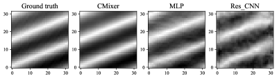
Further, Fig. 3 shows the mapping results of the different schemes on a random channel sample using grayscale visualization (Known channel size is 5 antennas × 5 subcarriers). It can be intuitively seen that the mapping channel based on CMixer is closer to the true channel than based on benchmarks. In summary, the above experimental results reflect the effectiveness and superiority of the proposed CMixer on the channel mapping task.

Complex-domain computation and interleaved learning are the two typical features of the proposed CMixer model. The performance evaluation in Section IV-B illustrates the superiority of the scheme as a whole, and this subsection evaluates the value of these sub-modules through ablation studies. These ablation experiments are all conducted under the known channel of 5 antennas × 5 subcarriers.

We first evaluate the necessity of using CMLPs. We replace the proposed CMLPs with vanilla MLPs. The specific ablation operation is changing the $2X\to S\to 2X$ calculation (CMLP) to the $2\left({X\to S\to X}\right)$ calculation (MLP with real and imag parallelism), remaining the same computation complexity, $4XS$, to ensure fairness. Table III shows the results of this ablation. Not using the CMLPs in either space mixing or frequency mixing leads to performance degradation. This phenomenon demonstrates the advantages of CMLPs in the representation learning of complex-valued channel data.

Then, we also evaluate what leads to the effectiveness of the proposed interleaved learning and whether it exactly stems from the unique interlaced space and frequency characteristics in the channel. Specifically, we shuffle the element order in the channel matrix in a way that remains/loses interlaced space and frequency characteristics and use the CMixer to learn the new matrix as the representation output. The first shuffle mode is named as ‘interlaced shuffle’ and written as,

$${{{\bf{H}}_{{\rm{interlaced}}}}={{\bf{P}}^{{N_{\rm{t}}}\times{N_{\rm{t}}}}}{{\bf{H}}^{{N_{\rm{t}}}\times{N_{\rm{c}}}}}{{\bf{P}}^{{N_{\rm{c}}}\times{N_{\rm{c}}}}},}$$

(18)

where each $\bf{P}$ represents a permutation matrix. In this way, the new channel matrix ${{\bf{H}}_{{\rm{interlaced}}}}$ has different space and frequency characteristics from the original channel ${\bf{H}}$, but its space and frequency characteristics are still interlaced coupled since its each row or column still respectively corresponds to certain antenna or subcarrier. The other shuffle mode is named as ‘non interlaced shuffle’ and written as,

$${{{\bf{H}}_{{\rm{non}}-{\rm{interlaced}}}}={\rm{vec}}^{-1}\left({{{\bf{P}}^{{N_{\rm{t}}}{N_{\rm{c}}}\times{N_{\rm{t}}}{N_{\rm{c}}}}}{\rm{vec}}\left({{{\bf{H}}^{{N_{\rm{t}}}\times{N_{\rm{c}}}}}}\right)}\right),}$$

(19)

where ${\rm{vec}}(\cdot)$ denotes the transposition of a matrix into a vector and ${\rm{vec}}^{-1}(\cdot)$ is the reverse process of ${\rm{vec}}(\cdot)$. In this shuffle mode, the row or column of ${{\bf{H}}_{{\rm{non}}-{\rm{interlaced}}}}$ does not necessarily correspond to certain antenna or subcarrier. Thus, the space and frequency characteristics are no longer coupled in an interlaced manner. Note that the above two kinds of new channel matrix ${{\bf{H}}_{{\rm{non}}-{\rm{interlaced}}}},{{\bf{H}}_{{\rm{interlaced}}}}$ and the original channel matrix ${\bf{H}}$ are identical in element content and only differ on the data structure. We use various random permutation matrices for experiments, and the statistical results are shown in Table IV. The proposed CMixer can effectively represent ${{\bf{H}}_{{\rm{interlaced}}}}$ with interlaced space and frequency characteristics while is severely degraded in representing ${{\bf{H}}_{{\rm{non}}-{\rm{interlaced}}}}$ without the interlaced characteristics. This phenomenon illustrates that the excellent performance of the proposed interleaved space and frequency learning indeed draws on the physical properties rather than relying exclusively on data fitting. The CMixer model’s performance gains come from the design inspired by channel characteristics.

References

- [1] Z. Chen, Z. Zhang, and Z. Yang, “Big AI models for 6G wireless networks: Opportunities, challenges, and research directions,” arXiv preprint arXiv:2308.06250, 2023.
- [2] M. Alrabeiah and A. Alkhateeb, “Deep learning for TDD and FDD massive MIMO: Mapping channels in space and frequency,” in 2019 53rd Asilomar Conference on Signals, Systems, and Computers, 2019, pp. 1465–1470.
- [3] M. Soltani, V. Pourahmadi, A. Mirzaei, et al., “Deep learning-based channel estimation,” IEEE Communications Letters, vol. 23, no. 4, pp. 652–655, 2019.
- [4] L. Li, H. Chen, H.-H. Chang, et al., “Deep residual learning meets OFDM channel estimation,” IEEE Wireless Communications Letters, vol. 9, no. 5, pp. 615–618, 2020.
- [5] Z. Chen, Z. Zhang, Z. Xiao, et al., “Viewing channel as sequence rather than image: A 2-D Seq2Seq approach for efficient MIMO-OFDM CSI feedback,” IEEE Transactions on Wireless Communications, vol. 22, no. 11, pp. 7393–7407, 2023.
- [6] I.O. Tolstikhin, N. Houlsby, A. Kolesnikov, et al., “MLP-Mixer: An all-MLP architecture for vision,” Advances in Neural Information Processing Systems, vol. 34, pp. 24261–24272, Dec. 2021.
- [7] A. Alkhateeb, “DeepMIMO: A generic deep learning dataset for millimeter wave and massive MIMO applications,” arXiv preprint arXiv:1902.06435, 2019.
- [8] C.-K. Wen, W.-T. Shih, and S. Jin, “Deep learning for massive MIMO CSI feedback,” IEEE Wireless Communications Letters, vol. 7, no. 5, pp. 748–751, Oct. 2018.