Chaos and unpredictability in evolutionary dynamics in discrete time
Abstract
A discrete-time version of the replicator equation for two-strategy games is studied. The stationary properties differ from those of continuous time for sufficiently large values of the parameters, where periodic and chaotic behavior replace the usual fixed-point population solutions. We observe the familiar period-doubling and chaotic-band-splitting attractor cascades of unimodal maps but in some cases more elaborate variations appear due to bimodality. Also unphysical stationary solutions can have unusual physical implications, such as the uncertainty of final population caused by sensitivity to initial conditions and fractality of attractor preimage manifolds.
pacs:
87.23.Kg, 05.45.Ac, 05.45.GgEvolutionary dynamics deals with a generic situation in which individuals interact and reproduce according to the result of that interaction, which in turn depends on the composition of the population Nowak (2006); Hofbauer and Sigmund (1998, 2003). This feedback loop gives rise to highly non trivial phenomena, that have attracted the interest of the physics community from the dynamical systems Traulsen et al. (2004, 2005); Roca et al. (2006); Galla (2009) , statistical mechanics Berg and Engel (1998); Szabó and Hauert (2002); Flor´ıa et al. (2009) and extended systems Szabó and Fáth (2007); Castellano et al. (2009); Roca et al. (2009); Perc and Szolnoki (2010) viewpoints. A particularly important class of problems is encompassed by the family generically referred to as replicator dynamics Taylor and Jonker (1978); Maynard Smith (1982); Schuster and Sigmund (1983). If is the frequency of type , is the frequency vector describing the population as a whole, and the interaction is given by the payoff matrix , then is the expected payoff for an individual of type and is the average payoff of the population. Assuming that the per capita rate of growth is given by the difference between the payoff for type and the average payoff in the population, we arrive at the replicator equation
| (1) |
Other forms have been proposed for this equation, which, e.g., include a denominator given by the average global payoff (albeit in this case the orbits of the resulting equation are the same) or other modifications (see, e.g., Hofbauer and Sigmund (2003); see also Binmore et al. (1995) and references therein). However, Eq. (1) is the one most often studied, and therefore we will stick to this form in the following.
Among the very many nonlinear phenomena exhibited by the replicator equation, the appearance of chaotic dynamics has been studied in a number of papers. The Poincaré-Bendixson theorem Schuster (1988) establishes that chaos can only arise in a continuous dynamical system (specified by differential equations) if it has three or more dimensions. Accordingly, Skyrms Skyrms (1992) showed that chaos does not exist for three types (also referred to as strategies) and gave examples of chaotic dynamics on strange attractors with four strategies. Further examples were provided in Nowak and Sigmund (1993); Chawanya (1995). Subsequently, Sato et al. Sato et al. (2002) found both hamiltonian and non-hamiltonian chaos in a three-type version of the rock-scissors papers game Nowak (2006); Maynard Smith (1982) by introducing asymmetry (payoffs depend on being the first or the second to interact).
In this letter we show that replicator dynamics does lead to chaos in games with only two types when the discretized version of the equation is considered, i.e.,
| (2) |
where is the composition of the population at time . We will refer to Eq. (2) in what follows as the replicator mapping and can be seen as arising from situations in which changes per generation are not necessarily small Maynard Smith (1982). We note that this is one of several existing discrete versions of the replicator equations Binmore et al. (1995) and in particular it has been considered in Dekel and Scotchmer (1992); Cabrales and Sobel (1992). As we will see below, the relevance of this result goes beyond the observation of chaos in low-dimensional systems under the required circumstances: Indeed, the occurrence of chaos as well as of periodic trajectories gives rise to unexpected behavior in well-known games for which so far only rest points have been reported.
We will focus on the generic two-strategy game given by the payoff matrix
|
(3) |
where payoffs for the row player are indicated. This choice encompasses several of the most important dilemmas arising in both biological and social applications.
According to the values of and , we have four basic social dilemmas: When and (upper-right region in Fig. 1) we obtain the Snowdrift game (also known as Chicken or Hawk-Dove) Sugden (1986), which represents a situation in which the best thing is to do the opposite of what the opponent does (i.e., it is an anti-coordination game). The region and (lower-left region) corresponds to the Stag Hunt game Skyrms (2003), a coordination game in which what is best is to do as the other player does. Finally, the other two regions define the Prisoner’s Dilemma ( and , lower-right) Axelrod (1984), where D is the best option no matter what the opponent chooses, and the Harmony game Licht (1999), with C being now the best strategy. In general, practically all the studies published on this two-parametric representation of social dilemmas deal with the square (referred to as “basic square” in what follows) as this is deemed enough to understand the four main classes of games, although other special regions can be identified (see, e.g., Hauert (2002)). With these payoffs, the replicator mapping given by Eq. (2) becomes
| (4) |
where now stands for the proportion of C-strategists in the population (the frequency of D-strategists being obviously ).
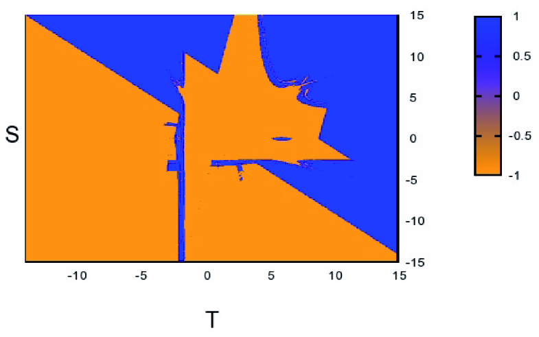
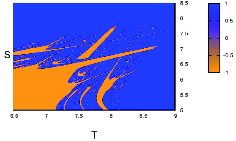
To begin our analysis, we first consider the Lyapunov exponent of the mapping in Eq. (4) as a function of and , plotted in Figure 1. As can be seen from the figure, below the diagonal the Lyapunov exponent is negative almost everywhere, whereas above the diagonal there is a region with intricate boundaries where the exponent remains positive, and outside that region it becomes negative. Interestingly, the basic square is contained in the region in which the Lyapunov exponent is negative. We recall that a negative Lyapunov exponent is indicative of periodic solutions and, as will be discussed below, periods do exist, although always outside the basic square, where only the well-known fixed-point solutions () are found. Perhaps this is the reason why all this new phenomenology has not been noticed before, and it indicates that capturing the richness of evolutionary game theory, when viewed in discrete time, demands the study of a larger payoff parameter region or, alternatively, of certain specific cases. In fact, as the zoom in Fig. 1 shows, the boundary between the chaotic and non-chaotic regions is very complicated, with fractal features, as it is regularly the case in dynamical systems. Another important remark is that in relation to game theory we have observed two types of chaos. There is non-physical chaos when in the chaotic region the variable becomes negative or takes values larger than 1, which are unphysical in so far it is the frequency of C-strategists and therefore must be bounded by 0 and 1; this takes place in the upper-left region, the Harmony game. On the other hand, in the Snowdrift game, we have observed physical chaos in the sense that the values of remain bounded within 0 and 1 for all times, and therefore trajectories represent actually realizable evolutions of populations. It is important to realize, however, that even non-physical chaos can be relevant in the sense that while trajectories become unphysical above 1 or below 0, the existence of chaos makes unpredictable in practice where any initial condition will end, i.e., to which of the two absorbing states or will become attached. Moreover, in case the chaotic motion takes place only around one of these two absorbing states, so that we know exactly in which of them the system will freeze, the time needed to reach the final configuration is sensitively dependent on the initial conditions and therefore unpredictable. These considerations hold in particular when is large and the system stays in the physical interval enough time before hitting a boundary: we have verified that when the initial condition is close to an unstable equilibrium (or repellor), this is actually the case.
In order to gain more insight on how the transition to chaos takes place, we have focused on the case and represented the Lyapunov exponent as a function of the new parameter . Figure 2 shows the behavior of the Lyapunov exponent as a function of . The upper plot clearly shows that both in the region where we found physical () or unphysical () behavior there is a well defined route to chaos. Furthermore, the unphysical region reproduces the period-doubling route to chaos characteristic of unimodal (one hump) maps, whereas in the physical region we have a different but not unrelated route that arises because of bimodality (two extrema) of the map when .
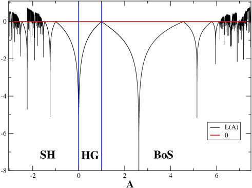
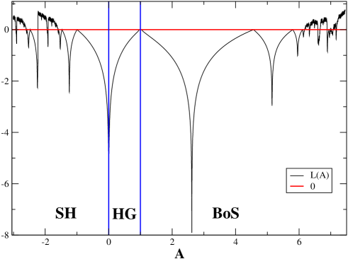
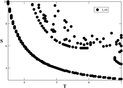
For small to moderate trajectories settle into periodic and chaotic attractors generated separately by each of the extrema of the map, but for sufficiently large trajectories spread and bounce between both extrema and converge to new periodic and chaotic attractors. This is the reason why in Fig. 2 the Lyapunov exponent for large differs from the familiar unimodal pattern shown when . The lower panel of Fig. 2 shows the effect on the Lyapunov exponent of additive noise in Eq. (4). As expected, we observe a gradual smearing out of the fine structure due to the removal of periodic and chaotic-band attractors with increasing noise amplitude . This amplitude fixes the largest period and number of bands present, , giving rise to the so-called bifurcation gap Crutchfield et al. (1982). Importantly, the chaotic behavior is not restricted to the diagonal: As shown in Fig. 3 the boundary between the fixed point solution (the same as in the continuous time replicator equation) and the period-two orbits takes a hyperbole-like shape. Then, moving outwards in the plane, boundaries between period two and period four orbits appear, and so on. It is important to note that the plane region usually considered in these studies, namely the basic square (bottom left of, and out of, Fig. 3) contains only fixed point solutions, i.e., in that region the continuous replicator equation and the discretized version we are studying here lead to the same dynamical behavior.
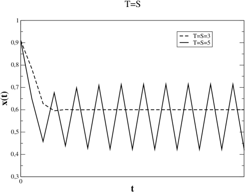
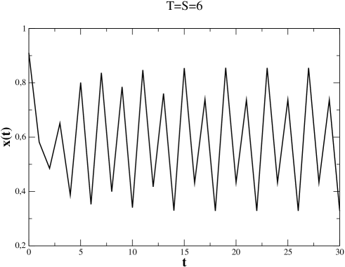
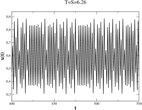
Finally, Fig. 4 illustrates the dynamics typically found in the route to chaos along the diagonal () of the region with physical behavior. As is increased, we observe the convergence to the fixed point, continuous-like solution, or to periodic solutions until reaching chaos (bottom panel of Fig. 4). This route to chaos appears an infinite number of times along the family of attractors generated by unimodal maps within periodic windows that interrupt sections of chaotic attractors. In the opposite parameter direction, a route out of chaos accompanies each period-doubling cascade by a chaotic band splitting cascade Schuster (1988). Bimodal maps with a minimum and a maximum (as in the case ) display interesting variations of these attractor cascades.
In summary, we have studied a discretized version of the replicator dynamics and found that there are large regions of the parameter space of the typical social dilemmas for which considering discrete time leads to behavior largely different from the continuous one. Indeed, beyond the restricted region which has been analyzed before, we observe that as the parameters and increase, periodic () and chaotic dynamics occurs. This is an important difference with respect to the continuous time dynamics, for which only fixed point solutions are found. We have also classified those novel behaviors as physical and unphysical, depending on whether the values of the concentration of C-strategists remain in or spread beyond the boundaries of this interval. In the physical case, periodic solutions imply that C and D strategists vary periodically in frequency, the state of the system being generally mixed, containing both types of individuals. Such cycles have only been observed in the continuous replicator dynamics for rock-scissors-paper games, i.e., games with three strategies Nowak (2006); Hofbauer and Sigmund (1998, 2003). The occurrence of chaotic behavior adds unpredictability to the features of the system, in complete contrast with the predictive character of the continuous case. On the other hand, periodic or chaotic behavior, even being unphysical, still has important consequences: In the time interval in which the trajectory is still contained in , in the chaotic region it turns out that it is not possible to predict whether, starting from a given initial condition, the system will end up in a population fully consisting of C- or D-strategists. We stress that our results may be relevant for real life applications, in many cases involving bacteria, animals or humans which are well described by social dilemmas that do not have well-determined payoffs, and often take place in discrete time. In principle, it is possible to test our ideas in experimental setups, at least with human volunteers, by setting properly chosen payoffs and interactions as discrete events. Clearly, the appearance of periodic orbits and chaos is generic and will affect other strategic interactions when described by a discretized equation. Unimodal maps (obtained e.g., when ) show a rich self-affine structure of chaotic-band attractors interspersed by periodic windows within which multiple period-doubling and band-splitting cascades take place. Bimodal maps (obtained e.g., when ) display more elaborate attractor structures. These dynamical features manifest in the discrete-time evolutionary dynamics addressed here and translate into matching patterns of population behavior.
D. V. aknowledges a postdoctoral contract from Universidad Carlos III de Madrid. The stay of A. R. at Universidad Carlos III de Madrid was supported by a grant from the Ministerio de Educación y Ciencia (Spain). A. S. aknowledges grants MOSAICO and Complexity-NET RESINEE (Ministerio de Ciencia e Innovación, Spain) and MODELICO-CM (Comunidad de Madrid, Spain).
References
- Nowak (2006) M. A. Nowak, Evolutionary dynamics: exploring the equations of life (The Belknap Press of Harvard University Press, Cambridge, 2006).
- Hofbauer and Sigmund (1998) J. Hofbauer and K. Sigmund, Evolutionary Games and Population Dynamics (Cambridge University Press, Cambridge, 1998).
- Hofbauer and Sigmund (2003) J. Hofbauer and K. Sigmund, Bulletin of the American Mathematical Society 40, 479 (2003).
- Traulsen et al. (2004) A. Traulsen, T. Röhl, and H. G. Schuster, Phys. Rev. Lett. 93, 28701 (2004).
- Traulsen et al. (2005) A. Traulsen, J. C. Claussen, and C. Hauert, Phys. Rev. Lett. 95, 238701 (2005).
- Roca et al. (2006) C. P. Roca, J. A. Cuesta, and A. Sánchez, Phys. Rev. Lett. 97, 158701 (2006).
- Galla (2009) T. Galla, Phys. Rev. Lett. 103, 198702 (2009).
- Berg and Engel (1998) J. Berg and A. Engel, Phys. Rev. Lett. 81, 4999 (1998).
- Szabó and Hauert (2002) G. Szabó and C. Hauert, Phys. Rev. Lett. 89, 118101 (2002).
- Flor´ıa et al. (2009) L. M. Floría, C. Gracia-Lazaro, J. G. Gardeñes, and Y. Moreno, Phys. Rev. E 79, 026106 (2009).
- Szabó and Fáth (2007) G. Szabó and G. Fáth, Phys. Rep. 446, 97 (2007).
- Castellano et al. (2009) C. Castellano, S. Fortunato, and V. Loreto, Rev. Mod. Phys. 81, 591 (2009).
- Roca et al. (2009) C. P. Roca, J. Cuesta, and A. Sánchez, Phys. Life Rev. 6, 208 (2009).
- Perc and Szolnoki (2010) M. Perc and A. Szolnoki, BioSystems 99, 109 (2010).
- Taylor and Jonker (1978) P. D. Taylor and L. Jonker, Math. Biosci. 40, 145 (1978).
- Maynard Smith (1982) J. Maynard Smith, Evolution and the Theory of Games (Cambridge University Press, Cambridge, 1982).
- Schuster and Sigmund (1983) P. Schuster and K. Sigmund, J. Theor. Biol. 100, 533 (1983).
- Binmore et al. (1995) K. G. Binmore, L. Samuelson, and R. Vaughan, Games Econ. Behav. 11, 1 (1995).
- Schuster (1988) H. Schuster, Deterministic Chaos. An Introduction, 2nd revised ed. (VCH, Weinheim, 1988).
- Skyrms (1992) B. Skyrms, J. Logic Lang. Infor. 1, 111 (1992).
- Nowak and Sigmund (1993) M. A. Nowak and K. Sigmund, Proc. Natl. Acad. Sci. USA 90, 5091 (1993).
- Chawanya (1995) T. Chawanya, Prog. Theor. Phys. 94, 163 (1995).
- Sato et al. (2002) Y. Sato, E. Akiyama, and J. D. Farmer, Proc. Natl. Acad. Sci. USA 99, 4748 (2002).
- Dekel and Scotchmer (1992) E. Dekel and S. Scotchmer, J. Econ. Theory 57, 392 (1992).
- Cabrales and Sobel (1992) A. Cabrales and J. Sobel, J. Econ. Theory 57, 407 (1992).
- Sugden (1986) R. Sugden, The economics of rights, co-operation and welfare (Basil Blackwell, Oxford, 1986).
- Skyrms (2003) B. Skyrms, The Stag Hunt and Evolution of Social Structure (Cambridge University Press, Cambridge, 2003).
- Axelrod (1984) R. Axelrod, The Evolution of Cooperation (Basic Books, New York, 1984).
- Licht (1999) A. N. Licht, Yale J. Int. Law 24, 61 (1999).
- Hauert (2002) C. Hauert, Int. J. Bif. Chaos 12, 1531 (2002).
- Crutchfield et al. (1982) J. P. Crutchfield, J. Farmer, and B. A. Huberman, Physics Reports 92, 45 (1982).