Chaos on the conveyor belt
Abstract
The dynamics of a spring-block train placed on a moving conveyor belt is investigated both by simple experiments and computer simulations. The first block is connected by spring to an external static point, and due to the dragging effect of the belt the blocks undergo complex stick-slip dynamics. A qualitative agreement with the experimental results can only be achieved by taking into account the spatial inhomogeneity of the friction force on the belt’s surface, modeled as noise. As a function of the velocity of the conveyor belt and the noise strength, the system exhibits complex, self-organized critical, sometimes chaotic dynamics and phase transition-like behavior. Noise induced chaos and intermittency is also observed. Simulations suggest that the maximum complexity of the dynamical states is achieved for a relatively small number of blocks, around five.
pacs:
05.45.PqI Introduction
Spring-block type systems are successfully used for modeling various complex systems which exhibit self-organization. Usually, the static friction coefficients exceed the dynamical ones, in systems composed of two or more blocks connected by linear springs the coexistence of these friction types can lead to avalanches, nonlinear dynamics or Self-Organized Criticality (SOC) Bak1987 ; Bak1988 ; Bak1989 ; Carlson1989 .
Spring-block type models have broad interdisciplinary applications (for a recent review see Neda2009 ), and prove to be very useful in describing many complex phenomena in different areas of science. For example, they have been applied successfully to explain elements of the Portevin-Le Chatelier effect Lebyodkin1995 , the fragmentation obtained in drying granular materials in contact with a frictional surface Andersen1994a ; Andersen1994b ; Leung2000 , to understand the formation of self-organized nanostructures produced by capillary effects Jarai-Szabo2005 ; Jarai-Szabo2011 , to model magnetization processes and Barkhausen noise Kovacs2005 , to describe glass fragmentation Horvat2012 , and even for modeling highway traffic Jarai-Szabo2011a ; Jarai-Szabo2012 .
The first members of this model-family were presented in 1967 by R. Burridge and L. Knopoff Burridge1967 to explain the empirical Guttenberg-Richter law of the size distribution of earthquakes Gutenberg1956 . One of their original models (called BK model here) is composed of a chain of many blocks connected with springs and two planes, to model the sliding of tectonic plates (for a recent review see for example Kawamura2012 ). The blocks can slide with friction on the bottom surface and they are all connected by springs to the upper plane which is dragged with a constant velocity. This model presents stick-slip dynamics, and the size distribution of the slipping events exhibits a power-law scaling.
Since the pioneering work of Carlson et al. Carlson1989 ; Carlson1989a , the dynamics of the BK model has been investigated with several type of friction forces. In these studies both chaotic dynamics Xu1994 ; Ryabov1995 ; SousaVieira1999 ; Szkutnik2004 ; Erickson2011 and phase transition-like phenomena SousaVieira1993 have been reported.
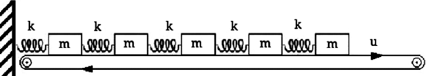
The system used here has also been proposed by Burridge and Knopoff Burridge1967 , and later it was referred as ”train model” SousaVieira1992 . As sketched in Fig. 1, a spring-block chain is placed on a platform (conveyor belt) that moves with constant velocity. The first block is connected by a spring to a static external point. As a result, due to the dragging effect of the moving platform, the blocks will undergo complex stick-slip dynamics.
The stick-slip dynamics of one block has been studied by analytical SousaVieira1994 ; Baumberger1995 ; Vasconcelos1996 ; Elmer1997 , numerical Baumberger1995 ; Vasconcelos1996 ; Elmer1997 ; Sakaguchi2003 and experimental methods Johansen1993 ; Baumberger1995 . The results for a chain composed of several blocks are contradictory from the point of view of self-organized criticality SousaVieira1992 ; SousaVieira1996 ; Vasconcelos1996 ; Chianca2009 . Undoubtedly, chaotic dynamics has been found in such systems by many authors SousaVieira1995 ; SousaVieira1999 ; Szkutnik2002 ; Erickson2008 . In these systems nonlinearity is introduced via friction forces, and several models have been studied from velocity-weakening SousaVieira1992 ; SousaVieira1994 ; SousaVieira1995 ; Szkutnik2002 to state-dependent Sakaguchi2003 friction forces. It has been shown that with velocity-weakening friction forces (and a constant static friction), the case of two blocks is the simplest autonomous spring-block system exhibiting chaos SousaVieira1995 . It was also argued, that for systems composed of many blocks, chaotic dynamics and SOC can coexist SousaVieira1996 .
It needs to be mentioned that a somewhat modified version of the train model has also been investigated, where in contrast with the former model, both the first and the last blocks are connected to static points. Additional springs are also introduced. This system also exhibits periodic and chaotic behavior Galvanetto1998 ; Galvanetto2002 .
Although the proposed problem has been thoroughly investigated for one, two and many blocks, we believe that a careful experimental and detailed simulation study for an intermediate number of blocks can reveal new and interesting dynamical complexity. Comparisons between analytical, numerical and experimental results exist mainly for the one block system. An exception is the work of Burridge and Knopoff Burridge1967 , where a chain of eight blocks was thoroughly investigated. The main purpose of their work was, however, to investigate the distribution of the potential energy released during avalanches, and they did not considered the problem from a dynamical systems view. Also, a general feature of previous numerical studies is that the model parameters and assumptions are arbitrarily chosen, and usually the only argument for this is to make the calculations or the numerical code simpler.
Here we consider an experimental setup composed of blocks, and computer simulations of a simple model for systems up to blocks. In contrast to previous works, the model parameters are realistically estimated from experimental measurements. We also incorporate the surface inhomogeneities of the conveyor belt by using a Coulomb type friction force varying stochastically about a mean. This feature appears to be essential since the temporal intermittency observed in the experiments cannot be recovered with only deterministic friction. A spring force with exponential cutoffs is used, to make the force profile more realistic and to avoid the collisions of the blocks with each other.
To the best of our knowledge this intermediate system size has not yet been investigated experimentally. The choice of intermediate system sizes is motivated by the expectation that this is the range where the theory of collective phenomena and of dynamical systems overlap and thus tools borrowed both from statistical mechanics and chaotic dynamics become both applicable. Despite the relatively small number of elements the system consists of, we surprisingly find a sharp phase transition-like behavior as a function of the conveyor belt velocity. Interestingly, as the size of the system is increased this transition becomes smoother, a phenomenon that can be understood through the intermittency that was revealed in this region. Tuning the level of disorder to a certain value, disorder induced phase transition-like behavior is also observed. We show that by using the Coulomb type friction forces this simple system exhibits a complex, chaotic dynamics accompanied by power-law type avalanche size distribution indicating SOC, noise induced intermittency and also noise induced chaos.
The work is structured as follows. First the used experimental setup is presented and the results are described for a chain of five blocks (Sec. II). In Sec. III the model is detailed. Simulation results (Sec. IV) without and with a disorder in the friction force are discussed. Finally, the influence of the number of blocks (up to ) on the observed dynamics is investigated (Sec. V) and final conclusions are drawn (Sec. VI).
II Experiments
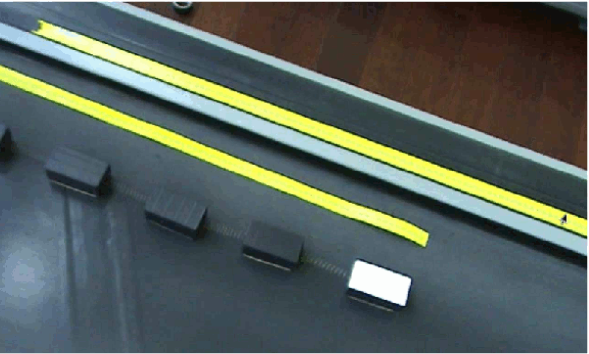
The experimental setup is sketched in Fig. 1. The chain is built by black wooden blocks of mass g, and of dimensions cm cm cm. The blocks are connected by steel springs of rest length cm and spring constant of N/m. The chain is placed on the conveyor belt of a treadmill (running machine) with adjustable speed. A digital camera is placed above the chain to record the dynamics of the blocks with fps (for a snapshot see Fig. 2). In order to make the last block clearly distinguishable from the others, and from the black colored conveyor belt, the top of this block is colored white.
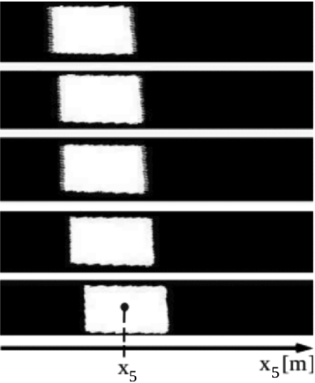
The video recordings are converted by a threshold operation into black and white image sequences as shown in Fig. 3. Then, the position of the last block is detected on these images. The length unit on the image can be determined using the image of a tape measure, which is placed next to the chain. Accordingly, the length of the chain as a function of time can be obtained automatically with a simple processing program.
The experiments were carried out with two values of the belt’s speed: m/s and m/s. The measured average values of friction forces in the experiment are N for static friction and N for kinetic friction. Thus, the ratio of the two types of friction forces is
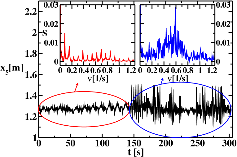
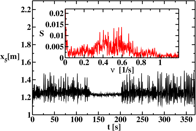
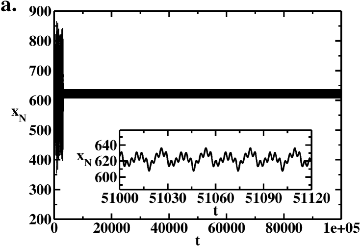
In both experiments the system is initialized with blocks sticking to the belt and with undeformed springs. Initially, the conveyor belt is at rest. After it is set in motion, length oscillations of very large amplitude occur on a time-interval up to s. In order to ensure that these initial transients are not considered and a kind of steady state has set in, a time-interval of s is discarded in the data processing. The recorded data for the position of the last block as a function of time is then analyzed. For the velocity m/s, the recorded data reveal (Fig. 4) two qualitatively different temporal behaviors. In the domain characterized by small amplitudes in , the dynamics of the system is nearly periodic, while in the domain of large amplitudes the last block exhibits a chaotic-looking behavior. We recall again, that the initial periodic-like behavior in this figure is not a result of the lasting transients, since before this, several chaotic-like regions were already present during the large amplitude bursts following the start of the conveyor belt.
The differences in the dynamics for these domains can be better understood from the Fourier Transforms (FT). We have thus computed separately the FT for the two well distinguishable regions (see Fig. 4). It is clearly observable that for the small amplitude interval the power spectrum of the FT has peaks at equal distances suggesting periodic dynamics, while in the chaotic region the power spectrum presents a quasi-continuous distribution.
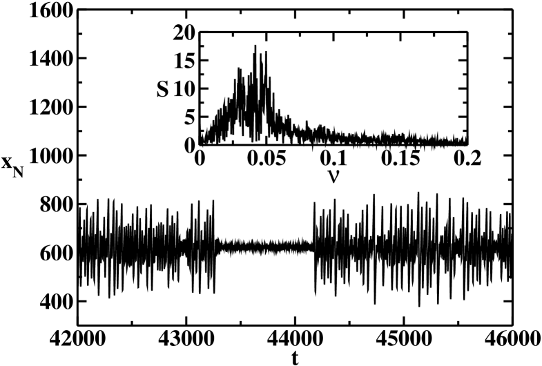
As can be seen in Fig. 5, for m/s the dynamics of the system is intermittent. In the first 125 seconds there are large ”avalanches” that result in a simultaneous movement of blocks (they slip and stick to the belt together). In this regime, the length of the chain evolves in time with fluctuations of large amplitudes. Then, without any external influence, the dynamical behavior changes abruptly, and for more than one minute the system remains in a nearly steady state, when all the blocks are slipping continuously relative to the belt. After this time interval, the behavior of the system looks chaotic again, of the type it was at the beginning of the recorded dynamics. The power-spectrum of the FT for the whole plotted interval is similar to the one observed for the chaotic regime for m/s.
III A simple model
The model contains the same elements (blocks and springs) as the experimental setup. The main challenge in the modeling effort is however the quantification of the friction and spring forces and the numerical integration of the equations of motion. Let us consider a chain formed by identical blocks of mass . The blocks are connected by identical springs of linear spring constant and undeformed length . As Fig. 1 indicates the motion of the blocks of the model is one dimensional and the transverse oscillations present in the experiment are thus neglected.
In the model, dimensionless units are taken. We have chosen these units so that , , and . The value for was chosen for the sake of an easier graphical visualization (spring length corresponding to pixels). Being motivated by the experiment, we cannot avoid using a nonzero rest length for the springs. In order to have these dimensionless values to correspond to the experimental situation, the units are chosen as: kg for mass, N/m for spring constant, and m for length. The units of the other quantities follow from dimensional considerations. The time, velocity and force units are thus, s, m/s, and N, respectively.
The equation of motion for the th block of the chain is written as
| (1) |
where and , respectively, and is the relative velocity of the block to the conveyor belt. The elastic force, , and the friction force, , are defined below.
The elastic force of any spring is linear, up to a certain deformation value, . For higher deformations, this dependence is assumed to become exponential, with an exponent bigger (in modulus) for negative deformations (see Fig. 6). Accordingly,
| (2) |
where we have chosen , for and for . With these choices the model is more realistic since the nonlinearity of spring forces is taken into account and collisions between blocks are avoided. At the same time the choice of parameters and is somewhat ad-hoc and we have not carried out a systematic change of them, other than the fact that the average chain lengths are thus comparable with those seen in the experiment with an error less than 10%.

According to a review of experimental results presented in Ref. Johansen1993 , ”the classical friction law, where the friction force is proportional to the load, will only exist in an average sense” and it is important to take into account that in many cases the friction is determined by surface asperities, which means that ”deterministic friction-velocity relations at best only exist in an average sense”. In Johansen1993 , the authors also argue that in the case of stick-slip dynamics on a plane surface, the friction forces may have normal distributions.
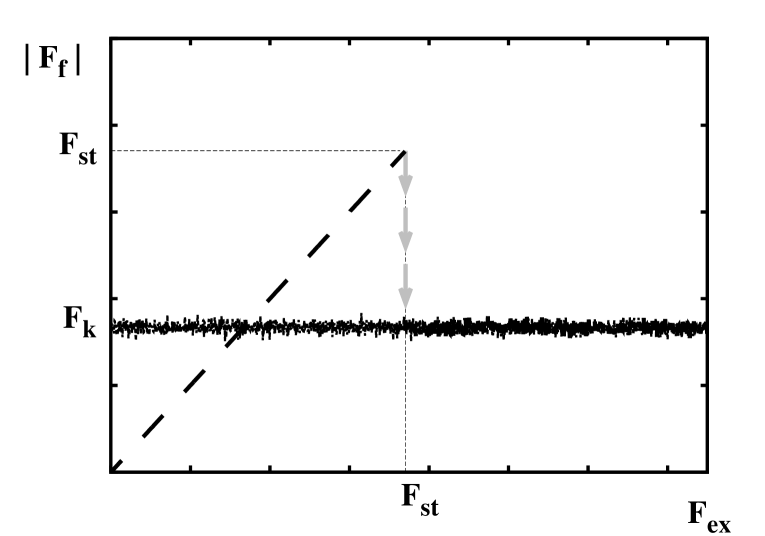
In the present paper Coulomb’s law of friction Bowden1954 is used with a noisy extension reflecting the surface irregularities. Both the static and kinetic friction forces are independent of velocity modulus. A block remains in a stick state until the resultant external force exceeds the value of the static friction force, . For higher external force values the block starts to slide in the presence of the kinetic friction force . We assume that, the ratio of the static and kinetic friction forces is constant. The friction force acting on the block depends both on , where is the signum function and is the block’s speed relative to the conveyor belt, and on the value of the resultant external forces acting on it. In our 1D setup, the friction force orientation is given only by its sign:
| (3) |
where and is the velocity of the block relative to the laboratory frame.
Since the surface of the conveyor belt is not perfectly smooth, the already mentioned argument of Ref. Johansen1993 is implemented by using randomly distributed friction forces. This is incorporated into the model by randomly generating a new static friction force value for every different position of the block relative to the belt. These random friction force values are generated according to a normal distribution with a fixed mean and standard deviation: . This standard deviation (together with the integration time-step, which is however the same for all simulations), will quantify the amount of disorder introduced in the model. Although the origin of the disorder is the spatial inhomogeneity of the belt’s surface, from the point of view of the dynamics the fluctuations of the friction force appear as temporal noise. We shall thus call as the noise strength.
The kinetic friction force value is always automatically updated together with the static friction force value, using their fixed ratio . As a result, both the kinetic and static friction forces will fluctuate in time during the sliding of the particular block. In Fig. 7 we illustrate the variation of the friction force as a function of the resultant external force for one stick-slip event. Such type of friction forces also proved to be useful for modeling highway traffic Neda2009 ; Jarai-Szabo2011a .
In order to use the same friction force value as in the experiments, in the dimensionless units the average value of the static friction force is . The ratio of the two types of friction forces is also chosen in agreement with the experiments as .
Computer simulations of the model start from initial conditions similar to the experimental ones. The blocks are placed on the belt with undeformed springs between them. At this initial setup the blocks are stuck to the belt which means that their initial velocity in the laboratory reference frame is equal to the conveyor belt’s constant velocity . Computer graphics is also used to visualize in real-time the dynamics of the blocks.
The numerical methods used to solve Newton equations (1) are presented in the Appendix. The time-step of integration is fixed to .
In order to characterize statistically the dynamics of the chain, a parameter measuring the fluctuation of the chain length in dynamical equilibrium is introduced. The chain’s length is determined by the position of the last block in the row. The disorder parameter is defined as the standard deviation of the coordinate compared to the time averaged length of the chain:
| (4) |
This quantity takes on large values for large fluctuations which explains the term disorder parameter. Among other relevant dynamical measures, this disorder parameter is investigated as a function of the belt velocity (Section IV.1.), the noise level (Section IV.2.), and the number of blocks (Section V.).
IV Simulation results
IV.1 Results without noise
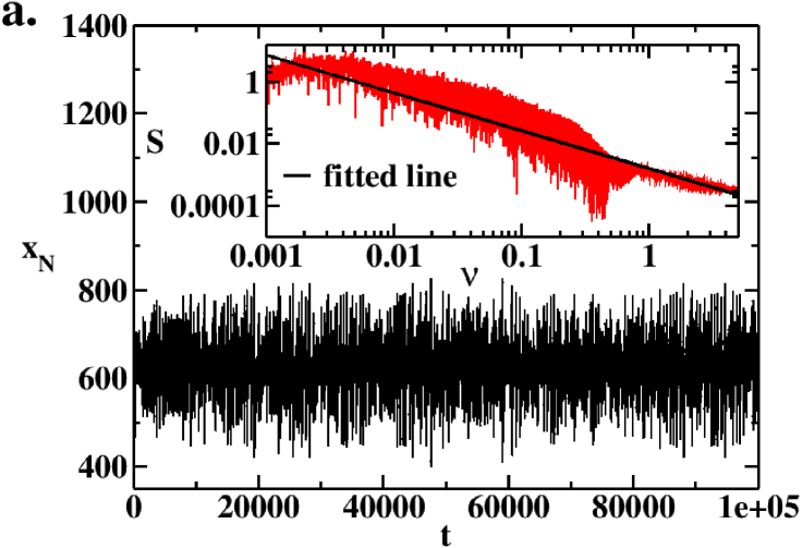
In the deterministic case, as the conveyor belt is started, the whole system moves together with the belt until the first block starts to slip. This slipping moment is determined simply by the value of the static friction force and the belt velocity . The block sticks again to the belt when its relative velocity becomes zero. After that the process starts again. For small belt velocities this kind of behavior characterizes all the blocks in a self-organized manner. Specifically, the blocks are slipping together and produce ”avalanches” of different sizes. Therefore, the length of the chain, defined by the position of the last block fluctuates as a function of time with largely varying amplitudes, as shown in Fig. 8.a.
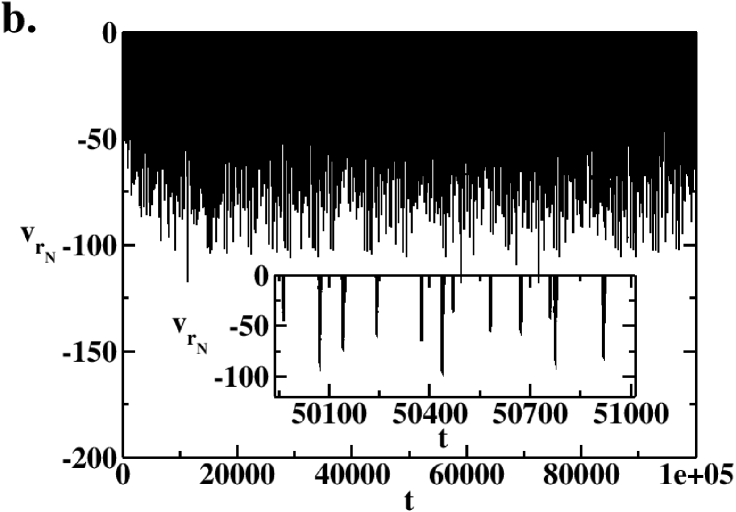
Furthermore, as shown in the inset of Fig. 8.a. the Fourier transform of the time series of exhibits a nearly power-law behavior with an exponent , suggesting a type stochastic behavior in the long time dynamics and a critically self-organized state. The relative velocity of the last block is zero, when the block is stuck to the belt. As the chain starts to slip, this relative velocity is rapidly increasing in absolute value as indicated in Fig. 8.b and it shows large fluctuations according to the inset of Fig. 8.b.
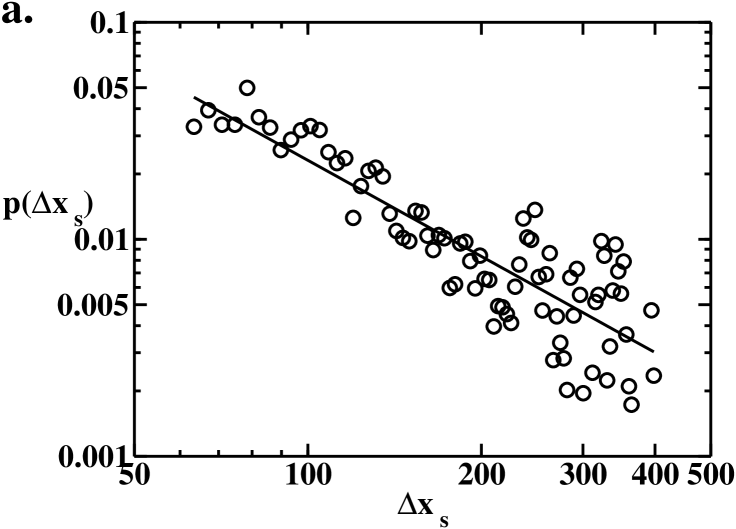
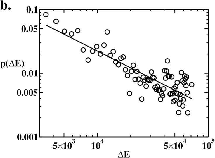
For a quantitative measure of avalanches, the slip size distribution for the last block is computed and shown in Fig. 9.a. The slip size is defined as the difference of the coordinates where the block starts to slip and when it stops relative to the belt. The obtained power law behavior confirms the presence of SOC, which appears here together with a chaotic dynamics. The distribution of the energies dissipated during avalanches is plotted in Fig. 9.b. The results indicates again a scaling (a sign for SOC-like behavior), although the exponent is different from the one obtained in the seminal work of Burridge and Knopoff Burridge1967 . This difference is a natural consequence of the different nature and size of the problems.
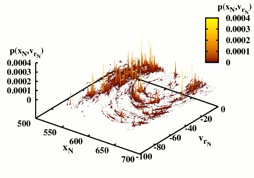
The existence of chaos is illustrated by Fig. 10, where the natural distribution on a Poincaré section is presented. This Poincaré section is projected onto the phase plane () of the last block, and obtained as the intersections of the system’s trajectory in the phase space with the plane defined by , considering only uni-directional crossings from right to left (). For a better view, the high probability states along the line (where the block is stuck to the belt) are not shown. In the full system of degrees of freedom the Poincaré section is -dimensional. Fig. 10 shows a projection of this on a plane. It is surprising that the natural distribution on this plane is similar in appearance (both in the shape of the support and of the rather irregular distribution) to that of the chaotic attractor of a driven one-dimensional system. This indicates that the chaotic attractor of the full chain is rather low-dimensional.
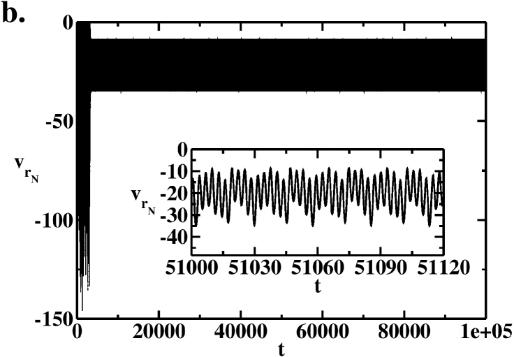
For higher values of the belt velocity, there are other possible scenarios as well. For instance, for the system exhibits an asymptotically periodic stick-slip dynamics, but for the behavior is aperiodic again. For the velocity interval permanent chaotic dynamics never occurs for the investigated parameters (see e.g. Fig. 11 for ) and the last block exhibits a continuous slip dynamics after a certain transient time. It can be seen in this figure that the system undergoes a transient chaotic behavior with a stick-slip dynamics, before reaching a periodic attractor.
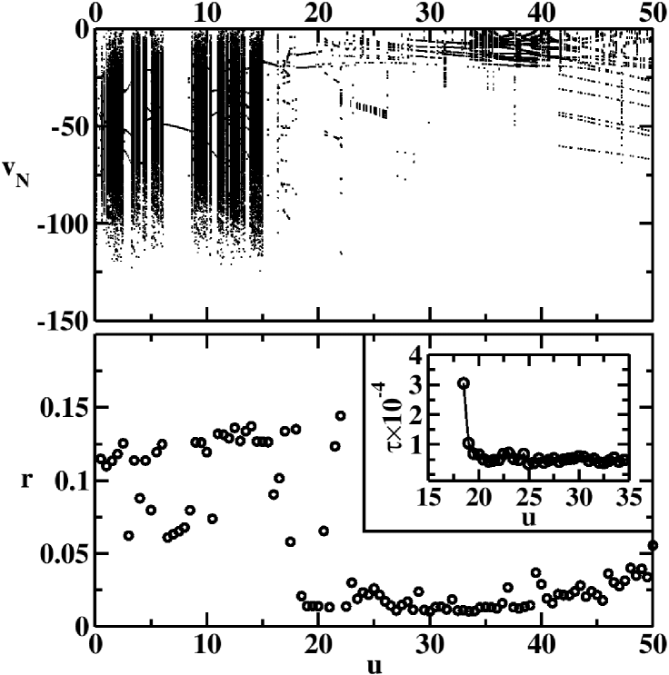
The bifurcation diagram plotted in the top panel of Fig. 12 summarizes all the cases described above. Here, the velocity of the last block is plotted as a function of the driving velocity in instances when the block goes through a fixed () position from the right. For every value of the control parameter the simulation is restarted from the declared initial position. To construct this plot, the computer simulations were run up to time units, discarding a transient time of .
Interestingly, the disorder parameter (4) allows for a difference to be made between these different dynamical behaviors. Results for are plotted on the bottom panel of Fig. 12. As expected, for asymptotic chaos the disorder parameter has a high value, and in the case of the periodic or quasi-periodic dynamics, it is much smaller. In the transition region () the value of falls from about to . This jump of nearly one order of magnitude indicates a relatively sharp dynamical phase transition-like behavior. The critical speed , defined as the midpoint of the transition region, which the phase transition-like behavior can be associated with, is . (Note that in the interval there are three outlier points in the lower panel of Fig. 12. These belong however to periodic attractors of large amplitudes rather than to chaotic cases.)
In the inset of Figure 12, the average lifetime of the chaotic transients preceding the periodic behavior is presented. This is measured using the method described in Ref Tel2008 . Looking at the simulation data, it can be seen that in the phase transition region the lifetime of transients grows considerable, a kind of critical slowing down can be observed. It can thus be concluded, that for (except for the periodic windows) the chaotic dynamics is permanent, while for it has a transient character. These transients were neglected in computing the disorder parameter, since the discarded transient time () is larger by more than two orders of magnitude than the average lifetime of the transients.
IV.2 Results in the presence of noise
As described earlier, the two friction forces are linked by the relation , and the values of are randomly updated for each new position of the blocks on the conveyor belt. The distribution of has a standard deviation and a mean value .
First, a relatively low level of noise is considered (see Fig. 7). In this case, the phase transition-like behavior remains almost unchanged. This is clearly visible in the plots of Fig. 13. The periodic windows present for (top panel of Fig. 12) disappear, however, and consequently the disorder parameter has less fluctuations in the chaotic regime. The noisy bifurcation diagrams of Fig. 14 also illustrate the disappearance of the periodic windows as increases.
For belt velocity and small noise levels, the asymptotic periodic dynamics is reached after a transient chaotic behavior. This is possible if a non-attracting chaotic set (chaotic saddle) and periodic attractors coexist (see for example Tel2006 ; *Lai2011). Beyond a critical noise level , the chaotic transients turn into a permanent chaotic dynamics. This is called noise induced chaos IANSITI1985 ; HERZEL1987 ; BULSARA1990 ; HAMM1994 ; Tel2008 . Based on the results plotted in the inset of Fig. 14 the critical noise strength necessary to obtain noise induced chaos is estimated as .
By increasing the noise level in the friction force, the critical speed , for which a phase transition-like behavior occurs, increases with as suggested by Fig. 13.
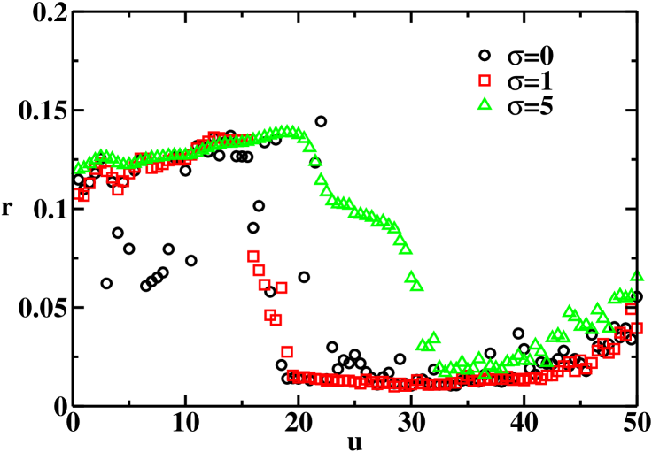
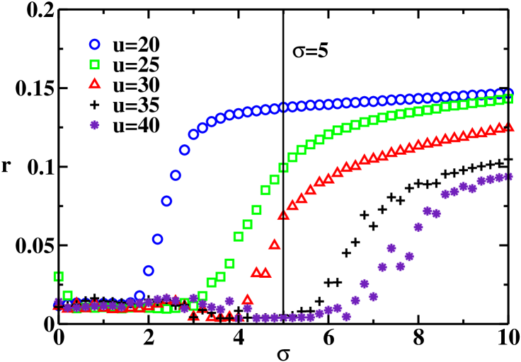
Turning the problem around, in Fig. 15 we plot the disorder parameter as a function of the noise level for intermediate velocities . In the whole range a noise induced phase transition-like behavior emerges. Moving away from , the sharp transition becomes more smooth and the transition point in is shifted toward higher noise levels. A possible explanation of this effect is that for higher velocities a higher noise level is needed to kick the system out from the basin of attraction of the periodic attractor.
The model is able to reproduce the intermittent behavior observed in the experiment and presented in Fig. 4. For example, considering , and belt velocities in the phase transition-like region, the system exhibits an intermittent dynamics (Fig. 16). Since such intermittency is not present without noise, this phenomena is called noise induced intermittency Tel2006 ; *Lai2011 in the chaos literature. This can happen again only if a chaotic saddle exists in the deterministic system Tel2006 ; *Lai2011.
We note that the critical speed is found to be which corresponds in dimensional units to m/s. Experimentally we have found intermittency at m/s and m/s which should belong to velocities close to the critical value. In view of the simplicity of the model this order of magnitude agreement is satisfactory.
The disorder parameter can be computed also for the experimental time series of of Figs. 4 and 5. The results are: and for m/s and m/s, respectively. The values corresponding in the model to these dimensional velocities are: and , respectively, again in an order of magnitude agreement with the experiments.
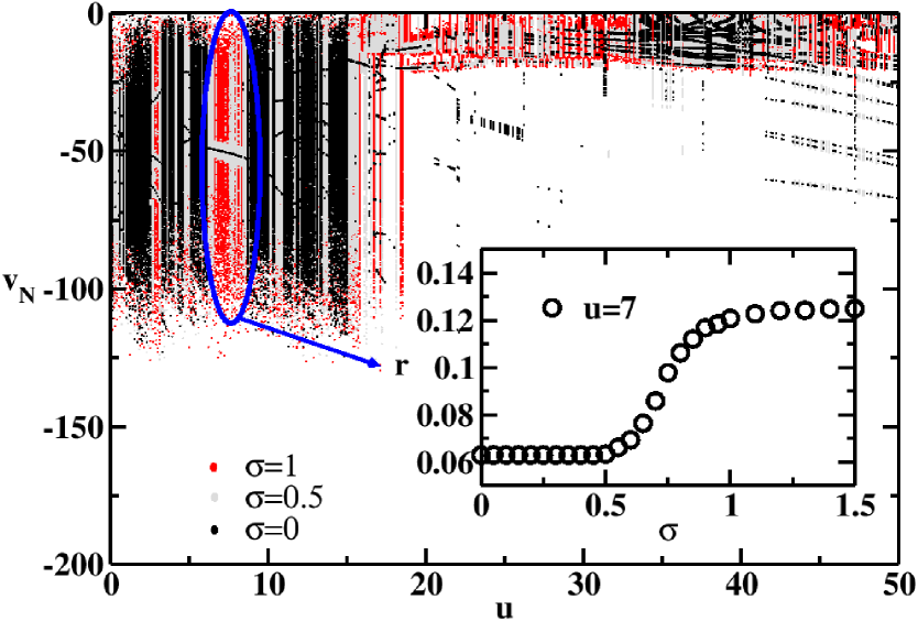
Another facet of the effect of noise is shown in Fig. 17, where the natural distribution is projected to the bifurcation diagram defined in Sec. IV.1. The consecutive graphs are results for increasing noise levels. From these plots we learn that for all the periodic windows in the interval disappear, but the phase transition point hardly changes. As is increased further, the sharp phase transition-like behavior transforms into a smoother one (see Fig. 17.c). For the dynamics of the system is dominated by noise (Fig. 17.d).
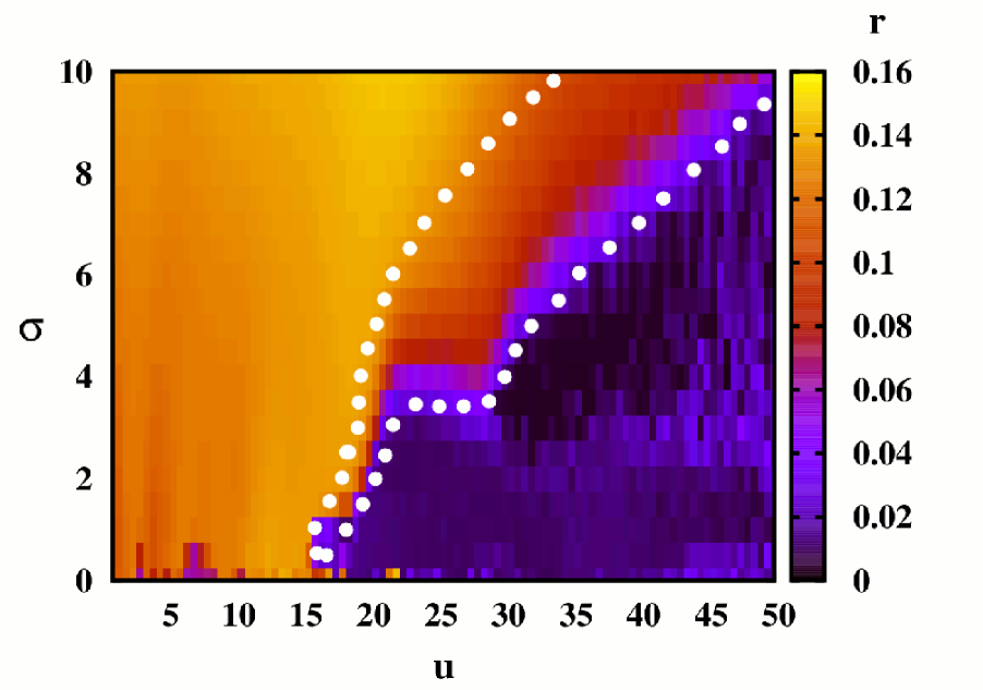
The results regarding the phase transition-like behavior are summarized in Fig. 18 by a detailed map of the parameter space . Figures 13 and 15 correspond to sections of this map along the horizontal and vertical axes, respectively. The range where the system exhibits noise induced intermittency is enclosed by white dots. The fact that this range does not reach the line shows, that intermittency cannot be recovered with purely deterministic friction forces. As the level of noise is increased, this region becomes abruptly wider for . This can be interpreted as the critical noise strength below which the phase transition-like region remains sharp, and if this is exceeded, the transition becomes smoother. In the view of all these observations we conclude that the noise strength corresponding to the experiments is about .
V Finite size effects
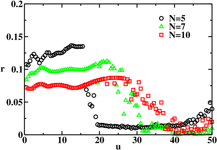
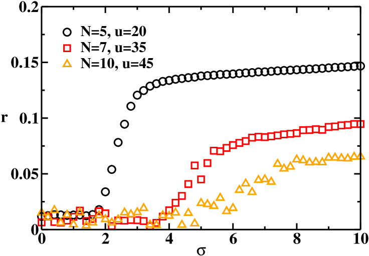
We can now briefly discuss the influence of the system size on the observed phase transition-like phenomena. We know from statistical physics that the observed phase transitions become sharper as the system size is increased. Although the investigated system is a non-equilibrium dynamical system and not a system in thermal equilibrium, one might expect that the phase transition-like behavior sharpens for larger system sizes. In our system, however, the opposite happens. As shown in Fig. 19 for increasing system sizes, the sharp phase transition-like behavior is transformed into a smoother and smoother one, the transitional region broadens with .
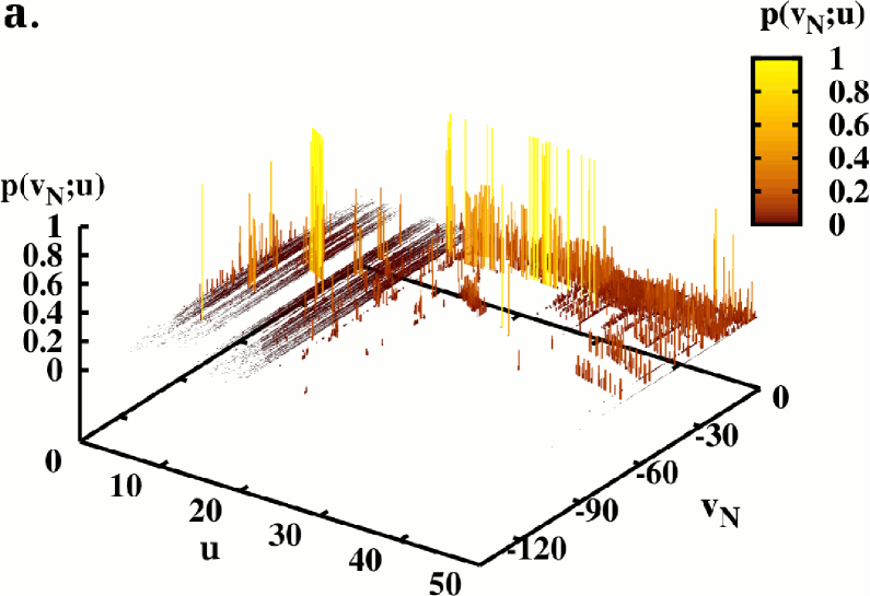
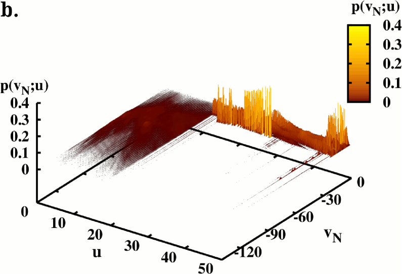
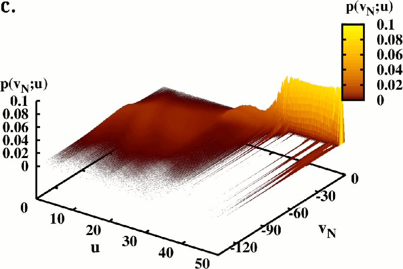
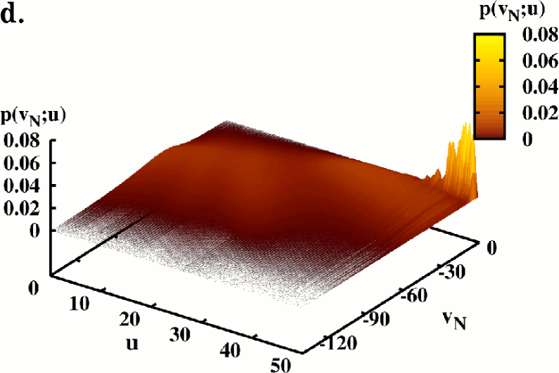
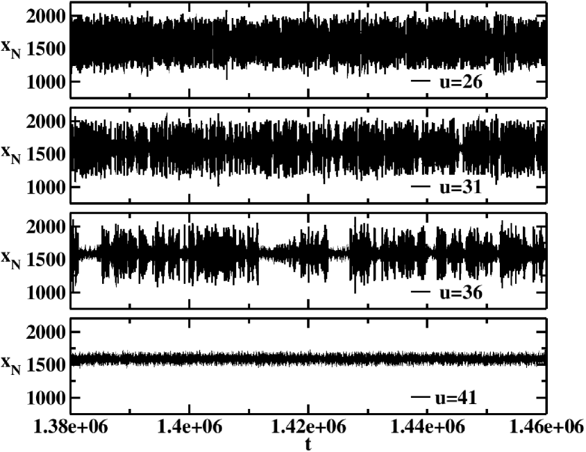
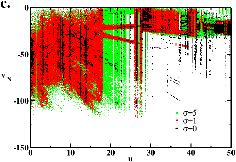
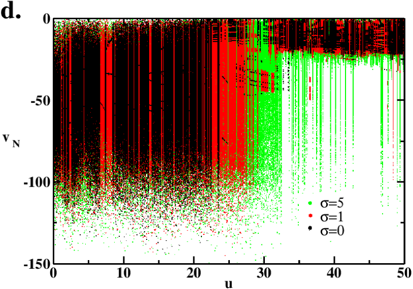
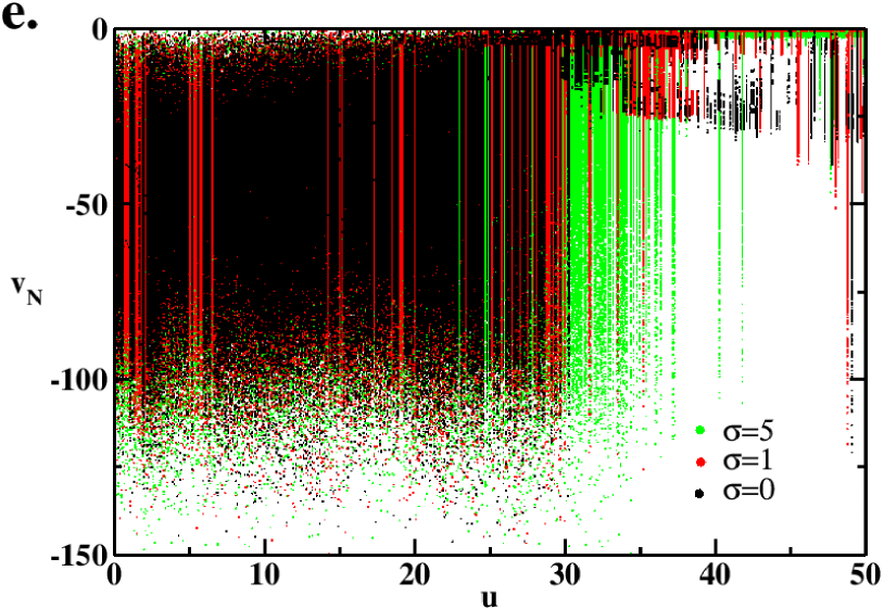
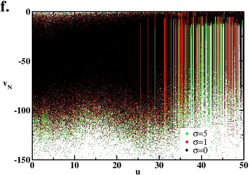
This observation can be explained through a quantitative change in the systems dynamics in the presence of noise. As we have seen before, the dynamics changes from chaotic to periodic or quasi-periodic via an intermittent behavior. For , intermittency occurs even without noise. This is nicely illustrated by the graphs for different values in Fig. 20. The intermittency found in the transition interval explains why the sharp phase transition-like behavior disappears for larger systems. As the disorder parameter measures the fluctuations of the chain length, in the intermittent region smaller disorder parameters will be observed. Fig. 20 indicates that larger and larger periodic or quasi-periodic time intervals appear at increased chain velocities. Therefore, the sharp transition becomes smoother. For increasing system sizes, the previously observed noise induced phase transition-like behavior becomes also less evident, as illustrated by Fig. 21, for driving velocities above the transition region.
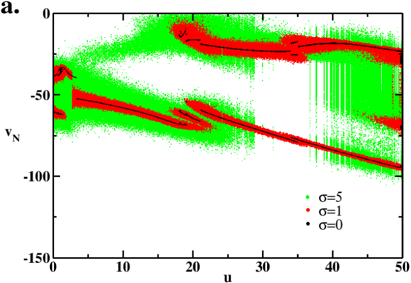
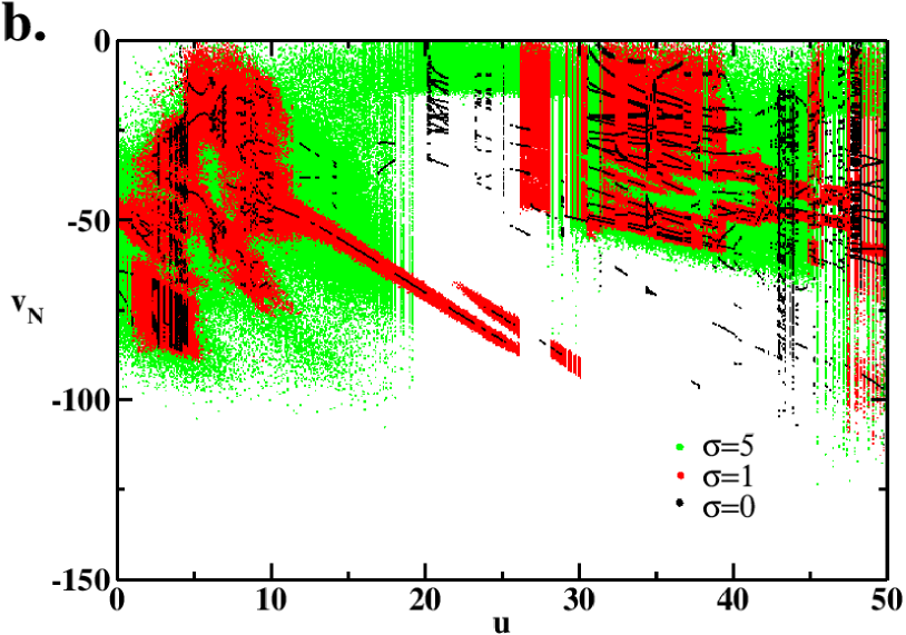
Bifurcation diagrams generated for different system sizes are shown in Fig. 22. These results augment those obtained from disorder parameter. They indicate that for , the system has only periodic or quasi-periodic attractors. The behavior of the disorder parameter does not suggest any phase transition-like behavior here. Dominant chaotic regimes appear for . As the size of the system is increased, the number of periodic windows decreases, and the transition region is enlarged. Also, for larger systems the effect of noise is less pronounced.
VI Discussion
The dynamics of a simple spring-block chain placed on a running conveyor belt was investigated both by simple experiments and through computer simulations. Despite its simplicity, the dynamics of the system proved to be quite complex exhibiting- chaotic, periodic or quasi-periodic behavior as a function of the conveyor belt’s velocity and the amount of noise in the friction forces. The experiments and computer simulations indicate that the transition from chaotic to periodic or quasi-periodic dynamics is typically realized through an intermittent chaotic state.
In the chaotic regime, the avalanche-size distribution function shows a scale-free nature, indicating also the presence of SOC, along with a type of stochasticity in the chain length. Another aspect of the systems complexity is the diversity of the possible dynamical states reflected by the convoluted graph of the bifurcation diagram, and a phase transition-like behavior in the disorder parameter. The presence of noise adds to this picture fascinating phenomena, like noise induced chaos, noise induced intermittency and noise induced phase transition.
Interestingly, the computer simulations suggest that the maximal complexity of the dynamical states is achieved for a relatively small number of blocks in the vicinity of for . For there is practically no chaos in the system. With the observed transition is the sharpest one, and for it becomes smoother in a somewhat counter intuitive way. It is remarkable that this collective behavior finds its explanation in terms of dynamical system properties.
Finally we would like to draw the attention to the fact that in several recent experimental studies Mudrock2011 ; Roth2012 performed on metallic alloys, it has been observed that just before the onset of the plastic instability the local strain rate as a function of the corresponding force response shows a multi periodic behavior. This is somehow similar with the graphs shown in Fig. 11. This observation brings us back to the possibility of modeling the Portevin- Le Chatelier effect with a spring-block system Lebyodkin1995 . Indeed, if the plastic deformation is macroscopically uniform in the absence of plastic instability, one can assume that it is governed by only a small number of collective degrees of freedom, similarly with the dynamics of the spring-block chain considered here. In such view the studied model and the obtained results can gain interest in the field of material science as well.
Acknowledgements.
The useful comments and advices of Gábor Drótos and Gábor Csernák are acknowledged. The work of FJ-SZ and ZN is supported from the IDEAS research grant: PN-II-ID-PCE-2011-3-0348. The work of BS was subsidized by ”Collegium Talentum” of Hungary and by the Excellence Bursary of BBU. The research of BS and TT is conducted in the framework of TÁMOP 4.2.4.A/1-11-1-2012-0001 ’National Excellence Program’ and OTKA NK100296. Financial support for this program is provided jointly by the Hungarian State, the European Union and the European Social Fund.*
Appendix A Numerical method
We briefly describe here the method used to integrate the Newton-equations (1) and to handle the discontinuous stick-slip dynamics of the blocks. If a block is stuck to the conveyor belt, then it will move together with it at constant velocity . Therefore, the position of the th block relative to the ground is calculated with the simple
| (5) |
equation. When a block is slipping relative to the belt, the basic Verlet method
| (6) |
is used to update its position. As can be seen, this is a third order method, which can be extended also to the velocity space Lazar2010 as:
| (7) |
The instance when the th block sticks to the belt is found when the relative velocity changes its sign, while the instance when the block starts to slip is defined by the sign change of . A more complicated stochastic numerical method was also developed to handle the stick-slip dynamics, but was found not to significantly alter the presented results.
References
- (1) P. Bak, C. Tang, and K. Wiesenfeld, Phys. Rev. Lett. 59, 381 (1987)
- (2) P. Bak, C. Tang, and K. Wiesenfeld, Phys. Rev. A 38, 364 (1988)
- (3) P. Bak and C. Tang, J. Geophys. Res-Solid 94, 15635 (1989)
- (4) J. M. Carlson and J. S. Langer, Phys. Rev. Lett. 62, 2632 (1989)
- (5) Z. Neda, F. Jarai-Szabo, E. Kaptalan, and R. Mahnke, Control Engineering And Applied Informatics 11, 3 (2009)
- (6) M. A. Lebyodkin, Y. Brechet, Y. Estrin, and L. P. Kubin, Phys. Rev. Lett. 74, 4758 (1995)
- (7) J. V. Andersen, Y. Brechet, and H. J. Jensen, Europhys. Lett. 26, 13 (1994)
- (8) J. V. Andersen, Phys. Rev. B 49, 9981 (1994)
- (9) K. T. Leung and Z. Neda, Phys. Rev. Lett. 85, 662 (2000)
- (10) F. Járai-Szabó, S. Astilean, and Z. Néda, Chem. Phys. Lett. 408, 241 (2005)
- (11) F. Jarai-Szabo, E.-A. Horvat, R. Vajtai, and Z. Neda, Chem. Phys. Lett. 511, 378 (2011)
- (12) K. Kovacs, Y. Brechet, and Z. Neda, Model. Simul. Mater. Sc. 13, 1341 (2005)
- (13) E.-A. Horvat, F. Jarai-Szabo, Y. Brechet, and Z. Neda, Cent. Eur. J. Phys. 10, 926 (2012)
- (14) F. Jarai-Szabo, B. Sandor, and Z. Neda, Cent. Eur. J. Phys. 9, 1002 (2011)
- (15) F. Járai-Szabó and Z. Néda, Physica A 391, 5727 (2012)
- (16) R. Burridge and L. Knopoff, Bull. Seism. Soc. Am 57, 341 (1967)
- (17) B. Gutenberg and C. Richter, Ann. Geofis. 9, 1 (1956)
- (18) H. Kawamura, T. Hatano, N. Kato, S. Biswas, and B. K. Chakrabarti, Rev. Mod. Phys. 84, 839 (May 2012)
- (19) J. M. Carlson and J. S. Langer, Phys. Rev. A 40, 6470 (1989)
- (20) H. J. Xu and L. Knopoff, Phys. Rev. E 50, 3577 (1994)
- (21) V. B. Ryabov and H. M. Ito, Phys. Rev. E 52, 6101 (1995)
- (22) M. de Sousa Vieira, Phys. Rev. Lett. 82, 201 (1999)
- (23) J. Szkutnik, B. Kawecka-Magiera, and K. Kulakowski, in Transient Processes in Tribology, Tribology Series, Vol. 43 (2004) pp. 529–536
- (24) B. A. Erickson, B. Birnir, and D. Lavallee, Geophys. J. Int. 187, 178 (2011)
- (25) M. de Sousa Vieira, G. L. Vasconcelos, and S. R. Nagel, Phys. Rev. E 47, R2221 (1993)
- (26) M. de Sousa Vieira, Phys. Rev. A 46, 6288 (1992)
- (27) M. de Sousa Vieira and H. J. Herrmann, Phys. Rev. E 49, 4534 (1994)
- (28) T. Baumberger, C. Caroli, B. Perrin, and O. Ronsin, Phys. Rev. E 51, 4005 (1995)
- (29) G. L. Vasconcelos, Phys. Rev. Lett. 76, 4865 (1996)
- (30) F.-J. Elmer, J. Phys. A - Math. Gen. 30, 6057 (1997)
- (31) H. Sakaguchi, J. Phys. Soc. Jpn. 72, 69 (2003)
- (32) A. Johansen, P. Dimon, C. Ellegaard, J. S. Larsen, and H. H. Rugh, Phys. Rev. E 48, 4779 (1993)
- (33) M. de Sousa Vieira and A. J. Lichtenberg, Phys. Rev. E 53, 1441 (1996)
- (34) C. V. Chianca, J. S. Sa Martins, and P. M. C. de Oliveira, Eur. Phys. J. B 68, 549 (2009)
- (35) M. de Sousa Vieira, Phys. Lett. A 198, 407 (1995)
- (36) J. Szkutnik and K. Kulakowski, Int. J. Mod. Phys. C 13, 41 (2002)
- (37) B. Erickson, B. Birnir, and D. Lavallee, Nonlinear Proc. Geoph. 15, 1 (2008)
- (38) U. Galvanetto, Physics Letters A 248, 57 (1998)
- (39) U. Galvanetto, Physics Letters A 293, 251 (2002)
- (40) F. P. Bowden and D. Tabor, Friction and Lubrication (Oxford University Press, 1954)
- (41) T. Tel, Y.-C. Lai, and M. Gruiz, Int. J. Bifurcat. Chaos 18, 509 (2008)
- (42) T. Tél and M. Gruiz, Chaotic Dynamics (Cambridge University Press, 2006)
- (43) Y.-C. Lai and T. Tel, Transient Chaos (Springer, New-York, 2011)
- (44) M. Iansiti, Q. Hu, R. M. Westervelt, and M. Tinkham, Phys. Rev. Lett. 55, 746 (1985)
- (45) H. Herzel, W. Ebeling, and T. Schulmeister, Z. Naturforsch. A 42, 136 (1987)
- (46) A. R. Bulsara, W. C. Schieve, and E. W. Jacobs, Phys. Rev. A 41, 668 (1990)
- (47) A. Hamm, T. Tel, and R. Graham, Phys. Lett. A 185, 313 (1994)
- (48) Z. I. Lázár, Studia UBB Physica 55, 95 (2010)
- (49) R. N. Mudrock, M. A. Lebyodkin, P. Kurath, A. J. Beaudoin and T. A. Lebedkina, Scripta Mater. 65, 1093 (2011)
- (50) A. Roth, T. A. Lebedkina, and M. A. Lebyodkin, Mat. Sci. Eng. A 539, 280 (2012)