Characterization of production sets through individual returns-to-scale: a non parametric specification and an illustration with the U.S industries
Abstract
This paper proposes to estimate the returns-to-scale of production sets by considering the individual return of each observed firm through the notion of -returns to scale assumption. Along this line, the global technology is then constructed as the intersection of all the individual technologies. Hence, an axiomatic foundation is proposed to present the notion of -returns to scale. This new characterization of the returns-to-scale encompasses the definition of -returns to scale, as a special case as well as the standard non-increasing and non-decreasing returns-to-scale models. A non-parametric procedure based upon the goodness of fit approach is proposed to assess these individual returns-to-scale. To illustrate this notion of -returns to scale assumption, an empirical illustration is provided based upon a dataset involving 63 industries constituting the whole American economy over the period 1987-2018.
JEL: D24
Keywords: Returns to Scale, Increasing Returns to Scale, Efficiency, Minimum extrapolation, Data Envelopment Analysis.
1 Introduction
As an important feature of the production process, returns-to-scale provide information about the production technology such as marginal products and linearity of the process (Podinovski et al., 2016; Podinovski, 2022; Sahoo and Tone, 2013; Tone and Sahoo, 2003). In addition, returns-to-scale (RTS) are also related to the notion of economies of scale and of scope that are involved in performance measurement.
Considering the importance of RTS and based upon the notion of homogeneous multi-output technologies (Lau, 1978; Färe and Mitchell, 1993), Boussemart et al. (2009, 2010) introduce an approach allowing to characterize either strictly increasing or strictly decreasing RTS alongside the traditional RTS (non increasing, non decreasing, constant), in multi-output technologies. This approach is named the -returns to scale model. It provides more theoretical foundation than the traditional data envelopment analysis (DEA) models (Charnes et al., 1978; Banker et al.,1984) by considering all RTS involved in the production process. Indeed, the traditional DEA models just allow either constant or variable RTS such as variable RTS only encompasses non increasing, non decreasing and constant RTS. In addition, the -returns to scale model allows involving zero data within the production set, and also proposes to model production sets with strictly increasing RTS, as defined in the literature.
The -returns to scale model (Boussemart et al., 2009) is defined from a global standpoint (i.e. by considering all the observation as a whole). This means that which represents the RTS, is a singleton that is applicable to the whole production set. The estimated -returns to scale is optimal when it characterizes the production frontier that minimizes the inefficiency of the set of observations. As is a singleton representing only one RTS that characterizes the production frontier, the -returns to scale model does not consider the local structure of RTS that individually applies to each observation. To overcome this issue, this paper extends the -returns to scale model to a more general case through the -returns to scale model. Indeed, the -returns to scale model defines which represents the RTS of the production set as a subset of the non negative real line that may contain an infinity of elements. Hence, can encompasses all kind of RTS. The -returns to scale model is more general since it encompasses as special cases the -returns to scale model (i.e. if is a singleton then it reduces to ) as well as variable, non increasing and non decreasing RTS models. Moreover, the -returns to scale model has as limits in zero and infinity, the input and the output ray disposabilities, respectively. As the -returns to scale model takes into account the local structure of RTS then, the production set can be either convex or non convex. Hence, the production set is not a priori assumed to be convex as in traditional economic literature. Relaxing the convexity property is of particular interest mainly by allowing to take account strictly increasing marginal products as well as possible non linearity in the production process. is first defined through an individual point of view. This means that each observation is associated to its individual -returns to scale that corresponds to a local RTS of the global production technology. Once the individual -returns to scale determined, the global -returns to scale can be deduced as the union of the individual . This global -returns to scale characterize the overall technology. Notice that the optimal is the RTS that minimize the inefficiency of firms. The global production set that involves all the observations is then the intersection of each individual production technology with respect to . This means that allows to introduce a new class of production sets as they are defined regarding the RTS.
Boussemart et al. (2009, 2010) provide a non parametric approach to implement the -returns to scale model. Indeed, they defined through the constant elasticity of substitution (CES) - constant elasticity of transformation (CET) production technology (Färe et al., 1988). This first approach exogenously assesses since the efficiency of firms are evaluated with respect to an imposed set of possible values of . Leleu et al. (2012) applied this exogenous procedure by using a DEA approach, to provide an empirical analysis of the optimal productive size of hospitals in intensive care units. More recently, Boussemart et al. (2019) propose to consider as an endogenous variable. They propose to assess through a minimum extrapolation principle and the Free Disposal Hull (FDH) model (Deprins et al., 1984; Tulkens, 1993). This approach allows to evaluate the optimal RTS through a non parametric scheme and a linear program. In this line, this paper proposes to assess the -returns to scale model following the approach provided in Boussemart et al. (2019).
To summarize, the main objective of this paper is threefold. (i) An axiomatic foundation of a generalized RTS is defined through the -returns to scale model. It allows to characterize a production technology minimizing the inefficiency of firms. (ii) A new class of production sets is introduced regarding the -returns to scale model. (iii) A non parametric procedure is proposed to assess the -returns to scale through linear programs.
The remainder of this paper is structured as follows. Section 2 presents the backgrounds on the production technology, efficiency measurement and the -returns to scale model. The notion of -returns to scale and its connection with standard models are presented in section 3. Section 4 proposes a general procedure to estimate the -returns to scale based upon the individual -returns to scale and from an input oriented standpoint. Section 5 provides an empirical illustration by the means of a dataset about 63 industries constituting the whole American economy such that the data is composed with one output and three inputs and covers the period 1987-2018. Section 6 resumes and concludes.
2 Backgrounds
This section aims to introduce the notation and the theoretical basis used throughout this paper. Subsection 2.1 defines the production technology as well as the efficiency measure. Subsection 2.2 describes the -returns to scale model.
2.1 Production technology: assumptions and key concepts
The production technology is the process transforming an input vector composed of components into an output vector containing elements, and defined by:
| (2.1) |
The technology satisfies the following regular axioms: () no free lunch and inaction; () infinite outputs cannot be obtained from a finite input vector; () the production set is closed; () the inputs and outputs are freely disposable. Remark that the technology is convex neutral meaning that the convexity of the production set is not a priori assumed. Also notice that when setting empirical analyses, the production sets may not satisfy all the axioms .
The efficiency measure of production units can be evaluated through distance functions that assess the distance between the observation and the efficient frontier. One of the most used efficiency measure is the Farrell efficiency measure (Debreu, 1951; Farrell, 1957) that can be either input oriented or output oriented. For any the input Farrell measure provides the maximum radial contraction of the input vector for a given level of outputs and is defined as . In the same vein, the output Farrell measure gives the maximum radial expansion of the output vector for a given amount of inputs and is defined as . Remark that the input Farrell measure takes value between 1 and 0. If the observation does not belong to the production set then, both input and output Farrell measures are indeterminate . Besides, if the production unit is efficient i.e. belongs to the efficient frontier then, the input and/or the output Farrell measure is equal to 1.
Following the proposed definition of Färe and Mitchell (1993), a production technology is homogeneous of degree if for any and any , Obviously, this notion of homogeneity of degree is connected to the notion of returns-to-scale. Indeed, constant returns-to-scale (CRS) corresponds to while strictly increasing returns (IRS) correspond to and strictly decreasing returns (DRS) correspond to . Boussemart et al. (2009, 2010) termed this property of the technology as “-returns to scale”. Boussemart et al. (2010) show that under such an assumption, some existing measures (Farrell output measure, hyperbolic efficiency measure of Färe et al., 1985; proportional distance function of Briec, 1997) can be related in closed form under an -returns to scale assumption.
2.2 -returns to scale : non-parametric approach and extrapolation principle
In the line of Boussemart et al. (2009), Boussemart et al. (2019) propose a non-parametric approach to estimate the best returns-to-scale allowing to maximize the global efficiency of the whole considered production set. To do so, they consider a constant elasticity of substitution - constant elasticity of transformation (CES-CET) production set (Färe et al., 1988) and apply the minimum extrapolation principle to a Free Disposal Hull (FDH - Deprins et al., 1984) type model by means of input and output-oriented Farrell efficiency measures. For any firm belonging to the set of firms , the global technology is the union of each individual technology with , where:
| (2.2) | ||||
| and | (2.3) |
Remark that the global technology is the production set including all the observations whereas the individual technology is a production possibility set derived from and related to the observation . Boussemart et al. (2009) prove that satisfies -. The efficiency of each production unit is then assessed with respect to each individual technology . In such case, for , the efficiency measures and are respectively the input and the output Farrell measure of the observation with respect to . Boussemart et al. (2009, 2010) demonstrate that for ,
| (2.4) | ||||
| and | (2.5) |
By definition, since the observation is evaluated with respect to its own individual technology . Remark that stands for the -th component of the input vector of firm . Also, note that and where and are the number of elements in input and output vectors, respectively.
Notice that the following convention is adopted: for any , if and , then .
Figure 1 describes the individual production sets for each observation. Notice that the represented production sets are non convex resulting in illustrating efficient frontiers related to strictly increasing RTS for , , and .
3 On some extended notions of -returns to scale
This section aims to propose the axiomatic foundation of the generalized -returns to scale model. Subsection 3.1 presents its definition while Subsection 3.2. displays the connection with this new RTS model and the traditional ones.
3.1 -returns to scale: definition and some basic properties
Boussemart et al. (2019) show that empirical procedures may provide infinite () and null () returns-to-scale. Formally, a production set satisfies a -returns to scale assumption if for any scalar and if the production unit belongs to then, also belongs to . This definition is obtained from the standard definition setting . Note that, equivalently, a production set satisfies a -returns to scale assumption if for all , an observation belonging to means that is also part of Along this line, a production set satisfies an -returns to scale assumption, if for any and if the production unit then, .
The -returns to scale assumption and -returns to scale assumption are limit cases of the -returns to scale assumption when and . Surprisingly, -returns to scale assumption and -returns to scale assumption correspond to the input and output ray disposability (T4) assumption, respectively.
Figure 2 illustrates the -returns to scale (figure on the left) and -returns to scale (figure on the right) assumptions. Obviously, the figure on the left illustrate the input strong disposability since for , the same level of output () is provided by a higher level of input (). Besides, the figure on the right presents the output strong disposability, since for , the same level of input () can produce a lower level of outputs (). Note that -returns to scale may be not compatible with the no free lunch axiom () for any positive output. In addition -returns to scale do not hold if holds.
In the following the notion of -returns to scale is extended.
Definition 3.1.
Let be a subset of . We say that a technology satisfies a -returns to scale assumption if there exists a family of production sets where for any , satisfies an -returns to scale assumption and such that:
| (3.1) |
Notice that there is no specific restriction on except that it is a set of positive real numbers and may be finite. This definition has the advantage to give information about the local nature of the technology and to propose a more general class of technologies involving some special local returns-to-scale. Indeed, is a singleton representing an individual returns-to-scale associated to a given observation allowing to minimize its inefficiency whereas combines any individual returns-to-scale aiming to provide the global returns-to-scale and the characterization of the overall production set. An expanded explanation of this definition is displayed in Section 4 (Proposition 4.1).
In Figure 3, the production set satisfies a -returns to scale assumption. However it does not satisfy an -returns to scale assumption neither an -returns to scale assumption, if they are considered separately as singletons.
Remark that larger is the collection , larger is the potential number of technologies satisfying a -returns to scale assumption. Indeed, if is large then there is more class of technologies that is embedded within the technology satisfying a -returns to scale assumption.
We consider the following examples.
Example 3.2.
Suppose that and with . By construction,
Let us denote and . We have . Clearly, satisfies a -returns to scale assumption and satisfies a -returns to scale assumption. Therefore satisfies a -returns to scale assumption. Also if it also satisfies a -returns to scale assumption. only satisfies .
Example 3.3.
Suppose that and with . By construction
Let us denote and . We have . Clearly, satisfies a -returns to scale assumption and satisfies a -returns to scale assumption. Therefore satisfies a -returns to scale assumption. This situation might occur when the available input quantity is limited. only satisfies . Another symmetrical case is given by the production set . Clearly, satisfies a -returns to scale assumption. This type of situation might arise when a technology requires the production of a minimal amount of output.
Example 3.4.
Suppose that and with . Let us denote , and . We have . Clearly, satisfies a -returns to scale assumption, a constant returns to scale assumption and satisfies a -returns to scale assumption. Therefore satisfies a -returns to scale assumption.
Notice that although the production process satisfies some standard axioms, there is no guarantee that the smallest technology satisfying an -returns to scale assumption and containing the production process, obeys these axioms. For example the conical hull of a closed set may not be closed and might be violated. Also, in the case where , no longer holds true.
Remark that a production set satisfies a minimal -returns to scale assumption if satisfies a -returns to scale assumption and if for all
| (3.2) |
This means that the identified is the minimal returns-to-scale allowing to characterize the entire production set.
Example 3.5.
Suppose that and with . Let us denote , and . We have . Clearly, satisfies a -returns to scale assumption when and satisfy a constant returns to scale and a -returns to scale assumptions, respectively. Therefore, satisfies a -returns to scale assumption. However, is not an active constraint. Thus, we also have . Hence, is -minimal but not -minimal.
Let us define, for all , the -conical hull of any subset of as:
| (3.3) |
Notice that if , then Obviously, when , we retrieve the standard concept of conical hull.
We say that the returns-to-scale of a production set are -bounded if is contained by at least one production set satisfying and an assumption of -returns to scale. In addition is -bounded if is -bounded for all . This implies that the RTS of a production set belong to if is contained by at least one technology satisfying a -returns to scale assumption. For example in Figure 3, is obviously -bounded. Nonetheless, is not -bounded. Remark that this statement do not postulate any assumption on .
The next statement show that if the RTS of a production set are -bounded, then there exists a smallest technology containing it and satisfying a -returns to scale assumption.
Lemma 3.6.
Let be a production set and suppose that the returns to scale of are -bounded, for some . Let us denote, . Then, is the smallest technology satisfying an assumption of -returns to scale that contains .
See proof in Appendix 2.
Figure 4 illustrates Lemma 3.6 where is contained by a technology satisfying an -RTS assumption. Depending on the value of , can be either convex or non-convex. With , the production technology is a convex set demonstrating a strictly decreasing RTS. Besides, with , the technology is a non-convex set showing a strictly increasing RTS.
The result in Lemma 3.6 extends the construction proposed in Section 2.2 to the case of a general technology. In particular, note that for each production vector we have where . Also notice that we do exclude the situation where Remark that a specific situation arises when a technology satisfies a -returns to scale assumption and when we consider its -extrapolation with
Lemma 3.7.
Suppose that is a production set satisfying an -returns to scale assumption. Suppose that , is a positive real number with . Then, either fails to satisfy or , for all
See proof in Appendix 2.
The next result is an immediate consequence of Lemma 3.6.
Proposition 3.8.
Let be a production set and suppose that the returns-to-scale of are -bounded, where is a subset of . For all , let us denote . Then,
is the smallest production set satisfying a -returns to scale assumption that contains , i.e. if and satisfies a -returns to scale assumption, then .
See proof in Appendix 2.
Figure 5 illustrates Proposition 3.8. This figure is the combination of the two possibilities in Figure 4 where can be contained by either with or where . Resulting from Proposition 3.8, .
The existence of a minimal intersecting technology allows to state that it is always possible to associate any -bounded production set with its minimal extrapolation. For any production set , the production process is a -minimal extrapolation of if is the smallest production set satisfying a -returns to scale assumption that contains . It follows that if satisfies a -returns to scale assumption, then:
| (3.4) |
Proposition 3.9.
Let and be two subsets of . Suppose that is a -bounded and -bounded production set. Then the and minimum extrapolation of satisfy the following properties:
-
if ,
-
,
-
if .
See proof in Appendix 2.
In the following, we show that if contains some , then the -minimal extrapolation of satisfies , and independently of . This condition avoids the shortcomings of the cases and An additional condition is required for the closedness of
Proposition 3.9 shows that the larger is the set and the more vague is the global returns-to-scale structure of the production set. Remark that if is a singleton then the technology satisfies an -returns to scale assumption. Doing so, we introduce an alternative formulation of the notion of -returns to scale.
A production set satisfies a :
-
(i)
right- returns to scale assumption if for all ,
(3.5) -
(ii)
left- returns to scale assumption if for all
(3.6)
Remark that when then, satisfies a left- returns to scale assumption if, for all , The next proposition connects the alternative formulation of -returns to scale with the notion of -returns to scale.
Proposition 3.10.
Let be a closed interval of . Let us denote and . Suppose that satisfies a -returns to scale assumption and that for each , satisfies . Then, satisfies a right- returns to scale assumption and a left- returns to scale assumption.
See proof in Appendix 2.
The key intuition is that, when is an interval, the returns-to-scale are characterized by its lower and upper bounds. Notice that if a production set satisfies a right- returns to scale assumption then,
for all and all , we have . Besides, if satisfies a left- returns to scale assumption then
for all and all , we have .
Figures 7 and 7 describe the notions of right- and left- RTS. Specifically, Figure 7 illustrates these notions within Proposition 3.10 framework by considering right- and left- RTS assumptions in general cases. Besides, Figure 7 illustrates the limit cases of the left- RTS assumption with and of the right- RTS assumption where .
3.2 From -returns to scale to Non Increasing, Non Decreasing and Variable returns-to-scale
In this subsection, we show that traditional convex and non-convex models involving a returns-to-scale assumption, follow a special case of the -returns to scale assumption.
For a given set of production units , each individual production possibility set is based upon (i) a single production unit with , (ii) the strong disposability assumption and (iii) some hypotheses of returns-to-scale. Notice that some of these returns-to-scale assumptions are namely Constant (CRS), Non Increasing (NIRS), Non Decreasing (NDRS) and Variable (VRS) returns-to-scale. Starting from the notation introduced in Eq.(2.3), let us denote the individual production set as:
| (3.7) |
where , with: ;
;
;
Remark that denotes the returns-to-scale assumption whereas means that .
Union and convex union of these individual production possibility sets yield non convex (NC) technologies on the one hand and traditional convex (C) possibility sets on the other hand, as follows:
| (3.8) |
where is the convex hull operator.
Regarding the convex case, we retrieve the standard DEA model initiated by Charnes et al. (1978) and Banker et al. (1984). Besides, the non-convex case provides the model proposed by Deprins et al. (1984) and Tulkens (1993).
Additionally to the returns-to-scale assumption, convexity constraints can be added to the characterization of the production technology. Consider the following notations:
| (3.9) |
An unified algebraic representation of convex and non convex technologies under different returns-to-scale assumptions for a sample of observations is as follows (Briec et al., 2004):
| (3.10) |
where . Notice that () is an activity vector related to either a convexity () or a non convexity
() constraint. Moreover, () is a scaling parameter allowing the particular scaling of
all observations involved in the technology. This scaling parameter is positive and smaller than or equal to 1 under , larger than or equal to 1 under , fixed at unity under and, free under assumptions.
However, there is a shortcoming with this formalism. It does not include and therefore, does not take into account inaction in the and cases. To circumvent this problem we slightly modify the above definition (Eq. 3.10) by introducing the sets
| (3.11) |
Clearly if either or then .
The next statement is an immediate consequence of our earlier results and shows that the standard DEA convex models satisfy special cases of the -returns to scale assumption.
Proposition 3.11.
For any subset of and any we have the following properties:
-
If then and satisfies a -returns to scale assumption.
-
If then and satisfies a -returns to scale assumption.
-
If then satisfies a -returns to scale assumption.
-
If then and satisfies a -returns to scale assumption.
See proof in Appendix 2.
Along this line, the next proposition shows that , and production technologies can be derived from an extrapolation of the -returns to scale assumption with the model.
Proposition 3.12.
For any subset of and any we have:
-
;
-
;
-
.
Figure 8 illustrates statements and of Proposition 3.12 with for NIRS and NDRS assumptions. Remark that the production frontiers are piecewise linear showing the characteristics of the RTS assumptions.
Figure 9 illustrates statements and of Proposition 3.11 with . The production frontiers are piecewise linear and highlight the specificity of the CRS and the VRS assumptions.
Since the model satisfies a -returns to scale assumption, it is both the more general and the less informative about the returns-to-scale structure of the production set. Interestingly, union and intersection on allow to relate the , and models. However, these operations are intrinsically derived from the specific nature of the returns-to-scale. Note that although , satisfies a -returns to scale assumption. Conversely, although , satisfies a -returns to scale assumption (see Eq (3.7) and Proposition 3.11).
4 From individual -returns to scale to global -returns to scale assumption and technology
This section presents the minimum extrapolation principle that is used to define the production technology of the data set. Moreover, a procedure is proposed to assess the individual optimal value of under a generalized FDH technology and through an input-oriented model. This approach fully endogenizes the assessment of through linear programming. From these individual , the global optimal value of is derived allowing to characterize the returns-to-scale of the whole production set.
4.1 -Returns to scale and minimum Extrapolation
In this section, we introduce the principle of minimum extrapolation allowing to define the notion of rationalized technology.
The next proposition presents the minimum extrapolation principle for the individual technologies and their union .
Proposition 4.1.
For all and a data set ,
-
is the smallest technology containing that satisfies and an -returns to scale assumption.
-
is the smallest technology containing that satisfies and an -returns to scale assumption.
From Proposition 4.1, we can now introduce the lower, upper and minimal extrapolation technologies for each observation as follows:
-
(i)
The lower individual minimal extrapolation is denoted
(4.1) -
(ii)
The upper individual minimal extrapolation is defined as:
(4.2) -
(iii)
The individual minimal extrapolation is obtained from the union over :
(4.3)
Remark that for the sake of simplicity, we note and the -returns to scale and -returns to scale related to the observation .
The two first aforementioned assertions mean that the lower (i) and the upper (ii) individual minimal extrapolations are provided by the union of individual technologies subjected to respectively the lower () and the upper () bounds of . The next section introduces these notions of upper and lower bounds. The third statement means that the individual minimal extrapolation technology is the union of individual technologies and is -bounded.
Notice that and are obtained by replacing with respectively and in , such that :
| (4.4) | |||
| (4.5) |
From the individual scheme, we can deduce the global production possibility set as follows:
-
(iv)
The lower minimal extrapolation of the technology is then defined as:
(4.6) -
(v)
The upper minimal extrapolation of the technology is:
(4.7) -
(vi)
The global minimal extrapolation of the technology is similarly defined as:
(4.8)
Statements (iv)-(vi) mean that the global technology involving all units of the set of observations is the intersection of all individual minimal extrapolation technologies.
Proposition 4.2.
Let and let us denote . Then,
-
satisfies a -returns to scale assumption.
-
satisfies a right -returns to scale assumption and a left -returns to scale assumption, with
See proofs in Appendix 2.
Proposition 4.2 means that (i) the returns-to-scale of the global technology is the union of each individual which is an interval that reduces to if it is a singleton. This global returns-to-scale of the global technology is also (ii) upper and lower bounded by and , respectively.
In the following, we say that a technology -rationalizes the data set if is the smallest technology satisfying a -returns to scale assumption with .
Proposition 4.3.
Let and denote then, -rationalizes the data set .
See proof in Appendix 2.
4.2 The non parametric input oriented model
Through the input oriented model, we look for the individual optimal related to the observation for any and that minimizes the inefficiency of the observed unit. This individual optimal of is noted and shortened as . To do so, a goodness of fit index minimized by , is defined (Boussemart et al., 2019). Formally, the definition of the goodness of fit index is as follows:
| (4.9) |
The goodness of fit index allows to provide the global efficiency measure for each observation given the range of efficiency measures that are related to each of them with respect to the range of individual technologies. Indeed, each individual technology provides an efficiency measure for each observation. This means that for a set of firms, each firm has efficiency measures then, the goodness of fit index allows to identify the optimal efficiency score with respect to .
Basically, the key idea is to consider in a first step process the optimisation of
only regarding firm . However, for some , all the potential technologies satisfying an -returns to scale assumption should contain the set of all the
observed production units. Notice that we could equivalently consider an approach based upon the output oriented measure . This key intuition is depicted in the figure below.
Figure 10 illustrates the lower and the upper bounds of the individual RTS of the observation . Indeed, is not a singleton then the individual RTS is an interval provided by the union of any -returns to scale related to .
The following program allows to solve the optimization problem :
| (4.10) |
The logarithmic transformation yields:
| (4.11) |
Setting , , and , the program becomes:
| (4.12) |
and the associated linear program is:
| (4.14) |
This linear program has variables and constraints. Denote the set of solutions for the program . As then .
From , the derived individual technology related to the observation is then:
| (4.15) |
where is obtained by replacing with in as follows:
| (4.16) |
A numerical example is proposed in Appendix 2 to illustrate the above notions.
Suppose now that there is an infinity of solutions to Program . Since the optimisation program is linear, the solution set is closed and convex. Therefore, there is an interval denoted as which contains all the solutions. Let us denote the solution in of then, and are respectively solutions of the programs below:
| (4.18) |
| (4.20) |
Indeed, as then, and are obtained by maximizing and minimizing , respectively. This means that when the Program has an infinity of solutions then, the optimal returns-to-scale of the observation is not a singleton ( but rather an interval with a lower () and an upper () bounds.
Note that for all and all :
| (4.21) |
Remark that are assessed with respect to , and , respectively.
Recall that for all we have:
It follows that
| (4.22) | ||||
| (4.23) |
Therefore, it follows that for all , the input measure computed over the global technology is obtained from the efficiency scores evaluated on and .
It can be useful to compute the efficiency score of any production vectors. This is the case in super-efficiency models and also for measuring productivity. More importantly, this allows to characterize the production technology.
In the input oriented case, for all we have:
| (4.24) |
Since we have
| (4.25) | ||||
| (4.26) |
For a lower minimal extrapolation case:
| (4.27) |
In the case of the upper minimal extrapolation:
| (4.28) |
5 Empirical illustration: estimation of individual -returns to scale for the US industries
This analysis focuses on the evolution of individual -returns to scale for 63 US industries totalling the whole American economy over the period 1987-2018. In this perspective, the theoretical framework developed above is applied to annual underlying technologies retaining one output and three inputs. The production is measured by the gross output while the inputs are intermediate inputs, labour and capital services delivered by equipment, buildings, and intellectual property products.
5.1 Data description and estimation strategy
All basic data are estimated by the Bureau of Economic Analysis (BEA) through yearly production accounts established for each specific industry (http://www.bea.gov/). The decision making units (DMUs) are the 63 industries (Appendix 1, Table 1).
All output and intermediate quantity indexes are weighted by their respective value levels in 2012 to obtain the gross output expressed in constant US dollar 2012. Volumes of fixed capital consumption are approximated by the cost depreciations of the three types of capital services (also expressed in constant 2012 prices). Finally, full-time employees measure annual changes in labour quantity.
This empirical illustration aims to provide the optimal individual -returns to scale for each industry (or Decision Making Unit - DMU). To do so, we implement the input-oriented model introduced in Subsection 4.1. Indeed, we first estimate the optimal input oriented individual -returns to scale which is noted . This is the maximal that minimizes the inefficiency score (), for each DMU (program ). Once obtained, we apply programs () and (). These two programs allow to determine if there exists, for each DMU, an interval () having a lower () and an upper () bounds, and which contains . In such case, we established a procedure to characterize the returns to scale as follows. If the lower () bound is greater than 1, then the industry is characterized by increasing returns (IRS). On the other hand, if the upper () bound is lower than 1, then the industry is characterized by decreasing returns (DRS). In both cases, it is clear that the hypothesis of constant returns to scale (CRS) can be rejected. However, when the interval includes 1 then, we consider that the hypothesis of CRS cannot be rejected.
5.2 Results
The averages of -returns to scale per industry over the entire period indicates that a majority of sectors are characterized by IRS (26 out of 63). There are 15 industries under DRS and 21 industries for which the CRS hypothesis is not rejected. The existence of strictly IRS as optimal ones, indicates that the production set is locally non-convex and that the production process is non-linear for these industries. Moreover, these IRS imply that some efficient observations could have increasing marginal products as well as they could also face indivisibilities (Tone and Sahoo, 2003; Sahoo and Tone, 2013) in the production process.
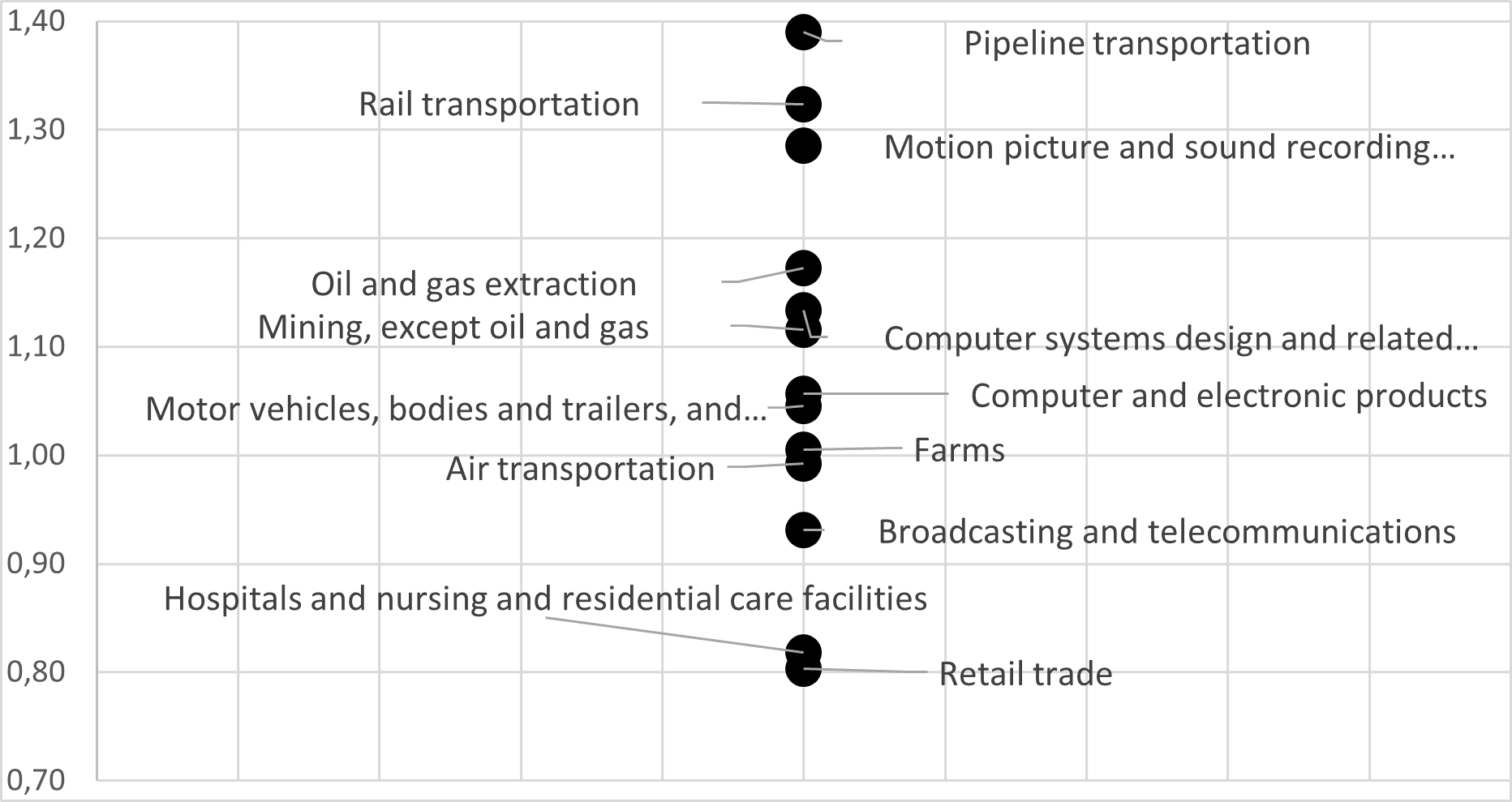
Figure 11 positions several emblematic industries with respect to their RTS. The activities concerning pipeline and rail transportations, motion picture, oil and gas extraction, mining, computer systems design are industries characterized by significantly IRS. The automotive sector and computers and electronics have slightly IRS. In contrast, hospitals and retail trade are clearly activities under DRS while broadcasting and telecommunications have slightly DRS. Finally, farms and air transport operate with CRS technologies.
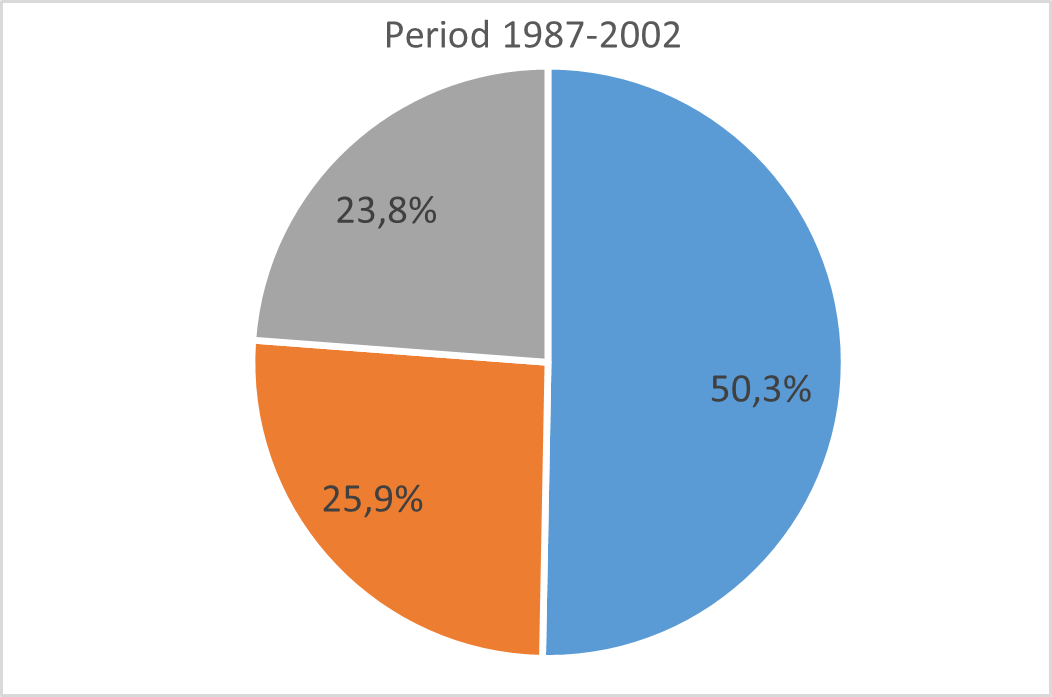
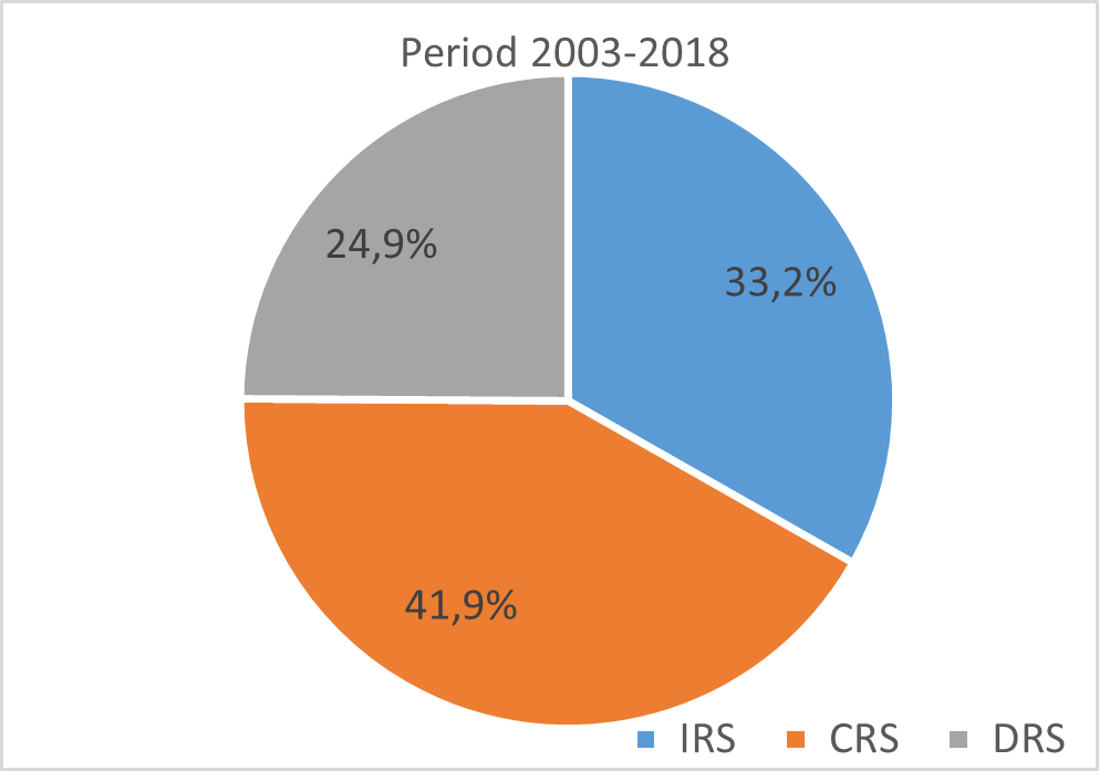
However, the annual changes of individual -RTS strongly this first result established in favour of the IRS which is calculated on a static average over the whole period. According to Figure 12, variations in -RTS per period show a structural evolution of the US economy towards more industrial activities characterized by CRS technologies. At the beginning of the period (1987-2002), more than 50% of sectors were characterized by IRS while those under CRS weighed only 24%. Over the more recent period (2003-2018), we observe a substantial decline in the share of IRS industries (33%) in favour of CRS sectors (42%). The share of DRS industries remains stable (26% to 25%).
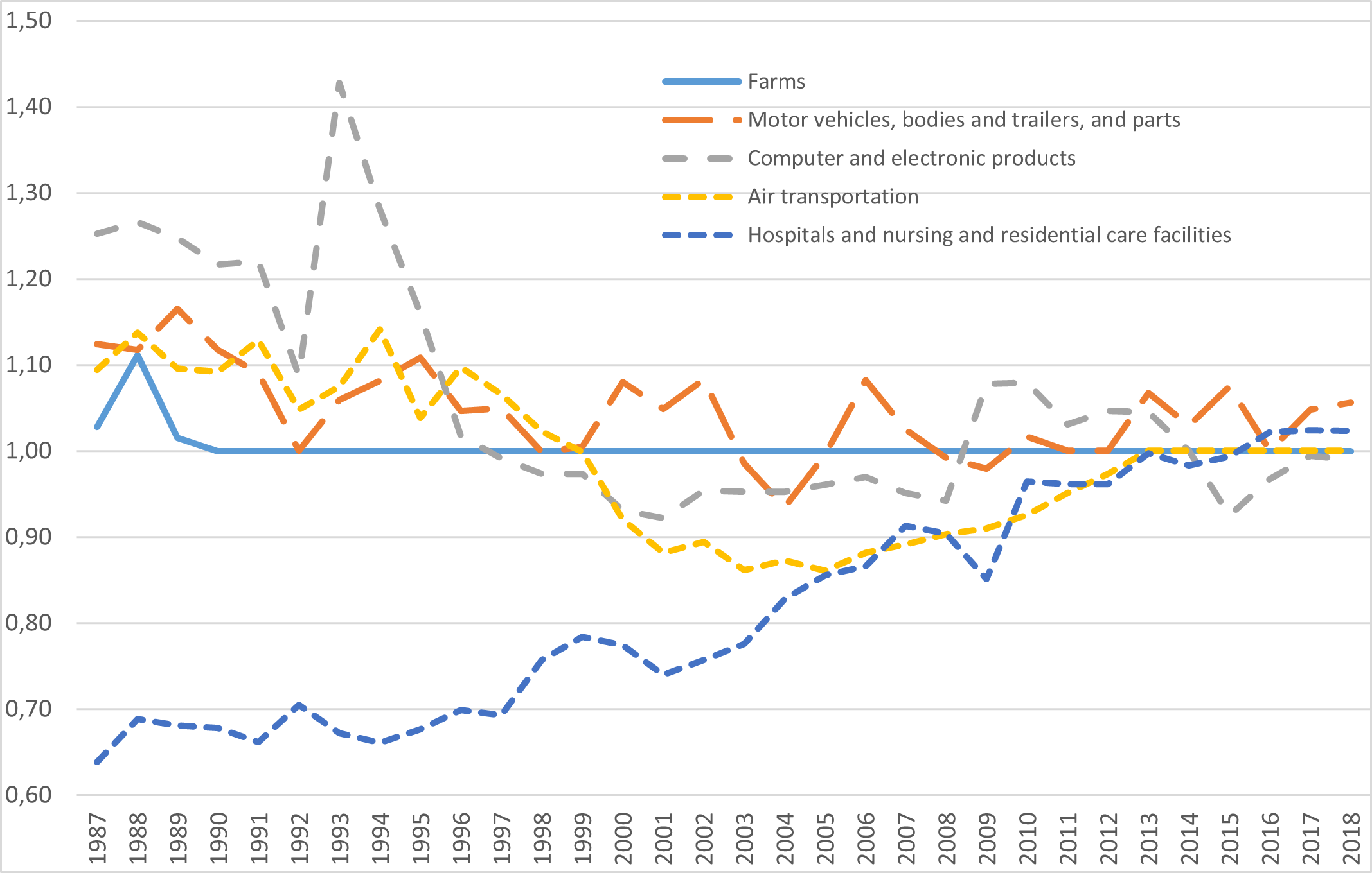
These results confirm those previously established by Boussemart et al. (2019) who had shown that estimates of the -RTS for the entire U.S. economy converged clearly towards unity. This indicates that the US economy has nearly converged to a CRS technology implying that industries tend to their most productive scale size (MPSS) improving their total factor productivity levels. Figure 13 illustrates this general finding with a few industry examples . The farms sector has maintained CRS throughout the period. The automotive sector’s returns to scale fluctuate slightly above unity with some trend convergence toward the CRS area. Air transportation experienced two distinct phases of convergence towards CRS: the first started from a situation characterized by IRS in 1987 to CRS in 1999. Then, after the shock of the early 2000s characterized by DRS, this industry again converged to the CRS zone. The computer and electronic products industry started the period with strongly IRS and finally reached CRS. Conversely, hospitals started from a strongly DRS technology and converged steadily towards a CRS technology.
The numerical results are displayed in Appendix 2.
6 Conclusion
This paper extends the notion of global -returns to scale model proposed by Boussemart et al. (2019). Indeed, the notion of -returns to scale is introduced as a subset of non-negative real line allowing to characterize the global technology. Indeed, an optimal “”-returns to scale is estimated for each observation constituting the production set. If is not a singleton then each observation is associated to an optimal individual -returns to scale which is an interval containing any optimal individual . Doing so, the local structure of returns-to-scale is considered such that the production possibility set can take into account strictly increasing and decreasing returns-to-scale. These particular returns are not often defined in standard models and hence some features of the production process may be neglected such as non linearity. Thereby, the global production possibility set can locally be non-convex. A non-parametric general procedure is provided to estimate the individual -returns to scale, from an input oriented standpoint. Each optimal individual -returns to scale may have an upper and a lower bounds as well as it can be a singleton. Along this line, the global technology is considered as an intersection of all individual production processes such that each individual returns-to-scale contributes to define the global -returns to scale of the global technology. Hence, the introduction of -returns to scale assumption allows to present a new class of production sets allowing to consider any kind of RTS.
These results are illustrated through a dataset composed of 63 industries constituting the whole American economy and which covers 32 years. The empirical results show that the -returns to scale model allows to identify strictly increasing and decreasing individual returns-to-scale. However, the global technology satisfies a variable returns-to-scale including strictly increasing and decreasing returns-to-scale contrary to standard DEA models. The general procedure proposed in this paper has been presented through an input orientation nonetheless, it is always possible to implement this minimal extrapolation principle from an output oriented standpoint. Also remark that it could be of interest to take account for noise in the efficiency assessment following the approach proposed by Simar and Zelenyuk (2011).
References
- [1] Banker R., Charnes A., Cooper W. (1984), Some Models for Estimating Technical and Scale Inefficiencies in Data Envelopment Analysis, Management Science, 30(9): 1078–1092.
- [2] Banker R. D., Maindiratta A. (1986), Piecewise Loglinear Estimation of Efficient Production Surfaces, Management Science, 32(1): 126-135.
- [3] Boussemart J-P., Briec W., Peypoch N., Tavera C. (2009), -Returns to scale and multi-output production technologies, European Journal of Operational Research,19: 332-339.
- [4] Boussemart J-P., Briec W., Leleu H. (2010), Linear programming solutions and distance functions under -returns to scale, Journal of the Operational Research Society, 61(8): 1297-1301.
- [5] Boussemart J-P., Briec W., Leleu H., Ravelojaona P. (2019), On Estimating Optimal -Returns to Scale. Journal of the Operational Research Society, 70(1): 1-11.
- [6] Briec W. (1997), A Graph-Type Extension of Farrell Technical Efficiency Measure, Journal of Productivity Analysis, 8(1): 95-110.
- [7] Briec W., Kerstens K., Vanden Eeckaut P. (2004), Non-convex Technologies and Cost Functions: Definitions, Duality and Nonparametric Tests of Convexity. Journal of Economics, 81(2): 155-192.
- [8] Charnes A., Cooper .W.W, Rhodes E.L. (1978), Measuring the Efficiency of Decision Making Units, European Journal of Operational Research, 2: 429-444.
- [9] Debreu G. (1951), The coefficient of resource utilisation, Econometrica, 19: 273-292.
- [10] Deprins D., Simar L., Tulkens H. (1984), Measuring Labor Inefficiency in Post Offices, in: The Performance of Public Enterprises: Concepts and Measurements, Marchand M., Pestieau P., and Tulkens H. (eds), Amsterdam: North-Holland, 243–267.
- [11] Färe R., Grosskopf S., Lovell C.A.K. (1985), Hyperbolic Graph Efficiency Measures, in: The Measurement of Efficiency of Production, Springer, Dordrecht: 107-130.
- [12] Färe R., Grosskopf S., Njinkeu D. (1988), On Piecewise reference technologies, Management Science, 34: 1507-1511.
- [13] Färe R., Mitchell T. (1993), Multiple outputs and homotheticity, Southern Economic Journal, 60: 287-296.
- [14] Farrell M.J. (1957), The measurement of technical efficiency, Journal of the Royal Statistical Society, 120(3): 253-290.
- [15] Lau L.J. (1978), Application of profit functions, in Production Economics: A Dual Approach to Theory and Applications, edited by Fuss and McFadden, North-Holland, Amsterdam.
- [16] Leleu H., Moises J., Valdmanis V. (2012), Optimal productive size of hospital’s intensive care units, International Journal of Production Economics, 136(2) : 297-305. 235(3):798-809.
- [17] Podinovski V. V., Chambers R. G., Atici K. B., Deineko I. D. (2016), Marginal Values and Returns to Scale for Nonparametric Production Frontiers, Operations Research, 64(1): 236-250.
- [18] Podinovski V. V. (2022), Variable and Constant Returns-to-Scale Production Technologies with Component Processes, Operations Research, 70(2): 1238-1258.
- [19] Sahoo B. K., Tone K. (2013), Non-parametric Measurement of Economies of Scale and Scope in Non-competitive Environment with Price Uncertainty, Omega, 41(1): 97-111.
- [20] Simar L., Zelenyuk V. (2011), Stochastic FDH/DEA estimators for frontier analysis, Journal of Productivity Analysis, 36:1, 1-20.
- [21] Tone K., Sahoo B. K. (2003), Scale, Indivisibilities and Production Function in Data Envelopment Analysis, International Journal of Production Economics, 84(2): 165-192.
- [22] Tulkens H. (1993), On FDH efficiency analysis: some methodological issues and applications to retail banking, courts and urban transit, Journal of Productivity Analysis, 4: 183-210.
Appendix 1
| N | Industry |
|---|---|
| 1 | Farms |
| 2 | Forestry, fishing, and related activities |
| 3 | Oil and gas extraction |
| 4 | Mining, except oil and gas |
| 5 | Support activities for mining |
| 6 | Utilities |
| 7 | Construction |
| 8 | Wood products |
| 9 | Nonmetallic mineral products |
| 10 | Primary metals |
| 11 | Fabricated metal products |
| 12 | Machinery |
| 13 | Computer and electronic products |
| 14 | Electrical equipment, appliances, and components |
| 15 | Motor vehicles, bodies and trailers, and parts |
| 16 | Other transportation equipment |
| 17 | Furniture and related products |
| 18 | Miscellaneous manufacturing |
| 19 | Food and beverage and tobacco products |
| 20 | Textile mills and textile product mills |
| 21 | Apparel and leather and allied products |
| 22 | Paper products |
| 23 | Printing and related support activities |
| 24 | Petroleum and coal products |
| 25 | Chemical products |
| 26 | Plastics and rubber products |
| 27 | Wholesale trade |
| 28 | Retail trade |
| 29 | Air transportation |
| 30 | Rail transportation |
| 31 | Water transportation |
| 32 | Truck transportation |
| 33 | Transit and ground passenger transportation |
| 34 | Pipeline transportation |
| 35 | Other transportation and support activities |
| 36 | Warehousing and storage |
| 37 | Publishing industries (includes software) |
| 38 | Motion picture and sound recording industries |
| 39 | Broadcasting and telecommunications |
| 40 | Information and data processing services |
| 41 | Federal Reserve banks, credit intermediation, and related activities |
| 42 | Securities, commodity contracts, and investments |
| 43 | Insurance carriers and related activities |
| 44 | Funds, trusts, and other financial vehicles |
| 45 | Real estate |
| 46 | Rental and leasing services and lessors of intangible assets |
| 47 | Legal services |
| 48 | Computer systems design and related services |
| 49 | Miscellaneous professional, scientific, and technical services |
| 50 | Management of companies and enterprises |
| 51 | Administrative and support services |
| 52 | Waste management and remediation services |
| 53 | Educational services |
| 54 | Ambulatory health care services |
| 55 | Hospitals and nursing and residential care facilities |
| 56 | Social assistance |
| 57 | Performing arts, spectator sports, museums, and related activities |
| 58 | Amusements, gambling, and recreation industries |
| 59 | Accommodation |
| 60 | Food services and drinking places |
| 61 | Other services, except government |
| 62 | Federal government |
| 63 | State and local government |
Appendix 2
Proof of Lemma 3.6
By construction contains . Let us prove that it satisfies an assumption of returns to scale assumption. First, suppose that . Let , we need to show that for all
. By hypothesis if then there exist and some such that
. It follows that . Therefore . Hence, satisfies an assumption of -returns to scale. Suppose now that is not the smallest set that contains satisfying an assumption of -returns to scale, and let us show a contradiction. Suppose that this set is with . In such a case there is some with . Since , there is some such that . However, and since satisfies an assumption of -returns to scale, this is a contradiction. We deduce that is the smallest set that contains and satisfies an assumption of -returns to scale. Suppose now that The proof is similar. Let , we need to show that for all
. By hypothesis if then there exist and some such that
. It follows that . Therefore . Therefore satisfies an assumption of -returns to scale assumption. Suppose now that is not the smallest set of this class that contains . Suppose that this set is with . In such a case there is some with . Since , there is some such that . However, and since satisfies an assumption of -returns to scale, this is a contradiction. Therefore is the smallest set that contains and satisfies an assumption of -returns to scale, which complete the proof.
Proof of Lemma 3.7
Suppose that . By hypothesis, . We consider two cases.
. For all , . Moreover . Since for all we cannot find any such that . Consequently, if satisfies , then for all .
. For all , . Moreover . Since and , we should have for all . However this is true only if . Therefore for all and , implies that Since satisfies a -returns to scale assumption, it follows that for all , Therefore, if we have not the condition for all then fails to satisfy However, for all implies for all .
Proof of Proposition 3.8
Since is a -bounded production set there exists at least a production set that contains and that satisfies a -returns to scale assumption. For any , is -bounded. Suppose that is not the smallest technology satisfying an assumption of -returns to scale and let us show a contradiction. For some , there is a production set satisfying an -returns to scale assumption with . However from Lemma 3.6 is the smallest production set satisfying an assumption of -returns to scale. Therefore this is a contradiction.
Proof of Proposition 3.9
and are immediate.
By definition is the minimal intersection of a collection of production sets satisfying a -returns to scale assumption. This implies that there exists a collection
such that Similarly, there exists a collection such that
Therefore
Let us prove . Since , it follows that is well defined. Suppose that , since , it follows from that Similarly, if , we have Consequently
Proof of Proposition 3.10
We first prove that if , then implies . For all and any , we have which implies that . By hypothesis, we have Since we deduce that for any . From the strong disposability assumption we have for all : Therefore .
Thus,
Let us prove the second part of the statement. We first assume that .
For any and any , we have . And by hypothesis, for any , we have Moreover, from the strong disposability assumption we have Thus, If we use the fact that equivalently for all then, Hence, for all , if we have Therefore, from the strong disposability assumption, which ends the proof.
Proof of Proposition 3.11
is obvious since .
In the following we denote the output set of for any . By hypothesis if , then there is some such that
with . However, since , this implies that for any we have
. Since which satisfies the strong disposability assumption, we deduce that . Moreover this inclusion is true for any and we have . In addition, since the strong disposability assumption holds, we have . We deduce, for all real number the inclusion
. Hence, we have
Let us prove the converse inclusion and note that . Suppose that . In such a case there is some and some such that . It follows that for each there is some with and . Since we deduce that:
However, this contradicts . Therefore, we deduce the converse inclusion
By hypothesis, if , then there is some such that with . However, since , this implies that for any we have . Since which satisfies the strong disposability assumption, we deduce that . Moreover this inclusion is true for any and we have . In addition, since the strong disposability assumption holds we have . We deduce, for all real number the inclusion . This inclusion is also true for . Hence, we have
Let us prove the converse inclusion using the fact that . Suppose that . In such case, there is some and some such that . It follows that for each , there is some with and . Since is bounded and , we deduce that:
It follows that
that is a contradiction. Therefore, we deduce the converse inclusion
We have . Therefore
Proof of Proposition 4.1
Let satisfies and contains . We need to prove that . Suppose that . It follows that there is some with Note that . However, one can find some such that
and
Thus since holds and , we deduce that . The second part of the statement is then an immediate consequence.
Proof of Proposition 4.2
Proof of We have
Thus,
Proof of
We have established that
satisfies a -returns to scale assumption. However, by definition
Since every technology satisfies , from Proposition 3.10 we deduce the result.
Proof of Proposition 4.3
We have shown that
From Proposition 4.1, is minimal.
The result immediately follows.
Example.
We consider an example based upon the one proposed in Boussemart et al. (2019). Indeed, we add another observation. Consider that such that there is one input and one output. Consider the observations , , , and . The individual technology of each observation is then:
The input efficiency measures of each observation with respect to , , and , respectively, are:
As we set then, to obtain , we have to solve a maximization-minimization program for each observation, as follows:
Thus, through a maximization process by taking the logarithm, we have to solve:
Since , then . Moreover, since , then . Hence, the solutions are , , and, . Consequently, , , and, .
From the results above, we have the efficiency measures of each observation such that , , and, . We deduce by taking the logarithmic transformation of these efficiency scores. We can now determine if there exists an infinity of verifying the solutions to the above programs by the means of program and program . Replacing , , and, by respectively , , and , we have
Consequently, we have
Moreover, with respect to Proposition 3.9, we can establish that the global technology satisfies a -returns to scale assumption.
Appendix 3
| DMU | 1987 | 1988 | 1989 | 1990 | 1991 | 1992 | 1993 | 1994 | ||||||||
|---|---|---|---|---|---|---|---|---|---|---|---|---|---|---|---|---|
| 1 | 1.028 | 1.156 | 1.112 | 1.015 | 1.148 | 0.953 | 1.210 | 0.951 | 1.227 | 0.888 | 1.274 | 0.906 | 1.206 | 0.824 | 1.249 | |
| 2 | 1.550 | 1.617 | 1.280 | 1.242 | 1.207 | 1.253 | 1.116 | 1.059 | 1.018 | 1.018 | ||||||
| 3 | 1.367 | 1.543 | 1.172 | 1.604 | 1.168 | 1.676 | 1.183 | 1.670 | 1.227 | 1.743 | 1.309 | 1.714 | 1.291 | 1.751 | 1.157 | 1.950 |
| 4 | 1.461 | 1.676 | 1.588 | 1.483 | 1.355 | 1.599 | 1.213 | 1.818 | 1.363 | 1.667 | 1.172 | 1.825 | ||||
| 5 | 1.092 | 1.064 | 1.050 | 1.034 | 1.038 | 1.064 | 1.023 | 1.032 | ||||||||
| 6 | 0.854 | 0.852 | 0.872 | 0.910 | 0.881 | 0.865 | 0.854 | 0.889 | ||||||||
| 7 | 0.131 | 1.145 | 0.143 | 1.149 | 0.157 | 1.139 | 0.174 | 1.140 | 0.218 | 1.155 | 0.205 | 1.166 | 0.201 | 1.175 | 0,166 | |
| 8 | 1.020 | 1.309 | 1.020 | 1.423 | 1.014 | 1.399 | 0.998 | 1.372 | 0.997 | 1.340 | 1.011 | 1.489 | 1.028 | 1.528 | 1.025 | 1.671 |
| 9 | 1.026 | 1.129 | 1.072 | 1.069 | 1.074 | 0.998 | 1.178 | 1.003 | 1.169 | 0.991 | 1.203 | |||||
| 10 | 1.110 | 1.140 | 1.135 | 1.129 | 1.108 | 1.168 | 1.086 | 1.306 | 1.096 | 1.200 | 1.129 | 1.214 | ||||
| 11 | 1.118 | 1.149 | 1.098 | 1.203 | 1.103 | 1.178 | 1.120 | 1.165 | 1.097 | 1.148 | 1.110 | 1.156 | 1.093 | 1.167 | 1.050 | 1.191 |
| 12 | 1.086 | 1.120 | 1.132 | 1.105 | 1.091 | 1.096 | 1.091 | 1.050 | ||||||||
| 13 | 1.253 | 1.266 | 1.247 | 1.216 | 1.220 | 1.088 | 1.691 | 1.428 | 1.281 | |||||||
| 14 | 1.023 | 1.062 | 1.057 | 1.032 | 1.023 | 1.046 | 1.051 | 1.051 | ||||||||
| 15 | 1.124 | 1.117 | 1.166 | 1.118 | 1.091 | 0.910 | 1.231 | 1.060 | 1.082 | |||||||
| 16 | 0.921 | 0.922 | 0.950 | 0.990 | 0.969 | 1.014 | 0.990 | 1.024 | ||||||||
| 17 | 1.075 | 4.103 | 1.089 | 5.372 | 1.097 | 16.275 | 1.117 | 28.424 | 1.122 | 16.741 | 1.111 | 11.840 | 1.097 | 9.763 | 1.115 | 13.306 |
| 18 | 0.997 | 1.063 | 0.998 | 0.964 | 0.973 | 0.962 | 0.997 | 1.001 | ||||||||
| 19 | 0.453 | 1.255 | 0.420 | 1.369 | 0.397 | 1.394 | 0.390 | 1.378 | 0.375 | 1.404 | 0.373 | 1.438 | 0.378 | 1.443 | 0.379 | 1.462 |
| 20 | 1.040 | 1.033 | 1.018 | 1.022 | 1.009 | 1.008 | 1.247 | 1.047 | 1.145 | 1.051 | 1.203 | |||||
| 21 | 1.175 | 1.114 | 1.085 | 1.066 | 1.088 | 1.060 | 6.132 | 1.133 | 1.926 | 1.134 | 1.793 | |||||
| 22 | 1.037 | 1.135 | 0.996 | 1.093 | 1.011 | 1.158 | 1.029 | 1.024 | 1.051 | 1.001 | 1.080 | 0.970 | 1.167 | 0.987 | 1.179 | |
| 23 | 1.145 | 1.149 | 1.139 | 1.130 | 1.137 | 1.133 | 1.129 | 1.119 | ||||||||
| 24 | 0.381 | 2.168 | 0.359 | 2.241 | 0.359 | 2.275 | 0.375 | 2.177 | 0.371 | 2.133 | 0.390 | 2.009 | 0.396 | 1.932 | 0.400 | 1.951 |
| 25 | 0.645 | 1.126 | 0.605 | 1.140 | 0.574 | 1.168 | 0.555 | 1.129 | 0.521 | 1.124 | 0.559 | 1.083 | 0.566 | 1.076 | 0.547 | 1.140 |
| 26 | 1.011 | 1.060 | 0.987 | 1.128 | 0.969 | 1.115 | 0.973 | 1.094 | 0.951 | 1.131 | 0.955 | 1.178 | 0.943 | 1.194 | 0.946 | 1.220 |
| 27 | 0.638 | 0.688 | 0.678 | 0.678 | 0.662 | 0.534 | 0.993 | 0.710 | 0.689 | |||||||
| 28 | 0.784 | 0.740 | 0.758 | 0.780 | 0.781 | 0.700 | 0.880 | 0.807 | 0.795 | |||||||
| 29 | 1.094 | 1.138 | 1.096 | 1.092 | 1.129 | 1.048 | 1.182 | 1.075 | 1.141 | |||||||
| 30 | 2.207 | 2.106 | 2.071 | 1.607 | 2.298 | 1.232 | 2.896 | 1.405 | 1.281 | |||||||
| 31 | 1.112 | 1.096 | 1.101 | 1.094 | 1.079 | 1.068 | 1.066 | 1.060 | ||||||||
| 32 | 0.968 | 1.022 | 1.019 | 1.010 | 1.023 | 0.983 | 1.166 | 1.070 | 1.107 | 1.035 | 1.137 | |||||
| 33 | 0.997 | 1.016 | 1.013 | 1.006 | 1.018 | 1.022 | 1.007 | 0.994 | ||||||||
| 34 | 1.155 | 1.236 | 1.220 | 1.235 | 1.244 | 1.180 | ||||||||||
| 35 | 0.996 | 1.872 | 1.424 | 1.224 | 1.136 | 1.185 | 1.148 | 1.225 | 1.307 | 1.428 | 1.147 | 1.304 | ||||
| 36 | 0.889 | 1.002 | 1.003 | 1.042 | 0.971 | 0.962 | 0.938 | 0.924 | ||||||||
| 37 | 1.088 | 1.063 | 1.059 | 1.002 | 0.953 | 0.911 | 0.953 | 0.979 | ||||||||
| 38 | 1.461 | 1.676 | 1.588 | 1.537 | 1.582 | 1.729 | 1.667 | 1.825 | ||||||||
| 39 | 0.798 | 0.837 | 0.847 | 0.843 | 0.844 | 0.807 | 0.870 | 0.835 | 0.849 | |||||||
| 40 | 0.899 | 1.036 | 1.055 | 1.060 | 9.469 | 1.103 | 4.488 | 1.119 | 2.674 | 1.134 | 2.094 | 1.170 | 2.106 | |||
| 41 | 0.838 | 0.848 | 1.058 | 0.899 | 1.011 | 0.839 | 0.953 | 0.809 | 0.996 | 0.846 | 0.957 | 0.841 | 0.978 | 0.935 | 0.989 | |
| 42 | 1.021 | 1.036 | 1.055 | 1.060 | 1.060 | 1.151 | 1.177 | 1.210 | 1.207 | |||||||
| 43 | 0.911 | 1.175 | 0.976 | 1.171 | 1.122 | 1.130 | 1.122 | 0.977 | 1.175 | 1.097 | 1.115 | |||||
| 44 | 1.026 | 4.489 | 1.057 | 2.485 | 1.067 | 5.516 | 1.095 | 3.085 | 1.120 | 3.385 | 1.178 | 1.068 | 1.095 | |||
| 45 | 0.075 | 1.681 | 0.063 | 1.614 | 0.063 | 1.581 | 0.058 | 1.582 | 0.062 | 1.598 | 0.058 | 1.593 | 0.058 | 1.542 | 0.054 | 1.531 |
| 46 | 0.798 | 1.968 | 0.828 | 1.676 | 0.831 | 1.588 | 0.823 | 1.537 | 0.823 | 1.582 | 0.823 | 1.729 | 0.811 | 1.773 | 0.795 | 1.815 |
| 47 | 0.569 | 0.553 | 0.548 | 0.547 | 0.546 | 0.570 | 0.598 | 350.595 | 0.613 | 317.364 | ||||||
| 48 | 0.906 | 1.036 | 1.055 | 1.060 | 1.103 | 1.061 | 1.182 | 1.134 | 1.183 | |||||||
| 49 | 0.718 | 0.826 | 0.729 | 0.814 | 0.728 | 0.856 | 0.688 | 0.800 | 0.671 | 0.681 | 0.685 | 0.711 | 0.670 | |||
| 50 | 0.768 | 1.166 | 0.736 | 0.754 | 0.767 | 0.808 | 0.770 | 0.783 | 0.829 | |||||||
| 51 | 1.765 | 0.689 | 0.708 | 0.715 | 0.733 | 0.704 | 0.701 | 0.719 | ||||||||
| 52 | 1.861 | 1.551 | 1.471 | 1.487 | 1.471 | 1.391 | 1.893 | 1.444 | 1.331 | |||||||
| 53 | 1.168 | 1.254 | 1.145 | 1.112 | 1.091 | 1.146 | 1.130 | 1.137 | ||||||||
| 54 | 0.638 | 1.171 | 0.688 | 1.196 | 0.681 | 1.123 | 0.678 | 1.099 | 0.662 | 1.068 | 0.681 | 1.007 | 0.711 | 0.717 | ||
| 55 | 0.638 | 0.688 | 0.681 | 0.678 | 0.662 | 0.668 | 0.705 | 0.672 | 0.661 | |||||||
| 56 | 1.053 | 12.020 | 1.015 | 1.034 | 1.041 | 1.088 | 1.146 | 1.130 | 120.333 | 1.137 | ||||||
| 57 | 1.463 | 2.392 | 1.303 | 2.106 | 1.067 | 1.893 | 1.047 | 1.896 | 1.111 | 2.153 | 1.104 | 2.385 | 1.273 | 1.533 | 1.281 | |
| 58 | 1.128 | 3.714 | 1.032 | 1.822 | 0.939 | 2.086 | 0.943 | 2.212 | 0.930 | 2.325 | 0.911 | 2.229 | 0.953 | 1.279 | 0.975 | 1.114 |
| 59 | 0.952 | 0.983 | 1.008 | 1.020 | 1.044 | 0.989 | 1.059 | 1.004 | 0.994 | |||||||
| 60 | 1.080 | 1.122 | 1.106 | 1.173 | 1.109 | 1.160 | 1.085 | 1.159 | 1.107 | 1.154 | 1.133 | 1.129 | 1.119 | |||
| 61 | 0.638 | 0.661 | 1.014 | 0.662 | 1.085 | 0.657 | 1.104 | 0.643 | 1.062 | 0.664 | 1.073 | 0.652 | 1.116 | 0.661 | 1.174 | |
| 62 | 0.887 | 0.900 | 0.911 | 0.885 | 0.911 | 0.907 | 0.925 | 0.940 | 0.892 | 0.965 | ||||||
| 63 | 0 | 0.888 | 0 | 0.876 | 0 | 0.883 | 0 | 0.881 | 0 | 0.893 | 0 | 0.881 | 0 | 0.893 | 0 | 0.902 |
| DMU | 1995 | 1996 | 1997 | 1998 | 1999 | 2000 | 2001 | 2002 | ||||||||
|---|---|---|---|---|---|---|---|---|---|---|---|---|---|---|---|---|
| 1 | 0.902 | 1.161 | 0.835 | 1.149 | 0.844 | 1.140 | 0.913 | 1.156 | 0.840 | 1.157 | 0.821 | 1.195 | 0.852 | 1.221 | 0.834 | 1.270 |
| 2 | 1.004 | 1.000 | 0.974 | 1.046 | 1.054 | 1.572 | 1.026 | 2.696 | 1.011 | 0.993 | 15.450 | |||||
| 3 | 1.124 | 2.328 | 1.233 | 1.874 | 1.259 | 1.839 | 1.142 | 1.895 | 1.235 | 1.559 | 1.406 | 1.308 | 1.513 | 1.129 | 1.461 | |
| 4 | 1.171 | 2.011 | 1.213 | 2.258 | 0.866 | 2.260 | 0.810 | 2.465 | 0.805 | 2.489 | 0.822 | 1.953 | 0.810 | 1.974 | 0.833 | 2.226 |
| 5 | 1.052 | 1.045 | 1.653 | 3.577 | 1.071 | 0.896 | 0.978 | 3.727 | ||||||||
| 6 | 0.913 | 0.897 | 0.847 | 0.816 | 0.795 | 0.897 | 0.753 | 1.004 | 0.717 | 1.069 | 0.871 | 0.909 | ||||
| 7 | 0.208 | 1.141 | 0.196 | 1.146 | 0.200 | 1.105 | 0.200 | 1.121 | 0.205 | 1.111 | 0.200 | 1.099 | 0.216 | 1.101 | 0.238 | 1.118 |
| 8 | 1.011 | 1.697 | 1.013 | 1.810 | 1.016 | 1.936 | 0.996 | 2.177 | 1.018 | 3.086 | 1.010 | 2.137 | 1.009 | 2.042 | 1.008 | 1.589 |
| 9 | 0.975 | 1.215 | 0.960 | 1.292 | 0.950 | 1.300 | 0.947 | 1.324 | 0.940 | 1.413 | 0.948 | 1.540 | 0.944 | 1.373 | 0.926 | 1.326 |
| 10 | 1.179 | 1.152 | 1.121 | 1.095 | 1.122 | 1.090 | 1.111 | 1.067 | 1.099 | 1.059 | 1.150 | 1.045 | 1.509 | |||
| 11 | 1.022 | 1.172 | 1.023 | 1.168 | 1.003 | 1.116 | 1.018 | 1.105 | 0.996 | 1.120 | 0.978 | 1.138 | 0.978 | 1.124 | 0.941 | 1.077 |
| 12 | 1.022 | 1.023 | 1.003 | 1.003 | 0.983 | 0.955 | 0.972 | 0.961 | ||||||||
| 13 | 1.160 | 1.017 | 0.992 | 0.973 | 0.973 | 0.931 | 0.922 | 0.954 | ||||||||
| 14 | 1.054 | 1.087 | 0.991 | 0.964 | 0.952 | 0.960 | 0.962 | 1.020 | ||||||||
| 15 | 1.108 | 1.047 | 1.050 | 0.999 | 1.005 | 1.080 | 1.049 | 1.083 | ||||||||
| 16 | 1.028 | 1.025 | 1.045 | 1.008 | 1.001 | 1.037 | 0.992 | 0.996 | ||||||||
| 17 | 1.097 | 22.830 | 1.096 | 11.518 | 1.060 | 7.508 | 1.061 | 6.154 | 1.053 | 4.195 | 1.053 | 4.222 | 1.044 | 3.022 | 1.001 | 2.390 |
| 18 | 1.006 | 0.995 | 0.998 | 1.010 | 1.024 | 1.152 | 1.054 | 1.054 | 1.036 | |||||||
| 19 | 0.378 | 1.472 | 0.400 | 1.458 | 0.392 | 1.435 | 0.403 | 1.190 | 0.424 | 1.433 | 0.431 | 1.400 | 0.427 | 1.222 | 0.428 | 1.388 |
| 20 | 1.014 | 1.198 | 1.045 | 1.259 | 1.067 | 1.336 | 1.074 | 1.331 | 1.092 | 1.649 | 1.066 | 2.111 | 1.064 | 1.885 | 1.031 | 2.041 |
| 21 | 1.120 | 1.587 | 1.117 | 2.246 | 1.082 | 7.745 | 3.681 | 6.870 | 1.511 | 7.028 | 1.045 | 1.087 | 1.209 | |||
| 22 | 0.962 | 1.123 | 0.957 | 1.215 | 0.960 | 1.313 | 0.926 | 1.168 | 0.892 | 1.187 | 0.909 | 1.320 | 0.956 | 1.254 | 0.938 | 1.093 |
| 23 | 1.101 | 1.100 | 1.077 | 1.105 | 1.120 | 1.138 | 1.114 | 1.028 | ||||||||
| 24 | 0.397 | 1.962 | 0.402 | 1.943 | 0.390 | 2.064 | 0.399 | 2.210 | 0.395 | 2.343 | 0.404 | 2.364 | 0.404 | 2.352 | 0.400 | 2.361 |
| 25 | 0.530 | 1.144 | 0.553 | 1.140 | 0.516 | 1.150 | 0.534 | 1.109 | 0.527 | 1.123 | 0.539 | 1.099 | 0.555 | 1.035 | 0.542 | 1.041 |
| 26 | 0.989 | 1.211 | 0.957 | 1.242 | 0.934 | 1.245 | 0.909 | 1.219 | 0.916 | 1.200 | 0.915 | 1.244 | 0.926 | 1.204 | 0.931 | 1.172 |
| 27 | 0.731 | 0.699 | 0.690 | 0.642 | 0.847 | 0.680 | 0.816 | 0.618 | 0.842 | 0.624 | 0.868 | 0.608 | 0.915 | |||
| 28 | 0.779 | 0.747 | 0.720 | 0.577 | 0.813 | 0.626 | 0.792 | 0.618 | 0.793 | 0.597 | 0.818 | 0.593 | 0.859 | |||
| 29 | 1.038 | 1.151 | 1.097 | 1.246 | 1.066 | 1.212 | 1.023 | 0.999 | 0.920 | 0.882 | 0.895 | |||||
| 30 | 1.249 | 1.211 | 1.302 | 1.083 | 1.134 | 1.058 | 1.134 | 1.037 | 1.252 | 1.290 | ||||||
| 31 | 1.062 | 1.024 | 1.028 | 1.061 | 1.062 | 1.065 | 1.075 | 1.105 | ||||||||
| 32 | 1.045 | 1.100 | 1.016 | 1.138 | 0.998 | 1.087 | 1.008 | 1.140 | 0.988 | 1.154 | 0.983 | 1.190 | 0.980 | 1.131 | 0.957 | 1.086 |
| 33 | 0.992 | 0.983 | 0.945 | 0.957 | 0.982 | 0.990 | 0.982 | 0.983 | ||||||||
| 34 | 7.426 | 2.920 | 23.236 | 1.124 | 1.075 | 1.189 | 1.037 | 1.169 | ||||||||
| 35 | 1.085 | 1.197 | 1.089 | 1.169 | 1.070 | 1.131 | 1.079 | 1.093 | 1.145 | 1.081 | 1.090 | |||||
| 36 | 0.977 | 0.967 | 0.924 | 0.842 | 0.931 | 0.955 | 1.136 | 1.220 | ||||||||
| 37 | 0.990 | 0.995 | 1.018 | 1.039 | 0.982 | 1.030 | 1.084 | 1.032 | 1.001 | |||||||
| 38 | 1.898 | 1.595 | 1.869 | 1.389 | 1.225 | 0.984 | 1.029 | 1.003 | ||||||||
| 39 | 0.853 | 0.847 | 0.913 | 0.897 | 0.864 | 0.835 | 0.814 | 0.833 | ||||||||
| 40 | 1.164 | 2.160 | 1.387 | 1.771 | 1.275 | 1.109 | 1.357 | 1.238 | 1.089 | 1.048 | ||||||
| 41 | 0.992 | 1.028 | 1.045 | 1.030 | 1.031 | 0.967 | 0.944 | 0.924 | ||||||||
| 42 | 1.285 | 1.183 | 1.160 | 1.597 | 0.975 | 1.025 | 0.868 | 0.875 | ||||||||
| 43 | 1.086 | 1.135 | 1.055 | 1.133 | 0.986 | 1.193 | 0.930 | 0.985 | 0.892 | 1.088 | 0.993 | 1.105 | 1.055 | |||
| 44 | 1.035 | 1.041 | 1.050 | 23.862 | 0.999 | 10.261 | 0.999 | 5.878 | 1.035 | 4.282 | 1.049 | 2.808 | 0.998 | 2.147 | ||
| 45 | 0.057 | 1.509 | 0.051 | 1.475 | 0.052 | 1.473 | 0.054 | 1.471 | 0.053 | 1.497 | 0.045 | 1.508 | 0.048 | 1.512 | 0.044 | 1.548 |
| 46 | 0.779 | 1.813 | 0.762 | 1.877 | 0.795 | 1.869 | 0.796 | 1.389 | 0.823 | 1.348 | 0.873 | 1.261 | 0.920 | 1.174 | 0.951 | 1.821 |
| 47 | 0.608 | 96.449 | 0.601 | 33.229 | 0.601 | 11.707 | 0.615 | 5.756 | 0.634 | 3.597 | 0.672 | 2.635 | 0.694 | 2.173 | 0.713 | 2.296 |
| 48 | 1.281 | 1.285 | 1.126 | 1.432 | 1.418 | 1.399 | 1.355 | 1.309 | ||||||||
| 49 | 0.693 | 0.724 | 0.757 | 0.829 | 0.888 | 0.816 | 0.871 | 0.834 | 0.889 | 0.776 | 0.890 | 0.915 | ||||
| 50 | 0.802 | 0.783 | 0.829 | 0.847 | 0.847 | 0.815 | 0.832 | 0.862 | 0.871 | |||||||
| 51 | 0.746 | 0.750 | 0.751 | 0.757 | 0.761 | 0.744 | 0.728 | 0.725 | ||||||||
| 52 | 1.078 | 1.356 | 1.000 | 1.473 | 0.992 | 1.511 | 0.984 | 1.624 | 0.971 | 1.854 | 0.974 | 1.868 | 0.992 | 1.186 | 0.993 | 1.306 |
| 53 | 1.145 | 1.183 | 1.185 | 1.339 | 1.357 | 1.399 | 1.355 | 1.309 | ||||||||
| 54 | 0.718 | 0.727 | 0.749 | 0.777 | 0.761 | 0.769 | 0.779 | 0.782 | ||||||||
| 55 | 0.677 | 0.699 | 0.693 | 0.758 | 0.784 | 0.775 | 0.740 | 0.757 | ||||||||
| 56 | 1.145 | 1.183 | 1.126 | 1.296 | 1.308 | 1.608 | 11.164 | 1.287 | 5.505 | 1.304 | 3.798 | |||||
| 57 | 1.249 | 1.190 | 1.010 | 0.964 | 1.039 | 0.982 | 0.990 | 0.981 | 0.983 | 0.929 | 1.062 | |||||
| 58 | 0.990 | 1.174 | 0.995 | 1.256 | 0.959 | 1.279 | 0.987 | 1.154 | 1.016 | 1.259 | 1.074 | 1.291 | 1.128 | 1.148 | 1.082 | |
| 59 | 0.992 | 1.005 | 0.989 | 0.987 | 1.016 | 1.012 | 1.190 | 1.079 | 0.987 | 1.095 | ||||||
| 60 | 1.116 | 1.104 | 1.105 | 1.111 | 1.064 | 1.074 | 1.078 | 1.055 | 1.133 | 1.047 | 1.167 | |||||
| 61 | 0.677 | 1.194 | 0.699 | 1.211 | 0.693 | 1.157 | 0.708 | 0.882 | 0.723 | 0.866 | 0.722 | 0.886 | 0.829 | 0.896 | 0.787 | 0.880 |
| 62 | 0.956 | 0.928 | 0.958 | 0.996 | 1.002 | 0.871 | 1.049 | 0.963 | 1.020 | 0.891 | 0.971 | 0.938 | 0.930 | |||
| 63 | 0 | 0.912 | 0 | 0.902 | 0 | 0.916 | 0 | 0.913 | 0 | 0.909 | 0 | 0.886 | 0 | 0.869 | 0 | 0.871 |
| DMU | 2003 | 2004 | 2005 | 2006 | 2007 | 2008 | 2009 | 2010 | ||||||||
|---|---|---|---|---|---|---|---|---|---|---|---|---|---|---|---|---|
| 1 | 0.869 | 1.239 | 0.856 | 1.241 | 0.799 | 1.346 | 0.796 | 1.353 | 0.835 | 1.285 | 0.793 | 1.316 | 0.777 | 1.247 | 0.793 | 1.232 |
| 2 | 0.995 | 17.538 | 0.975 | 1.003 | 0.969 | 1.006 | 46.069 | 1.032 | 1.758 | 1.012 | 1.654 | 1.017 | 1.501 | |||
| 3 | 1.248 | 1.427 | 1.200 | 1.366 | 1.173 | 1.360 | 1.090 | 1.333 | 1.101 | 1.291 | 1.231 | 0.869 | 1.616 | 1.114 | 1.366 | |
| 4 | 0.827 | 2.499 | 0.860 | 2.821 | 0.850 | 3.068 | 0.882 | 2.111 | 0.861 | 2.691 | 0.876 | 2.176 | 0.862 | 2.806 | 0.829 | 2.568 |
| 5 | 1.029 | 0.963 | 1.038 | 0.963 | 0.982 | 1.307 | 0.961 | 1.399 | 1.027 | 2.311 | 0.960 | 2.018 | ||||
| 6 | 0.896 | 0.943 | 0.924 | 0.961 | 1.007 | 0.934 | 0.915 | 0.958 | 0.978 | 0.972 | ||||||
| 7 | 0.221 | 1.108 | 0.204 | 1.092 | 0.199 | 1.080 | 0.227 | 1.070 | 0.278 | 1.075 | 0.329 | 1.059 | 0.412 | 1.101 | 0.424 | 1.093 |
| 8 | 1.019 | 1.544 | 1.042 | 1.582 | 1.018 | 1.478 | 1.046 | 1.440 | 1.018 | 1.634 | 0.988 | 1.896 | 0.984 | 1.196 | 0.989 | 1.492 |
| 9 | 0.920 | 1.355 | 0.912 | 1.394 | 0.916 | 1.480 | 0.938 | 1.363 | 0.974 | 1.178 | 0.997 | 1.207 | 0.983 | 1.266 | 0.995 | 1.285 |
| 10 | 1.099 | 1.574 | 1.123 | 1.609 | 1.121 | 1.408 | 1.150 | 1.386 | 1.180 | 1.373 | 1.152 | 1.297 | 1.020 | 1.092 | 1.117 | |
| 11 | 0.942 | 1.073 | 0.950 | 1.070 | 0.924 | 1.044 | 0.863 | 1.054 | 0.807 | 1.075 | 0.798 | 1.066 | 0.873 | 1.044 | 0.835 | 1.064 |
| 12 | 0.925 | 0.913 | 0.870 | 0.940 | 0.845 | 1.008 | 0.835 | 1.013 | 0.839 | 1.057 | 0.889 | 1.063 | 0.846 | 1.076 | ||
| 13 | 0.952 | 0.953 | 0.961 | 0.970 | 0.951 | 0.942 | 1.078 | 1.079 | ||||||||
| 14 | 0.994 | 1.068 | 0.940 | 0.928 | 0.952 | 1.215 | 0.975 | 1.263 | 0.959 | 1.323 | 0.984 | 1.276 | 0.966 | 1.306 | ||
| 15 | 0.985 | 0.935 | 0.996 | 1.082 | 1.025 | 0.992 | 0.979 | 1.017 | ||||||||
| 16 | 1.000 | 0.975 | 0.990 | 0.997 | 0.979 | 1.028 | 0.974 | 0.923 | 1.057 | 0.942 | 0.994 | |||||
| 17 | 0.999 | 2.204 | 0.990 | 2.418 | 0.966 | 2.451 | 0.946 | 2.387 | 0.927 | 2.620 | 0.924 | 2.698 | 0.956 | 2.471 | 0.950 | 2.250 |
| 18 | 1.017 | 1.007 | 1.017 | 1.020 | 1.041 | 0.979 | 1.080 | 0.990 | 1.137 | 0.949 | 1.023 | |||||
| 19 | 0.432 | 0.985 | 0.444 | 0.935 | 0.420 | 0.996 | 0.401 | 1.325 | 0.404 | 1.348 | 0.406 | 1.104 | 0.404 | 1.271 | 0.399 | 1.298 |
| 20 | 1.025 | 2.375 | 0.996 | 2.855 | 0.997 | 3.145 | 1.012 | 3.074 | 1.013 | 1.982 | 0.989 | 1.355 | 1.388 | 4.036 | 1.056 | 3.951 |
| 21 | 1.248 | 1.178 | 1.165 | 1.174 | 1.074 | 1.072 | 1.117 | 1.049 | ||||||||
| 22 | 0.941 | 1.068 | 0.914 | 1.045 | 0.925 | 1.150 | 0.934 | 1.165 | 0.959 | 1.100 | 0.960 | 1.029 | 0.936 | 1.033 | 0.977 | 1.060 |
| 23 | 1.065 | 1.070 | 1.052 | 1.056 | 1.095 | 1.072 | 1.240 | 1.132 | 1.235 | 1.062 | 1.071 | 1.032 | 1.244 | |||
| 24 | 0.423 | 2.231 | 0.417 | 2.309 | 0.424 | 2.517 | 0.433 | 2.486 | 0.432 | 2.383 | 0.446 | 2.372 | 0.453 | 2.216 | 0.472 | 2.261 |
| 25 | 0.562 | 1.016 | 0.571 | 1.048 | 0.599 | 1.055 | 0.593 | 1.066 | 0.564 | 1.113 | 0.620 | 1.093 | 0.694 | 1.094 | 0.688 | 1.100 |
| 26 | 0.929 | 1.156 | 0.905 | 1.113 | 0.920 | 1.109 | 0.982 | 1.046 | 0.971 | 1.133 | 0.957 | 1.064 | 0.930 | 1.039 | 0.938 | 1.096 |
| 27 | 0.621 | 0.911 | 0.534 | 0.971 | 0.509 | 1.008 | 0.507 | 1.020 | 0.483 | 1.044 | 0.470 | 1.067 | 0.648 | 0.958 | 0.536 | 1.040 |
| 28 | 0.560 | 0.768 | 0.543 | 0.568 | 0.555 | 0.767 | 0.557 | 0.986 | 0.946 | 0.691 | 0.769 | 0.577 | ||||
| 29 | 0.862 | 0.873 | 0.861 | 0.882 | 0.891 | 0.903 | 0.910 | 0.926 | ||||||||
| 30 | 1.093 | 1.506 | 1.009 | 1.388 | 1.026 | 1.194 | 0.962 | 1.066 | 1.049 | 1.050 | 1.004 | 1.336 | 1.038 | 1.261 | 1.703 | |
| 31 | 1.149 | 1.148 | 1.095 | 1.043 | 1.025 | 0.992 | 0.976 | 1.011 | ||||||||
| 32 | 0.970 | 1.103 | 0.947 | 1.074 | 0.949 | 1.054 | 0.912 | 0.980 | 0.981 | 1.037 | 0.977 | 1.017 | 1.045 | 0.964 | 1.101 | |
| 33 | 0.936 | 0.958 | 0.961 | 0.945 | 0.948 | 3.019 | 0.965 | 1.987 | 0.955 | 1.651 | 0.977 | 1.405 | ||||
| 34 | 1.179 | 1.144 | 1.189 | 1.160 | 1.090 | 1.072 | 1.120 | 1.089 | ||||||||
| 35 | 1.081 | 0.995 | 1.130 | 0.996 | 1.217 | 0.984 | 1.195 | 1.056 | 1.086 | 1.009 | 1.140 | 0.974 | 1.182 | 0.997 | 1.156 | |
| 36 | 1.235 | 1.168 | 1.029 | 1.154 | 1.153 | 3.060 | 1.131 | 2.941 | 1.090 | 2.815 | 1.005 | 2.580 | ||||
| 37 | 0.949 | 0.939 | 0.985 | 0.895 | 1.058 | 0.950 | 0.973 | 0.869 | 1.023 | 0.879 | 1.057 | 0.907 | 0.980 | 0.897 | 0.944 | |
| 38 | 0.918 | 1.076 | 0.977 | 1.051 | 1.105 | 1.077 | 1.156 | 1.043 | 1.333 | 0.956 | 1.376 | |||||
| 39 | 0.827 | 0.860 | 0.848 | 0.905 | 0.832 | 0.927 | 0.816 | 0.946 | 0.797 | 1.001 | 0.814 | 0.942 | 0.819 | 0.985 | ||
| 40 | 0.936 | 0.873 | 1.655 | 1.055 | 1.239 | 0.984 | 1.449 | 0.957 | 1.001 | 0.916 | 0.907 | |||||
| 41 | 0.903 | 0.952 | 0.951 | 0.943 | 0.966 | 0.938 | 0.978 | 0.946 | 0.828 | 0.944 | 0.688 | 0.946 | 0.757 | 0.923 | ||
| 42 | 1.007 | 1.092 | 1.044 | 1.062 | 0.971 | 0.977 | 1.099 | 1.088 | ||||||||
| 43 | 1.044 | 1.099 | 0.998 | 1.144 | 0.955 | 1.114 | 0.871 | 1.113 | 0.745 | 1.137 | 0.694 | 1.064 | 0.769 | 1.123 | 0.693 | 1.084 |
| 44 | 0.956 | 2.060 | 0.962 | 1.972 | 0.945 | 1.710 | 1.002 | 1.157 | 0.999 | 1.092 | 0.955 | 1.091 | 0.945 | 1.085 | 0.934 | 1.336 |
| 45 | 0.029 | 1.530 | 0.004 | 1.507 | 0 | 1.565 | 0 | 1.542 | 0 | 1.506 | 0 | 1.507 | 0.010 | 1.478 | 0 | 1.499 |
| 46 | 0.931 | 1.186 | 0.943 | 1.190 | 0.955 | 1.209 | 0.970 | 1.233 | 0.980 | 1.258 | 0.942 | 1.296 | 0.978 | 1.439 | 0.939 | 1.534 |
| 47 | 0.731 | 1.744 | 0.730 | 1.803 | 0.737 | 1.687 | 0.730 | 1.649 | 0.717 | 1.689 | 0.599 | 2.117 | 0.665 | 1.674 | 0.685 | 1.586 |
| 48 | 1.270 | 1.217 | 1.147 | 1.154 | 1.304 | 1.324 | 1.298 | 0.849 | ||||||||
| 49 | 0.911 | 0.971 | 1.008 | 1.020 | 1.044 | 1.047 | 0.703 | 0.997 | 1.034 | |||||||
| 50 | 0.905 | 0.918 | 0.848 | 0.840 | 0.872 | 0.872 | 0.950 | 0.950 | 0.958 | 0.986 | ||||||
| 51 | 0.742 | 0.732 | 0.775 | 0.767 | 0.763 | 0.790 | 0.776 | 0.815 | 0.807 | 0.839 | ||||||
| 52 | 0.993 | 1.123 | 0.983 | 0.990 | 1.099 | 1.151 | 1.293 | 1.014 | 1.185 | 1.104 | 1.340 | 1.018 | 1.358 | 0.971 | 1.471 | |
| 53 | 1.235 | 1.164 | 1.124 | 1.154 | 1.268 | 1.214 | 1.205 | 0.914 | ||||||||
| 54 | 0.774 | 0.789 | 0.795 | 0.766 | 0.803 | 0.716 | 0.799 | 0.735 | 0.805 | 0.646 | 0.834 | 0.561 | 0.849 | 0.518 | 0.852 | |
| 55 | 0.776 | 0.828 | 0.856 | 0.866 | 0.913 | 0.904 | 0.851 | 0.964 | 0.964 | |||||||
| 56 | 1.393 | 3.216 | 1.401 | 2.905 | 1.321 | 2.701 | 1.283 | 2.465 | 1.247 | 2.822 | 1.079 | 3.194 | 0.928 | 3.259 | 0.909 | 2.897 |
| 57 | 0.925 | 1.158 | 0.930 | 1.040 | 0.959 | 0.981 | 0.945 | 0.963 | 0.951 | 0.954 | 1.004 | 0.926 | 0.928 | 0.928 | ||
| 58 | 1.070 | 0.996 | 0.979 | 0.959 | 0.963 | 0.970 | 0.986 | 0.977 | ||||||||
| 59 | 1.011 | 1.051 | 0.962 | 1.087 | 0.967 | 1.037 | 0.966 | 0.973 | 0.972 | 0.957 | 0.977 | |||||
| 60 | 1.023 | 1.145 | 1.005 | 1.154 | 0.999 | 1.138 | 1.000 | 1.116 | 1.043 | 1.121 | 0.972 | 1.127 | 0.899 | 1.108 | 0.851 | 1.075 |
| 61 | 0.816 | 0.825 | 0.843 | 0.865 | 0.877 | 0.919 | 0.959 | 0.860 | 0.980 | |||||||
| 62 | 0.938 | 0.925 | 0.925 | 0.938 | 0.999 | 1.015 | 1.023 | 1.009 | ||||||||
| 63 | 0 | 0.906 | 0 | 0.888 | 0.087 | 0.904 | 0.083 | 0.895 | 0.056 | 0.876 | 0.016 | 0.850 | 0 | 0.819 | 0.014 | 0.918 |
| DMU | 2011 | 2012 | 2013 | 2014 | 2015 | 2016 | 2017 | 2018 | ||||||||
|---|---|---|---|---|---|---|---|---|---|---|---|---|---|---|---|---|
| 1 | 0.834 | 1.183 | 0.858 | 1.162 | 0.814 | 1.548 | 0.842 | 1.367 | 0.867 | 1.545 | 0.856 | 1.535 | 0.853 | 1.436 | 0.868 | 1.439 |
| 2 | 1.040 | 1.851 | 0.995 | 2.161 | 1.575 | 1.351 | 1.100 | 1.346 | 1.121 | 1.426 | 1.186 | 1.359 | 1.100 | 1.642 | ||
| 3 | 1.104 | 1.334 | 1.057 | 1.350 | 1.258 | 1.294 | 1.217 | 1.330 | 0.965 | 1.490 | 0.881 | 1.596 | 0.911 | 1.891 | 1.020 | 1.690 |
| 4 | 0.823 | 2.353 | 0.846 | 2.251 | 0.920 | 1.563 | 0.917 | 1.636 | 0.941 | 1.902 | 0.974 | 2.379 | 0.957 | 2.150 | 0.958 | 1.914 |
| 5 | 0.950 | 2.100 | 0.946 | 1.530 | 1.025 | 1.008 | 1.417 | 1.151 | 1.212 | 1.130 | ||||||
| 6 | 1.029 | 1.050 | 1.026 | 1.035 | 1.028 | 1.044 | 1.100 | 1.096 | 1.128 | |||||||
| 7 | 0.422 | 1.056 | 0.406 | 1.065 | 0.753 | 1.060 | 0.749 | 1.038 | 0.659 | 1.038 | 0.571 | 1.047 | 0.659 | 1.055 | 0.795 | 0.977 |
| 8 | 0.966 | 1.554 | 0.970 | 1.604 | 0.962 | 1.928 | 0.982 | 1.743 | 0.986 | 1.683 | 0.968 | 1.569 | 0.964 | 1.331 | 0.973 | 1.021 |
| 9 | 0.982 | 1.430 | 0.995 | 1.326 | 1.074 | 1.136 | 1.049 | 1.259 | 1.019 | 1.271 | 1.005 | 1.190 | 1.022 | 1.229 | 1.035 | 1.246 |
| 10 | 1.092 | 1.137 | 1.001 | 1.167 | 0.996 | 1.280 | 1.004 | 1.106 | 0.966 | 1.455 | 0.929 | 1.633 | 0.965 | 1.359 | 0.994 | 1.292 |
| 11 | 0.815 | 1.068 | 0.829 | 1.030 | 0.976 | 1.031 | 0.989 | 1.022 | 1.003 | 1.001 | 1.003 | 0.981 | 1.047 | 0.999 | 1.050 | |
| 12 | 0.801 | 1.063 | 0.796 | 1.061 | 0.890 | 1.061 | 0.925 | 1.045 | 1.039 | 1.057 | 1.040 | 1.051 | ||||
| 13 | 1.031 | 1.046 | 1.045 | 0.999 | 1.027 | 0.882 | 0.925 | 0.808 | 0.967 | 0.816 | 0.994 | 0.823 | 0.990 | |||
| 14 | 0.954 | 1.221 | 0.971 | 1.203 | 0.989 | 1.228 | 1.025 | 1.123 | 1.043 | 1.232 | 1.057 | 1.103 | 1.014 | 1.032 | 1.029 | |
| 15 | 0.919 | 1.027 | 0.846 | 1.025 | 1.067 | 1.029 | 1.029 | 1.075 | 0.965 | 1.061 | 1.048 | 1.056 | ||||
| 16 | 0.967 | 0.967 | 0.869 | 1.098 | 0.922 | 0.937 | 0.956 | 0.957 | 0.958 | 0.950 | 0.949 | |||||
| 17 | 0.951 | 2.122 | 0.932 | 2.128 | 0.961 | 1.970 | 0.962 | 2.052 | 0.944 | 2.045 | 0.945 | 1.894 | 0.957 | 1.727 | 0.965 | 1.569 |
| 18 | 0.944 | 1.098 | 0.960 | 1.071 | 1.012 | 1.075 | 1.035 | 1.035 | 1.057 | 1.005 | 1.018 | 1.008 | ||||
| 19 | 0.399 | 1.265 | 0.411 | 1.215 | 0.396 | 1.088 | 0.415 | 1.040 | 0.410 | 1.081 | 0.419 | 1.084 | 0.424 | 1.067 | 0.439 | 1.081 |
| 20 | 1.124 | 3.356 | 1.161 | 3.385 | 0.995 | 3.123 | 0.968 | 3.027 | 0.981 | 2.857 | 0.978 | 2.722 | 0.977 | 2.347 | 0.966 | 2.096 |
| 21 | 1.041 | 1.029 | 1.042 | 1.155 | 1.206 | 1.088 | 1.152 | 1.078 | ||||||||
| 22 | 0.972 | 1.025 | 0.966 | 1.004 | 0.958 | 1.261 | 0.955 | 1.251 | 0.953 | 1.285 | 1.013 | 1.271 | 0.979 | 1.238 | 0.975 | 1.228 |
| 23 | 0.990 | 1.288 | 1.013 | 1.279 | 1.039 | 1.123 | 1.038 | 1.040 | 1.023 | 1.001 | 1.013 | 1.013 | ||||
| 24 | 0.468 | 2.252 | 0.474 | 2.285 | 0.393 | 1.056 | 0.418 | 1.029 | 0.427 | 1.075 | 0.424 | 1.047 | 0.428 | 1.048 | 0.431 | 1.056 |
| 25 | 0.723 | 1.119 | 0.737 | 1.122 | 0.810 | 0.912 | 0.850 | 0.930 | 0.882 | 0.912 | 0.957 | 0.992 | ||||
| 26 | 0.928 | 1.078 | 0.934 | 1.037 | 0.945 | 1.105 | 0.952 | 1.080 | 0.934 | 1.112 | 0.921 | 1.099 | 0.923 | 1.047 | 0.937 | 1.014 |
| 27 | 0.492 | 1.033 | 0.498 | 1.031 | 0.267 | 1.120 | 0.265 | 1.125 | 0.283 | 1.099 | 0.313 | 1.070 | 0.304 | 1.073 | 0.301 | 1.086 |
| 28 | 0.556 | 0.519 | 0.577 | 1.034 | 0.656 | 1.012 | 0.987 | 1.007 | 1.037 | 1.052 | 0.696 | 1.051 | 0.544 | 1.024 | ||
| 29 | 0.951 | 0.974 | 0.869 | 1.108 | 0.869 | 1.198 | 0.873 | 1.232 | 0.894 | 1.335 | 0.912 | 1.370 | 0.900 | 1.330 | ||
| 30 | 1.836 | 1.807 | 1.008 | 1.393 | 1.031 | 1.411 | 1.029 | 1.096 | 1.031 | 1.056 | 1.112 | 1.167 | ||||
| 31 | 0.994 | 0.982 | 0.942 | 0.966 | 1.009 | 1.072 | 1.056 | 1.053 | ||||||||
| 32 | 0.977 | 1.084 | 1.002 | 1.038 | 1.004 | 1.025 | 1.043 | 1.057 | 1.063 | 1.065 | ||||||
| 33 | 0.995 | 1.259 | 0.990 | 1.215 | 0.971 | 1.575 | 0.961 | 1.400 | 1.006 | 1.435 | 1.005 | 1.462 | 1.001 | 1.395 | 1.005 | 1.309 |
| 34 | 0.993 | 0.966 | 1.045 | 1.014 | 0.888 | 0.833 | 0.834 | 0.832 | ||||||||
| 35 | 1.004 | 1.087 | 1.002 | 1.072 | 1.078 | 1.163 | 1.064 | 1.072 | 1.063 | 1.070 | 1.073 | 1.086 | ||||
| 36 | 0.954 | 2.457 | 0.946 | 2.465 | 0.876 | 2.979 | 0.914 | 2.557 | 0.988 | 2.189 | 1.015 | 2.043 | 1.125 | 1.825 | 1.157 | 1.644 |
| 37 | 0.844 | 0.831 | 0.880 | 1.059 | 1.068 | 1.122 | 1.184 | 1.076 | 1.177 | 0.910 | 1.160 | |||||
| 38 | 0.911 | 1.320 | 0.900 | 1.326 | 1.045 | 1.065 | 1.134 | 1.184 | 1.270 | 1.270 | 1.137 | |||||
| 39 | 0.824 | 1.014 | 0.829 | 1.052 | 1.105 | 1.111 | 1.164 | 1.203 | 1.183 | 1.058 | ||||||
| 40 | 0.992 | 1.077 | 0.992 | 1.048 | 1.151 | 1.158 | 1.174 | 1.118 | 1.121 | 1.258 | 1.264 | |||||
| 41 | 0.776 | 0.903 | 0.798 | 0.905 | 1.020 | 1.035 | 1.038 | 1.071 | 1.086 | 1.096 | 1.085 | |||||
| 42 | 1.056 | 1.065 | 1.056 | 1.067 | 1.038 | 1.035 | 1.051 | 1.073 | 1.086 | |||||||
| 43 | 0.619 | 1.063 | 0.593 | 1.086 | 0.924 | 1.064 | 0.884 | 1.084 | 0.836 | 1.085 | 0.779 | 1.068 | 0.767 | 1.063 | 0.812 | 1.065 |
| 44 | 0.942 | 1.164 | 0.967 | 1.026 | 0.543 | 0.641 | 0.630 | 0.692 | 0.713 | 0.721 | ||||||
| 45 | 0 | 1.497 | 0 | 1.501 | 0 | 1.602 | 0 | 1.564 | 0 | 1.588 | 0 | 1.524 | 0 | 1.482 | 0 | 1.360 |
| 46 | 0.931 | 1.467 | 0.927 | 1.432 | 1.230 | 1.277 | 1.247 | 1.314 | 1.449 | 1.499 | 1.430 | 0.976 | 1.324 | |||
| 47 | 0.664 | 1.640 | 0.661 | 1.622 | 0.761 | 1.597 | 0.774 | 1.609 | 0.761 | 1.613 | 0.748 | 1.600 | 0.751 | 1.559 | 0.781 | 1.458 |
| 48 | 0.786 | 0.792 | 0.888 | 1.073 | 0.878 | 1.121 | 0.810 | 1.277 | 0.796 | 1.291 | 0.764 | 1.357 | 0.730 | 1.381 | ||
| 49 | 1.020 | 1.013 | 0.958 | 0.922 | 0.960 | 0.868 | 0.956 | 0.970 | 0.986 | 1.024 | ||||||
| 50 | 0.983 | 1.010 | 0.983 | 0.901 | 0.890 | 0.880 | 0.851 | 0.890 | 0.875 | |||||||
| 51 | 0.796 | 0.863 | 0.764 | 0.872 | 0.896 | 0.912 | 0.938 | 0.979 | 0.968 | 1.000 | ||||||
| 52 | 0.987 | 1.369 | 0.992 | 1.336 | 1.025 | 1.249 | 1.035 | 1.060 | 1.030 | 1.012 | 1.001 | 1.013 | ||||
| 53 | 0.890 | 0.890 | 0.943 | 0.890 | 0.942 | 0.946 | 0.944 | 0.912 | 0.962 | 0.985 | ||||||
| 54 | 0.520 | 0.856 | 0.491 | 0.865 | 0.745 | 0.942 | 0.757 | 0.946 | 0.785 | 0.944 | 0.751 | 0.912 | 0.708 | 1.007 | 0.691 | 0.985 |
| 55 | 0.961 | 0.997 | 0.961 | 0.998 | 0.983 | 0.993 | 1.022 | 1.024 | 1.024 | |||||||
| 56 | 1.032 | 2.600 | 1.226 | 2.367 | 0.960 | 1.889 | 0.945 | 1.812 | 0.979 | 1.795 | 0.938 | 1.899 | 0.904 | 1.880 | 0.888 | 1.840 |
| 57 | 0.930 | 0.955 | 1.137 | 0.931 | 1.074 | 0.910 | 1.223 | 0.955 | 1.171 | 0.933 | 1.249 | 0.946 | 1.264 | 0.948 | 1.283 | |
| 58 | 1.002 | 1.018 | 1.012 | 1.018 | 0.981 | 0.969 | 0.969 | 1.006 | 1.041 | 1.090 | 1.060 | 1.017 | ||||
| 59 | 0.995 | 1.001 | 0.996 | 1.017 | 1.015 | 1.018 | 1.049 | 1.027 | 1.060 | 1.005 | ||||||
| 60 | 0.792 | 1.047 | 0.786 | 1.045 | 0.693 | 1.110 | 0.696 | 1.103 | 0.657 | 1.070 | 0.648 | 1.051 | 0.631 | 1.089 | 0.639 | 1.152 |
| 61 | 0.991 | 0.976 | 0.931 | 0.937 | 0.963 | 1.005 | 0.983 | 1.001 | ||||||||
| 62 | 1.003 | 1.013 | 1.003 | 1.045 | 1.014 | 0.965 | 0.881 | 0.911 | 0.917 | |||||||
| 63 | 0.063 | 0.895 | 0.077 | 0.888 | 0.666 | 0.917 | 0.761 | 0.919 | 0.765 | 0.892 | 0.792 | 0.873 | 0.840 | 0.896 | 0.883 | |