11email: sebastien.bouquillon@obspm.fr 22institutetext: Departamento de Astronomía, Facultad de Ciencias Físicas y Matemáticas, Universidad de Chile, Casilla 36-D, Santiago, Chile33institutetext: Zentrum für Astronomie der Universität Heidelberg, Astronomisches Recheninstitut, Mönchhofstr. 12-14, 69120 Heidelberg, Germany44institutetext: Observatório Nacional, MCTI, Rua Gal. José Cristino 77, Rio de Janeiro, RJ CEP 20921-400, Brasil 55institutetext: Instituto Nazionale di Astrofisica, Osservatorio Astrofisico di Torino, Strada Osservatorio 20, I-10025 Pino Torinese, Italy
Characterizing the astrometric precision
limit
for moving targets observed with digital-array
detectors*
Abstract
Aims. We investigate the maximum astrometric precision that can be reached on moving targets observed with digital-sensor arrays, and provide an estimate for its ultimate lower limit based on the Cramér-Rao bound.
Methods. We extend previous work on one-dimensional Gaussian point-spread functions (PSFs) focusing on moving objects and extending the scope to two-dimensional array detectors. In this study the PSF of a stationary point-source celestial body is replaced by its convolution with a linear motion, thus effectively modeling the spread function of a moving target.
Results. The expressions of the Cramér-Rao lower bound deduced by this method allow us to study in great detail the limit of astrometric precision that can be reached for moving celestial objects, and to compute an optimal exposure time according to different observational parameters such as seeing, detector pixel size, decentering, and elongation of the source caused by its drift. Comparison to simulated and real data shows that the predictions of our simple model are consistent with observations.
Key Words.:
Astrometry, CCD sensors, Cramér-Rao bound, asteroids, artificial satellites.1 Introduction
††* Based on data taken with the VST of the European Southern Observatory, programme 092.B-0165 and 095.B-0046.One of the crucial steps in obtaining accurate and precise positions of objects on astronomical images is source extraction and plate coordinate determination. The final astrometric quality of the whole measurement process is dominated by this step. Understanding the key mechanisms that define the precision of an astrometric measurement is therefore paramount in order to be able to assess the maximum precision that can be reached for a given detected source. This is particularly the case when the source in question is faint, which only leads to images with a limited signal-to-noise ratio (S/N), or when the requirements on the quality of the measurement are critical. For the project described in this article, both cases apply.
The need for this study arose when we were preparing a campaign named GBOT to astrometrically observe the Gaia satellite from earthbound facilities, a task that was required to ensure the full capabilities of Gaia measurements, even for objects that have the most precise measurements. For a description of the “Ground Based Optical Tracking” project (GBOT), see, for example, Altmann et al., (2014). The tight constraints on astrometric quality (i.e., precision and accuracy) of 20 mas (1 mas = 1 milliarcsec) for a data point (on a daily basis) led to the requirement of finding a centroiding mechanism as accurate and as precise as possible for moving sources, and to analyze which ultimate precision could be reached in theory.
Most of the astronomical projects involved in asteroid detection and observation, such as Spacewatch (Rabinowitz,, 1991) or Pan-STARRS (Kaiser et al.,, 2010), have used (and still largely use) the usual two-dimensional Gaussian as the point-spread function (PSF) of moving objects to detect the asteroids and to photometrically and astrometrically reduce them. A two-dimensional Gaussian is not well suited to represent the PSF of moving objects, especially when the speed of the target is high. At the same time, finding programs for fast-moving objects (such as near-Earth objects, NEOs), more specific PSFs or centroiding methods have been proposed (see, for instance, Kouprianov, (2008) or Mao et al., (2008)), but these methods are really specific and cannot be used for slowly moving targets.
As we need a PSF model that can be applied to any moving source regardless of its speed, we have developed the moving-Gaussian approach, which was found to be most promising. Since a very similar technique was independently developed and tested for Pan-STARRS purposes (Veres et al.,, 2012) (they call it “trail fitting”), we cannot claim generic authorship of this technique and therefore only present a brief synopsis including the expressions required for our study.
The incentive to rigorously analyze the limits of the informatory content of astrometric signals was initially caused by the finding that the target of the GBOT campaign (the Gaia satellite) was found to be much fainter than expected, by no less than a full three magnitudes. This meant completely reassessing our strategies, and before doing that, we needed to estimate whether the aims of GBOT in terms of astrometric precision would even be reachable. For this we urgently required a theoretical foundation, which we found in the Cramér-Rao lower bound (CRLB) analysis, as conducted by Mendez et al. (2013, MSL13 hereafter). Following the path of MSL13 and Mendez et al., (2014), we subjected our centroiding method to an analysis of the CRLB. While the first paper, MSL13, explores the case of a one-dimensional Gaussian PSF and focuses on the astrometric aspects alone, and the second paper, Mendez et al., (2014), includes photometry in the same analysis, we extend these works to a Gaussian PSF of a moving object (moving Gaussian, hereafter called MoG), and give an analysis of the CRLB for the one dimensional case, similar to the earlier studies, and extend this to the full two-dimensional case. For an asymmetrical PSF, such as the MoG, extending our analysis to the full two dimensions in order to appreciate the theoretical precision limits as characterized by the CRLB is much more significant than in the case of the circularly symmetric Gaussian PSF analyzed previously.
Our theoretical results were then compared with observational data as they are routinely derived in the course of our GBOT astrometric tracking campaign. The bulk of these data has been obtained with ESO’s VST, a 2.6 m telescope equipped with the pixel OmegaCam mosaic array. This telescope tracks the moving target, which means that the background stars have a trailed PSF. Therefore, we are in the fortunate situation to have at our disposal objects as input parameter that encompass a wide range of apparent brightness, thus a large coverage of S/N. Moreover, the speed of Gaia is variable, resulting in a range of input trail lengths. This allows us to access a significant portion of the possible parameter space that goes into the CRLB analysis - and can thus substantiate our theoretical findings with observational proof for most scenarios an observer would face under realistic conditions, see Sect. 5.
The results presented here are not only significant to the initial question concerning the feasibility of our Gaia tracking program given the unexpected faintness of the target, but can also be used to estimate the requirements when planning and developing similar enterprises. Moreover, they can give valuable estimates of the precision of asteroid astrometry, aiding in the kinematic studies of these objects, especially in high-precision measurements, for example, when trying to determine the magnitude of the non-gravitation motion of small solar system bodies, such as that caused by the Yarkovsky effect, see, for instance, Nugent et al., (2012).
Section 2 introduces the spread function of point-like moving objects for one- and two-dimensional array detectors. Section 3 presents our study of the astrometric CRLB for a moving source observed with a one-dimensional array detector. We note that even though linear detectors are rarely used for astronomical purposes, introducing the CRLB framework and equations for this simple case allows a much easier understanding of the relevance of these statistical tools as well as the main features of the astrometric behavior of moving objects observed with digital sensors. Section 4 extends the studies of the previous section to the case of a standard two-dimensional CCD sensor for stationary sources (a result not yet published, to the best of our knowledge) as well as for moving sources, and analyzes the differences with the one-dimensional array detector case. Finally, Sect. 5 compares the main results of this paper with the astrometric precision of simulated and real astronomical observations of moving sources that are observed with a two-dimensional sensor.
2 Spread function of moving point sources
Throughout this paper we make the simplifying assumption that at each instant , the flux of photons arising from a moving or non-moving point-like object and reaching the digital sensor follows a circularly symmetric Gaussian distribution of light. We also assume that of the parameters of this instantaneous distribution of photons, only the position of its center can change during the exposure time . These assumptions concerning the PSF model are necessary to work on the resolution of CRLB equations in a generic framework, but we show in Sect. 5 that the predictions of these equations are quite consistent with the results from real observations. In particular, this means that the standard deviation , identical in all directions, and the total expected flux of photons received from the source per unit of time and reaching the CCD sensor, are both constant during the whole exposure time. This implies that over this short timescale, there is no variation in the brightness of the source, and no variation of the sky or instrumental conditions (this also implies that the source motion remains contained in a small area of the CCD to avoid any instrumental aberration). We note, however, that we do include shot noise on the source and background and read-out-noise from the detector in our analysis.
In this paper, the sky and instrumental conditions are characterized through the full-width at half-maximum (FWHM hereafter) of a non-moving object. In the case of the moving object, the motion of the point-like moving object is assumed to be linear during the exposure time, which implies that there is no rotation of the camera field of view, and no acceleration of the motion of the object (or at least that these effects are negligible over the time of exposure).
For a stationary source, the instantaneous distribution of photons is therefore independent of time, and the total PSF resulting from the integration over the exposure time is still a circularly symmetric Gaussian, with unchanged standard deviation and center position. Then, hereafter, the expressions of the total PSF after an exposure time are given by for stationary sources observed with a one-dimensional detector, and by for stationary sources observed with a two-dimensional detector,
| (1) | |||||
| (2) | |||||
where
is the normalized one-dimensional Gaussian function centered at zero where or depending on the case, and is the normalized circularly symmetric two-dimensional Gaussian. In these expressions, is the source total flux (in photon-) with , and is the standard deviation measuring the atmospheric and instrumental scattering level. We note that FWHM . For a linear sensor, is the coordinate along the axes of pixels, while is the coordinate of the PSF center. For a two-dimensional sensor, the coordinate system is the usual right-handed orthonormal coordinate system with its origin at the bottom left corner of the CCD, the -coordinate along the bottom side of the CCD, and the -coordinate along the left side of the CCD. The coordinates are the position of the PSF center in this reference frame.
In contrast to the stationary case, the instantaneous distribution of photons of a moving object is time dependent because of the drift of the distribution center in the detector frame. To obtain the total PSF for an exposure time , this motion needs to be first inserted into the expression of the instantaneous distribution of photons and then integrated. When the instantaneous distribution is a circularly symmetric Gaussian drifting at a constant speed - as is assumed here - an analytical expression for the total PSF is provided in Veres et al., (2012). The expression reported by these authors (with our notations and the correction of a sign error in their approach) is given in Eq. (3) and used hereafter to represent the total PSF (denoted ) of a linearly drifting source observed with a two-dimensional detector,
| (3) | |||||
where
| (5) | |||
| (7) |
where we introduce a second coordinate system for the sensor frame, which is right-handed orthonormal, with its -axis pointing in the source-drifting direction and its origin at the origin of the coordinate system. To express Eq. (3) in the usual coordinate system, we use the rotation between these two coordinates systems given by Eq. (8):
| (8) |
where is the angle measured from the -axis to the -axis in the direction of the source motion.
The other parameters and functions involved in Eq. (3) are the Gauss error function (also named probability integral), the speed of the source along the -axis, the distance covered by the distribution center during the whole exposure time and which we call the drifting parameter or equivalently, the elongation of the source drift (), and the coordinates of the instantaneous PSF center in the coordinate system at the time corresponding to the middle of the total exposure time . The other parameters (, , etc.) are similar to those of the stationary case.
For our study, we also need an expression for the total PSF of a linearly drifting source that is observed with a linear detector. This expression can be easily deduced from the two-dimensional case by assuming in Eq. (3) that the source drifting occurs along the -axis of the linear detector and by integrating the function over the whole -axis. Then, we obtain Eq. (9) as the expression of the total PSF (denoted ) for a linearly drifting source observed with a linear detector,
| (9) |
where
| (11) | |||
| (13) |
where is now the coordinate of the distribution center at instant (corresponding to the middle of the exposure time ) and where the drifting parameter with the speed of the drift along the -axis. We note that we can also consider the integral of with respect to over the width of the central pixel alone, where the integrated flux is maximum. In this case, the resulting function is equal to multiplied by a scale factor.
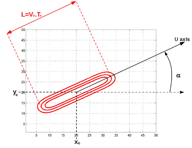
These functions and are what we call drifting PSF (DPSF). We call the one-dimensional moving Gaussian (or 1D MoG) function, while we name the two-dimensional moving Gaussian (or 2D MoG function). The geometry of the 2D MoG function and its main parameters are summarized in Fig. 1.
We note that the normalized 2D MoG function () is the product of a normalized 1D Gaussian () and a normalized 1D MoG function ().
In this paper, and allow us to represent the PSF of a moving source (such as asteroids, meteors, and artificial satellites) on a linear and a two-dimensional detector, respectively. As extensively shown in Veres et al., (2012), the function is one of the most accurate PSF models for extracting astrometric data from moving sources observed with a CCD sensor. We note that for photometry a more accurate PSF model has been proposed for moving source in Fraser et al., (2016).
3 CRLB behavior for moving sources observed with one-dimensional array detectors.
3.1 CRLB expression for the 1D MoG spread function
In statistics, the CRLB gives the lower bound for the variance of an estimated parameter: it can be represented as the inverse of the Fisher information, which characterizes the amount of information about this parameter contained in an observable random variable. MSL13 established the expression of the CRLB for the astrometric precision for a linear array detector, with the measurement noise driven by a Poisson distribution (the adoption of this probabilistic model is common in contemporary astrometry (e.g., in Gaia, see Lindegren, (2008))). The most generic expression for the CRLB given in MSL13 (their Eq. (11)) can be written as follows:
| (14) |
is the CRLB for the variance of the PSF center of a source observed with a one-dimensional array. The subscript allows identifying quantities relative to the pixel of index : represents the flux in pixel (in photo- on the detector), whereas the background flux in the same pixel is denoted by and includes contributions from the detector such as dark-current and read-out noise (), as well as contributions from the sky background (see Eqs. (22) and (37)). Throughout this paper, we assume for simplicity that is uniform (constant) under the source (and equal to in one pixel).
The function involved in Eq. (14) can be expressed by the integral over pixel of the one-dimensional PSF () of the source centered at as follows:
| (15) |
Where the integrals bounds and equal and respectively (with the coordinate of the center of pixel and the pixel width). The other parameters have the same definition as in Sect. 2: is the source total flux and the normalized PSF. We note that our function that we defined in the previous section is the same as the function adopted by MSL13 for the normalized PSF to express in Eq. (14).
3.2 Qualitative behavior of the CRLB expression for a linear detector.
In this subsection, we study the behavior of Eq. (16) when the background in each pixel follows Eq. (22), which corresponds to a realistic expression for the background on a CCD during an astronomical observation,
| (22) |
where is the sky-brightness component of the background (in units of /arcsec), while and are the dark current (mostly negligible for modern optical semi-conductor detectors) and the standard deviation of the read-out noise of the detector (in ), respectively. We note that the requirement of a realistic estimator for the noise variance and a noise following a Poisson distribution to apply the CRLB expression (16) leads us to assume that the component of the background also follows a Poisson distribution.
The three solid lines (thin, normal, and bold) in Fig. 2 show the square root of the CRLB as a function of detector pixel size for a non-moving source with a Gaussian PSF centered on a given pixel and for an FWHM of , and ”, respectively. The dashed lines correspond to the same curves, but for a slow-moving source (with drifting parameter equal to the FWHM) whose PSF is also centered on a given pixel.
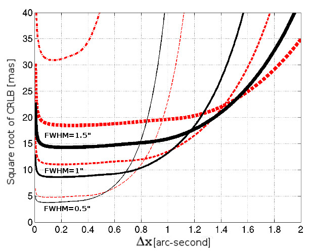
Figure 2 shows that for a given image quality, the CRLB minimum is understandably degraded by the motion of the source. We also point out that the shapes of the dashed curves (for a slow-moving source) and the solid curves (for a non-moving source) are similar. In particular, we can distinguish three regimes for the behavior of the CRLB according to the pixel size for a slow-moving source with a constant flux and a constant drifting parameter , as described below.
-
The oversampled phase: for pixel sizes considerably smaller than the image quality FWHM (in this case, arcsec), the background flux becomes preponderant. In this part of the curve, while the pixel size decreases, the part of flux that is due to the background increases compared to the flux of the source (since a part of the background flux is independent of the pixel size), and this leads to an increase in the CRLB (lower precision).
-
The undersampled phase: for pixel sizes larger than the image quality FWHM, the main part of the flux from the source is contained in very few pixels and the CRLB increases quickly. In the same way as for a non-moving source, the value of pixel size for which this degradation occurs largely depends on the centering of the spread function inside the pixel (see below).
-
The well-sampled phase between the two areas described above ( FWHM), where the CRLB reaches a quasi-constant floor. We note that when the contribution that is due to the source of the total flux decreases, the size of the well-sampled area also decreases (e.g., compare the shape of the lower dashed line with the upper crossed line, which is computed for a source ten times fainter, all else being equal). The reason is that as the background increases, the oversampled area extends to larger pixel sizes, while the undersampled area begins at an unmodified pixel size, close to the FWHM. Then, for a total flux that is largely dominated by the background, the “well-sampled floor” will collapse into a unique point corresponding to an optimal pixel size in which the CRLB reaches its minimum.
We now consider the behavior of the CRLB when the PSF is not centered on a given pixel. Figure 3 shows a set of curves corresponding to the CRLB versus pixel size for an FWHM of ”, for three different values of the source drift, and for different values of the PSF center inside one pixel. The lowest curves of this figure correspond - like the intermediate dashed lines in Fig. 2 - to the CRLB of a slow-moving source with = FWHM. As in the case of the stationary source (see MSL13), we see that the decentering effect on the CRLB of a slow-moving source is almost negligible in the oversampled and well-sampled domains, but it plays a leading role in the undersampled case when the pixel size exceeds the FWHM.
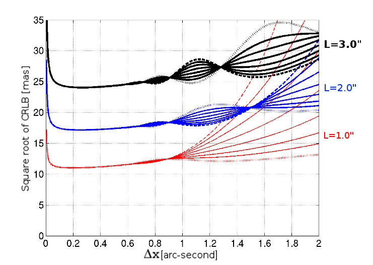
We now focus on the behavior of the CRLB for faster sources (i.e., for sources with a drifting parameter larger than the FWHM). As intuitively expected, we see in Fig. 3 that the larger the drift of the source, the larger the degradation of the CRLB. We also observe a number of significant oscillations of the CRLB values according to pixel size that are not present for stationary or slow-moving sources. The number and amplitudes of these oscillations increase with increasing speed of the source. Their amplitudes form an insignificant part of the CRLB value itself in the case of small pixel sizes (for oversampled and well-sampled sources this effect is negligible), but the contribution becomes important in the undersampled “intermediate” domain that is bounded by pixel sizes between the image quality FWHM and the elongation of the source drift. In the undersampled domain that is defined by pixel sizes larger than the drifting parameter, the effect that is due to oscillations disappears and the decentering effect dominates the behavior of the CRLB (as for stationary or slow-moving sources).
The oscillations of the CRLB that are observed for fast-moving sources are due to the numerical discretization of the source PSF (by the detector array) for which some resonances occur when the ratio between the pixel size and the drifting parameter reaches some specific values. Notably, we observe some peculiar localizations (pixel size values) for which the decentering effect is almost suppressed when the source is affected by a specific fast drift, while this effect is preponderant when the same source is stationary or affected by a slow drift (e.g., compare the behavior of the CRLB for sources with drift parameters of ” and ” at a pixel size of ” in Fig. 3).
These peculiar locations can be of particular significance when performing accurate astrometry of fast objects (e.g., near-Earth objects (NEOs), artificial satellites, space debris, or meteors) even with small telescopes whose pixel size can be substantially larger than the typical seeing. When the speed of the source is known, it is indeed possible (and advantageous) to adapt the exposure time to increase or decrease the drifting parameter such that the decentering effect is suppressed or minimized given the pixel size of the camera in use.
For undersampled sources, it is not possible to simplify the expression given by Eq. (16) of the CRLB (the same is true for stationary sources), since no continuous approximation is practicable to avoid the large effect of the detector-array discretization. Fortunately, the minimum value of the CRLB is not in the undersampled domain, and the effect due to oscillations and decentering can be neglected in the other two phases of the curves, and especially in the oversampled domain, which is further analyzed in the next subsection.
3.3 CRLB approximation in the oversampled case
In the oversampled case, as explained in MSL13, the CRLB can be simplified: the pixel width is considerably smaller than the FWHM of the PSF, and then Eq. (15) is well approximated by ; in addition, the sum over all pixels involved in Eq. (14) can be approximated by a continuous integral over the interval . We can then distinguish two limiting situations: the case when the background flux per pixel is clearly higher than the total flux of the source , in which case Eq. (14) becomes
| (23) |
And the case when the background flux per pixel is clearly lower than the total flux of the source , in which case Eq. (14) becomes
| (24) |
We note that even though these approximations have been developed by assuming a very small pixel size, the estimates and results deduced from them hereafter remain true in the well-sampled case with less accuracy, of course. This is especially visible in the next figures of this section, where the pixel size is consciously chosen to be relatively large (close to one-third of the FWHM).
To approximate the integrals involved in Eqs. (23) and (24) for a moving source, we first replace the normalized PSF by the 1D MoG function , and then we consider two distinct cases corresponding to slow- and fast-moving sources.
3.3.1 Sources with small drifting parameter
We first study the case when the elongation of the source (as a result of its drift) is small compared to the image quality FWHM. To achieve this, we replace the reciprocals of the integrals involved in Eqs. (23) and (24) by their Taylor expansions in the vicinity of a drifting parameter equal to zero (for details see Appendix A.2). Then, for a slow-moving source, Eqs. (23) and (24) of the CRLB in the oversampled regime become expression (3.3.1) when the background dominates the total flux, and expression (26) when the source dominates the total flux,
| (26) |
where is the normalized drifting parameter equal to .
The scale coefficients and of Eqs. (3.3.1) and (26) correspond to the two expressions given by MSL13 for a non-moving source for a weak (or faint) source (MSL13 expression (39)) and for a strong (or bright) source (MSL13 expression (42)), respectively.
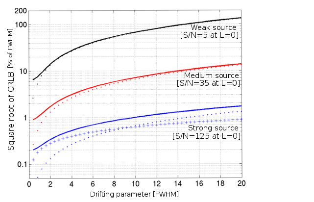
For a total flux dominated by the background, we observe for the weak source and the medium source in Fig. 4 that the estimator given by Eq. (3.3.1) (dotted lines) provides a correct approximation of the general behavior of the CRLB for a moving source with a drifting parameter smaller than or equal to about twice the image quality FWHM. Of course, the larger the background compared to the source flux, the smaller the difference between this estimator and the CRLB that is computed with the exact expression (16). For a source with a drifting parameter larger than two, this difference increases quickly and a better estimator is given by expression (27) below. For a drifting parameter equal to FWHM, the omission of -term in expression (3.3.1) already represents of the total value.
When the total flux is dominated by the source, that is, in the strong source case shown in Fig. 4, the estimator given by Eq. (26) (curve with the plus sign) provides an overall better approximation of the behavior of the CRLB than the estimator given by Eq. (3.3.1) (bottom dotted lines), as expected. This estimate remains correct until a source with a drifting parameter equal to about twice the image quality FWHM (for a drifting parameter equal to FWHM, the neglected higher order terms and in expression (3.3.1) already represent of the total value).
3.3.2 Sources with large drifting parameters
Second, we study the oversampled case when the drifting parameter of the source is large compared to the image quality FWHM. Accurate approximations of the integrals involved in Eqs. (23) and (24) exist in this case as well (see Appendix A.3). Then, for fast-moving sources, the two expressions of the CRLB in the oversampled regime become
| (27) |
| (28) |
Expressions (27) and (28) give good approximations of the CRLB in the oversampled and well-sampled areas even for a source with a relatively small drifting parameter (see Fig. 5).
The approximation is less accurate for a source with an intrinsic flux close to the background value. This is for instance the case of the medium source in Fig. 5. For a drifting parameter of FWHM, the difference in this source between the approximation given by expression (27) and given by the exact expression (16) is , but this difference decreases to less than for a drifting parameter of FWHM.
For the total flux dominated by the background flux, we observe that expression (27) corresponds to twice the term in of the Taylor expansion of the CRLB for a moving source with a small drifting parameter (see Eq. (3.3.1)). We also note that this expression is equal to the estimator given by MSL13 for a non-moving source in their Eq. (39), multiplied by the square of . In this case, evolves as .
For the total flux dominated by the source, expression (28) is equal to the estimator given by MSL13 for a non-moving source in their Eq. (42), multiplied by . In this case, evolves as the square root of .
Finally we note that for a moving source with a drifting parameter larger than twice the image quality FWHM observed in the oversampled or well-sampled regime, a generic estimator of the CRLB is given by the maximum of the two expressions (27) and (28). The use of this generic estimator is particularly recommended to estimate the CRLB of sources that can be considered as bright when stationary, but that become fainter with an increase in the drifting parameter (see, for instance, the strong source in Fig. 5).
3.4 Optimum exposure time for astrometry of a moving source.
For a stationary source, the relation between exposure time and astrometric precision (according to the CRLB estimators given by the constant terms in Eqs. (3.3.1) and (26)) is trivial. For a non-moving source, the longer the exposure time, the higher the integrated flux of the source, which leads to an improved astrometric precision (the only limit is the saturation threshold of the detector). However, for a moving source, this is no longer true. Here, the longer the exposure time, the higher the integrated flux of the source, but - and this is the main difference to the stationary case - the larger the detector-array area covered by the source (because the distribution of the source flux drifts). As a result, as we increase the exposure time of a moving source, we add a comparatively larger noise that is due to the areal increase in the background.
In this subsection, we use the previously developed CRLB expressions for a moving source to determine the optimum exposure time that allows reaching the best astrometric precision. We note that instead of the CRLB exact expression (16) itself, we often use its approximations in the oversampled regime here because the CRLB minimum value is reached for pixel size values for which these simplified expressions still give a valid approximation of the CRLB (see Sect. 3.3). As a cautionary note, the estimate of this optimum exposure time is not correct when the pixel size falls into the intermediate or undersampled regimes.
In this scenario, the background is time dependent, and its expression becomes
| (29) |
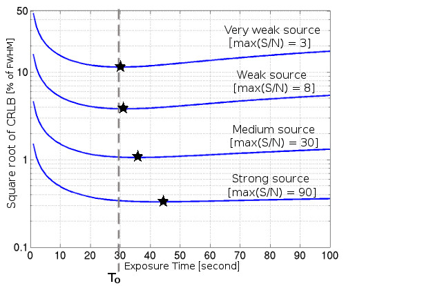
where is the background part depending on exposure time , while is the time-independent part. depends on , which is the sky component (in units of /arcsec/sec) and which is the dark-current component (in units of /sec). depends on which is assumed to be independent of exposure time. We recall that the relation between the source total flux and exposure time is , while the relation between source speed and its drifting parameter is given by . With these new notations, we compute the CRLB as a function of exposure time for four sources with a peak S/N bewteen and and a similar speed of ”/min. The pixel size, image FWHM, and background flux (whose RON component is negligible) are kept constant (see Fig. 6).
First we observe that the behavior of all CRLB curves is similar: with the increase in exposure time, the CRLB first decreases, then reaches a quasi-constant floor, and finally, unlike in the case of stationary sources, it reaches a turning point (where its minimum value is attained) and then starts to increase. When the RON is negligible (as for Fig. 6), the turning point is at an exposure time close to seconds, which corresponds to an elongation of the source drift close to the FWHM (equal to ” in the figure). When the RON component of the background increases, the turning point is located at a slightly longer exposure time.
We also note that the brighter the source, the longer the exposure time that is required to reach the minimum value of the CRLB (see the strong source case in Fig. 6). For the theoretical limiting case when the background flux is zero, this exposure time is infinity. An estimate of the corresponding minimum value of the CRLB in this theoretical case can be given accurately by expression (30), which is the limit when the exposure time approaches infinity in Eq. (28), which is valid for a high value of the drifting parameter,
| (30) |
Expression (30) is of particular significance. It gives a simple way to estimate an absolute limit for the astrometric precision of all moving sources with the knowledge of only three parameters, which are the FWHM, the flux of the source in electrons per second, and the source speed in arcseconds per second.
By contrast, the fainter the source, the smaller the size of the CRLB floor, and the more the optimum exposure time converges toward a lower limit that is close to the exposure time that corresponds to a drifting parameter that is equal to the image quality FWHM. We call the lower limit of the optimum exposure time (see Fig. 6) and the corresponding drifting parameter . We can calculate as a power series by considering the roots of the derivative of expression (23) with respect to the exposure time when is replaced by . Expression (23) in the oversampled area yields the limit of the expression (16) of the CRLB when the background dominates the total flux, and Fig. 6 shows that it is precisely in this regime that a lower limit of the optimum exposure time is achieved. Then, we can express as follows (see Appendix B for more details):
| (31) |
where is the exposure time corresponding to a drifting parameter that is equal to the image quality FWHM (), and measures the ratio between the time-independent and the time-dependent parts of the background flux for an exposure time equal to (). The numerical coefficients in Eq. (31) have been confirmed by an estimate of based on a binary search algorithm applied on the exact expression (16): for below , the agreement is better than one percent, but for larger than this expression of is no longer valid. In particular, this means that when the RON component is an important part of the background, the lower limit of the optimum exposure time cannot be given by Eq. (31) and has to be determined numerically from the Eq. (16).
To obtain an estimate of the CRLB value for an exposure time equal to , we replace the parameter by in expressions (3.3.1) and (26) for the case when the total flux is dominated by the background, and the case when the total flux is dominated by the source, respectively (these CRLB estimators can be used here since we have shown that they give correct results even for a drifting parameter equal to one and a half times the FWHM). We obtain the following two expressions:
| (32) | |||||
| (33) | |||||
When is used as exposure time and when the RON is a negligible part of the total background, we can deduce from Eqs. (32) and (33) that the degradation of for a moving source is between and of the of the same source with no motion observed during the same exposure time. When the RON is not a negligible part of the total background ( different from zero), the CRLB degradation that is due to the motion of the source is slightly larger (since is longer).
When the total flux is dominated by the source (as for the strong sources shown in Fig. 6), the CRLB of a moving source can reach a value slightly below the value given by expression (33). From the comparison between this expression and Eq. (30), however, we deduce that the maximum possible improvement for is , and only for a theoretical measurement without background, and with an exposure time equal to infinity.
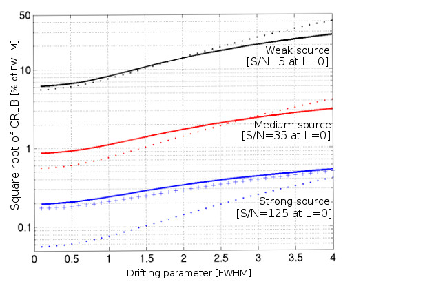
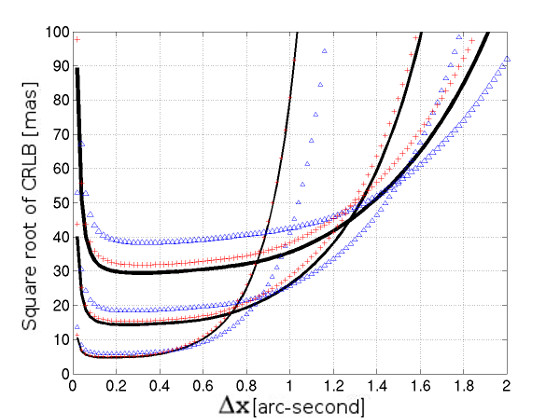
In order to check the validity range of the previous expressions, we compute with the help of a binary search algorithm applied to Eq. (16) the exact minimum CRLB for moving sources with a speed of ”/min and with fluxes varying between /min and /min. These sources are observed with a CCD pixel size of ”, an image quality FWHM of ”, and with a sky-background component /arcsec/min (the dark and the RON background components are equal to zero). Depending on the source brightness, the peak S/N varies between and . Then, we plot in Fig. 7 for each S/N value the exact minimum CRLB value obtained by this numerical method (bold line) and their estimates with expression (32) (dots), with expression (33) (thin dashed line), and with expression (30) (thin solid line).
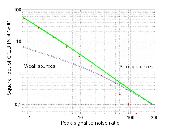
For weak sources (left part of Fig. 7) the exact determination and the estimate made with expression (32)
agree well. When the source is stronger (right part of the figure), the agreement is better with the estimate deduced from expression (33), and except for the strongest source of this example (), the value provided by this expression is below the exact minimum CRLB value. For the strongest source the estimator given by Eq. (33) is just above the exact value (less than higher). The unreachable limit given by expression (30) is always below the exact value and all the other estimates, as expected.
Optimum exposure time for a set of observations
Most of the time, the observation of a moving source consists of consecutive images of the source taken with a similar exposure time . If during (the duration of the whole data set) the meteorology, the instrumental conditions, and the linear motion of the target remain unchanged, then the lower bound of the final variance of the astrometric precision of the whole data set is given by (where is the variance of the astrometric precision of one independent image). Note that it is beyond the scope of this paper to develop a method to combine the single measurements. Hereafter we only assume that an ideal method exists and deduce a lower bound for the astrometric precision of the ”mean measurement”.
The CRLB formalism can help us to estimate the optimum exposure time of a single image, which maximizes the astrometric precision of a whole data set. Let be this optimum exposure time, the number of frames contained in the data set are , where is the time delay between consecutive exposures. Then, the CRLB for the whole data set equals (where is now the CRLB of one image).
In what follows we develop a method to graphically locate the optimum exposure time for a given source, when its characteristics ( and ) as well as the observational conditions (FWHM, , , , , and RON) are assumed to be known. We note that finding the optimum exposure time that minimizes is equivalent to finding the value of that maximizes the ratio of to , where , defined previously, is the exposure time corresponding to a drifting elongation equal to the FWHM. With the above notation, we can write this ratio as follows:
| . | (34) |
We note that the choice of the exposure time for the numerator of this ratio is arbitrary and that the same method can be applied with any fixed exposure time. The advantage of considering this ratio instead of itself is that this ratio is independent of the total duration of the data set. In return, with this method, is not an integer a priori, and will need to be slightly increased or decreased to reach the closest integer that minimizes .
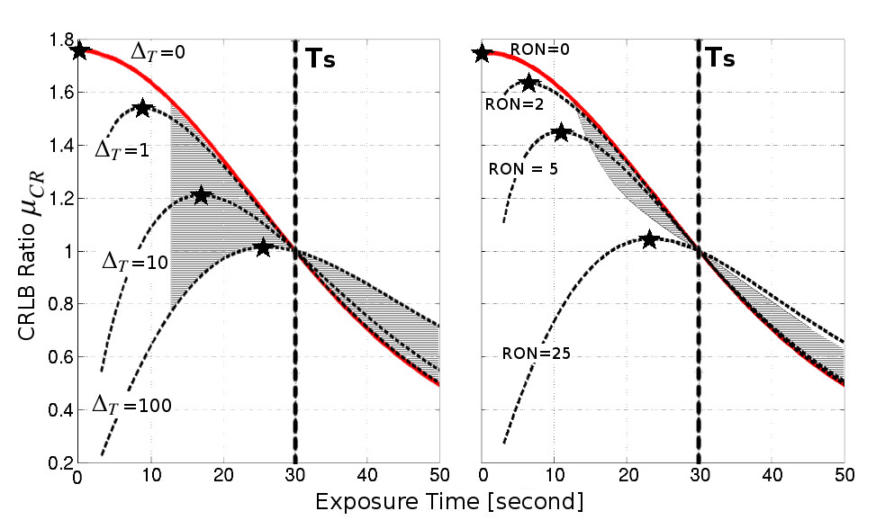
We compute and plot in Fig. 8 the CRLB ratio of Eq. (34) (where is replaced by its exact expression (16)) according to the exposure time for a moving source with a drifting speed of ”/min observed with an FWHM of ”. The vertical lines at seconds correspond to (which is close to , but independent of RON, in contrast to ). In the left panel of the figure, we assume that RON is zero while the time delay varies, and conversely, in the right panel of the figure, we assume that is zero while RON varies. The star symbols correspond to the maximum of the CRLB ratio, and the abscissa gives the values of corresponding to each condition.
We observe that the maximum of the limiting curve when RON and tend to zero (the two identical bold curves in the left and right panels) is reached for an exposure time equal to zero, which makes no sense. Another criterion has indeed to be taken into account: the optimum exposure time (according to the CRLB estimator) has to be long enough to allow the detection of the source. As a trivial example, we consider that a source is detected if the peak S/N is higher than a fixed threshold characterizing the reduction pipeline capacity (fixed to hereafter).
For instance, with the parameters of Fig. 8, the minimum exposure time needed to reach an S/N higher than is seconds when the RON is negligible (left panel), and it increases when the RON increases (for a RON larger than , the S/N is always below the threshold). Then, by adding this information concerning the detectability of the source in Fig. 8 (hatched areas), we can easily determine for each observational constraint a “realistic” exposure time for the whole data set by restricting the search of the CRLB ratio maximum to these hatched areas.
We see that increases quickly with the rise of (left panel) or with the rise of RON (right panel): with equal to only one-thirtieth of , already equals one-third of . We also observe that this increase seems bounded by . Indeed, is logically shorter than the optimum exposure time of a single image (minimizing ), and we have shown that even though this exposure time can be longer than (or ), the value of is already close to the minimum of . We note that this bound does not exist for a stationary sources.
We do not show a power series for (as done for in Eq. (31)) because the location of the maximum of Eq. (34) is the result of a complex interaction between several parameters. However, the simplest and more straightforward numerical approach - an estimate of that is based on a binary search algorithm applied to the search of the maximum of the CRLB ratio - allows us to compute and then to deduce the number of images that will optimize the CRLB of a whole set of observation of duration . This is particularly important when planning astrometric observations of moving targets. We note that This method can also be used without any modification to compute when the images are stacked before the reduction process (but the minimum exposure time for allowing detections is shorter since the S/N is multiplied by ).
4 CRLB behavior for sources observed with a two-dimensional sensor
This part extends the results of the previous section to two-dimensional detectors in three steps: extension of the generic CRLB expressions for these detectors, application of these expressions to a stationary source, and finally, in order to reach the main objective of our study, application of these expressions to the case of a source with linear and constant motion.
4.1 Generic CRLB expressions for astrometric precision with two-dimensional detector arrays
A two-dimensional array detector of columns and rows can be considered as a linear-array detector of pixels. Then, by keeping the same formalism as in the previous section, we can deduce from Eq. (14) the expression below which this corresponds to the CRLB for the astrometric precision along the -axis in the case of a two-dimensional detector array:
| (35) |
is the CRLB for the variance of the coordinate of the PSF center for a source observed with a two-dimensional array. The subscripts and now allow us to identify quantities relative to the pixel in column and row . The function represents the flux contained in the pixel that is located in column and row , and can be calculated through the integral of the normalized two-dimensional PSF () of the source centered at coordinates . The expression for is
| (36) |
where , , and (with and the pixel width along and respectively). The background flux in the same pixel is called . As previously, the background is uniform under the source (equal to in one pixel) and can be divided into three components: the and the dark current (), which are independent of the pixel size, and the sky-brightness component which was proportional to the pixel size in the one-dimensional case (Eq. (22)) and which is proportional to the pixel area now in the two-dimensional case (Eq (37)),
| (37) |
CRLB approximations for the oversampled case
Similar to the case of the one-dimensional detector-array, when the pixel sizes in X and Y are small compared to the image quality FWHM, the flux in one pixel given by expression (36) is well approximated by and the sums over all pixels present in CRLB expression (35) can be replaced by continuous integrals over the whole space. We can then distinguish two extreme scenarios: the case when the background flux per pixel is clearly higher than the total flux of the source (faint sources), in which case Eq. (35) becomes
| (38) |
And the case when the background flux per pixel is clearly lower than the total flux of the source (bright sources), when Eq. (35) becomes
| (39) |
More generally, hereafter, we denote as the CRLB for the astrometric precision along any direction in the reference plane of the CCD. The expression for would be given by Eqs. (35), (38), or (39) (depending on the case involved), with the derivative of (or ) with respect to replaced by the derivative with respect to (where is the component of the instantaneous PSF center along the -axis). For expressions (38) and (39), the integral over the whole space can also be performed with any coordinate system instead of the system adopted here since the pixel sizes are smaller than the FWHM.
4.2 Stationary sources on a two-dimensional array
The expression of the normalized PSF of a stationary source that is observed with a two-dimensional detector array is given by Eq. (2) of Sect. 2. Then, by using this normalized PSF in Eq. (36) to compute and its derivative and by substituting them into Eq. (35), we obtain the following expression for the CRLB along the -axis for a stationary source that is observed with a two-dimensional detector array:
| (40) |
where
| (45) |
Hereafter, we assume that the pixel sizes along and axes are equal ().
The three solid lines in Fig. 10 (thin, normal, and bold) computed with Eq. (40) show the square root of the CRLB as a function of detector pixel size for a non-moving source centered on a given pixel and observed with a two-dimensional detector for an FWHM of ”, ”, and ”, respectively. We note that the overall behavior of these three lines is very similar to the three solid curves plotted in Fig. 2 for a non-moving source that is observed with a one-dimensional detector and based on Eq. (21) of MSL13. In particular, the three distinct regimes (oversampled, well-sampled, and undersampled) also exist in the two-dimensional case. We can observe, however, that in the two-dimensional case the oversampled regime is slightly more extended, while the well-sampled area begins for pixel sizes that are slightly larger.
Oversampled case approximations:
The CRLB expressions (38) and (39) with as normalized PSF allow us to produce simplified expressions for the CRLB of a stationary source that is observed with a two-dimensional array detector (the values of the reciprocals of the integrals involved in Eqs (38) and (39) for are given in Appendix A.1 by the functions and , respectively). Thus, the expression (40) is well approximated by expression (46) when the background dominates the total flux, and by expression (47) when the source dominates the total flux,
| (46) |
| (47) |
where and correspond to the CRLB expressions given by MSL13 in their Eqs. (39) and (42), respectively, for a stationary source that is observed with a one-dimensional detector. When the background dominates the total flux, we observe that the CRLB in the two-dimensional case is equal to the CRLB in the one-dimensional case multiplied by a factor that is inversely proportional to the pixel size and larger than 1 when FWHM. This factor explains that the degradation of CRLB in an oversampled regime occurs for a larger pixel size in the two-dimensional case than in the one-dimensional case. When the source dominates the total flux, the CRLB expression remains unchanged.
4.3 CRLB of a moving source observed with a two-dimensional digital-detector array
Finally, we present in this subsection the CRLB behavior for a moving source observed with a two-dimensional detector array. As a PSF of the moving source, we use , the 2D MoG function given by Eq. (3) and presented in Sect. 2. This function is not circularly symmetric, and therefore the CRLB is not the same along all directions. However, compared to the stationary case, the main modification of the CRLB behavior is, of course, in the drifting direction. Thus we first study the CRLB along the drifting direction and show the similarities and differences with the results obtained in Sect. 3 for a linear detector. Then, we study the CRLB along the direction normal to the motion of the object - which is of course not present in the linear case.
4.3.1 CRLB along the drifting direction
Following the conclusions of Sect. 4.1, the generic expression for the CRLB along the drifting direction (i.e., along the -axis) is given by expression (35), where the normalized PSF is replaced by and where the partial derivative of with respect to is replaced by the derivative of with respect to . The resulting expression for the CRLB along the drifting direction is the following:
| (48) |
where now
| (52) |
In contrast to the previous CRLB expressions, the explicit integrals cannot be easily avoided here because the integrals have to be performed in the pixels frame (i.e., -coordinate system), while the 2D MoG function is only multiplicatively separable in the -coordinate system. It follows from this that the computing time for this CRLB expression is longer than for the previous one.
Equation (48) can be seen as an extension of the CRLB expression (16) for a two-dimensional array detector, and the next figure allows us to compare the behavior of these two CRLB expressions.
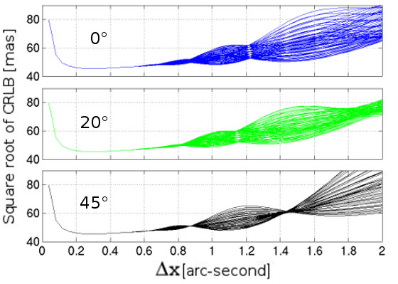
Figure 9 shows three sets of curves corresponding to the CRLB computed with Eq. (48) versus pixel size for an FWHM of ” and drifting parameter of ” for different values of the PSF offset from the pixel center and for three different values of the inclination angle (, see Fig. 1) of the DPSF.
We first compare the curves for in the top row of Fig. 9 (DPSF drift aligned with the detector -axis) with the top curves (”) of Fig. 3. For these two graphs, the CRLB is computed for the same source as was observed in the same conditions, but with a two-dimensional detector array in the first case (Eq. (48)) and with a one-dimensional one in the second case (Eq (16)). We see that the overall behavior of the CRLB along the drifting direction for a moving source is fairly similar in the two cases. It follows that most of the results and conclusions of Sect. 3 can be extended for observations performed with two-dimensional detectors.
In particular, the same distinct areas remain visible: the oversampled area where the CRLB decreases when pixel size increases, the well-sampled area where the CRLB remains constant (for pixel sizes close to the FWHM half-value), the intermediate area where the CRLB oscillates (for values of the pixel size between the FWHM and the drifting parameter ), and the undersampled area where the CRLB increases when the pixel size increases (for a pixel size ” not shown in Fig. (9)).
Concerning the impact of pixel decentering on the CRLB behavior, the two-dimensional case is similar to the linear case: in the oversampled and well-sampled areas, the pixel decentering effect is almost negligible, while in the intermediate and undersampled areas, the CRLB behavior is strongly affected by this effect. However, the specific pixel size values of the intermediate regime where the CRLB values were almost not affected by the decentering effect seen in the one-dimensional case (as for a pixel size value of ” for the top source in Fig. 3) are more affected by the decentering effect in the two-dimensional case. The reason is that with a two-dimensional detector, the pixel decentering of the PSF has not one, but two degrees of freedom, which are represented by two offsets along the X- and Y-axes, and there is no reason for these two decentering components to be counterbalanced by the drift of the source for the same pixel size. There is one exception, however: when the inclination of the DPSF with respect to the X axis of the CCD frame equals , the decentering along both axis vanishes for the same pixel size values (see, for instance, the bottom curve of Fig. 9 at the pixel size of ”). This configuration can be particularly advantageous when an observation of a moving target has to be planned in an undersampled regime.
Finally, we also note, as was the case for the linear detector case, that the minimum value reached by the CRLB is not in the undersampled area of the plot, and that the combined effect that
is due to decentering and orientation of DPSF can be neglected in the oversampled and well-sampled areas.
Oversampled case approximations:
We can produce accurate approximations of Eq. (48) for a two-dimensional detector that observes in an oversampled regime by using as the normalized PSF in Eq. (38) (when the background dominates the total flux), and in Eq. (39) (when the source dominates the total flux) and by replacing the derivatives with respect to by the derivatives with respect to . Moreover, following a remark of Sect.4.1, we can compute in the -space instead of the -space the two integrals of Eqs. (38) and (39) (whose reciprocals are denoted and , respectively).
The approximations of these reciprocals are given in Appendix A.2 (when the drifting parameter is small) and in Appendix A.3 (when the drifting parameter is large). When the drifting parameter is small (FWHM), expressions (38) and (39) for the CRLB along the drifting direction become
| (54) |
respectively, while when the drifting parameter is large (FWHM), the expressions become
| (55) | |||||
| (56) |
Here we recall that the normalized drifting parameter is equal to and that the background follows the two-dimensional expression (37) and not Eq. (22) that was used in the linear case.
We first observe that when the source dominates the total flux, expressions (54) and (56) are identical to expressions (26) and (28), respectively, that were used in Sect. 3.3 for the source that was observed in the same regime with a linear detector. When the background dominates the total flux, expressions (4.3.1) and (55) can be deduced from approximations (3.3.1) and (27) for a linear detector by multiplying them by .
Thus, all the remarks concerning the behavior and the precision of
the CRLB approximations given for a linear detector in
Sect. 3.3 can be trivially
extended for a two-dimensional detector. In particular, and in a
consistent way, for a slowly moving source, the limit of
the CRLB expressions (4.3.1) and (54) when
approaches zero are equal to expressions
(46) and (47), respectively, of a stationary source in the
same regime. Similarly, when increases, the four CRLB
approximations of this section are logically degraded compared to the
CRLB expressions for a stationary source in the same regime.
Optimum exposure time:
We recall that in Sect. 3.4 we defined the optimum exposure time as the exposure time that minimizes the CRLB for a moving source, and we distinguished the optimum exposure time for an isolated image from the optimum exposure time of one image contained in a set of N images with a fixed total duration .
Concerning the optimum exposure time for an isolated image, all the results obtained in that previous subsection were based on approximations of the CRLB in the oversampled regime. In this regime, the CRLB expressions for a moving source observed with a two-dimensional detector and with a linear one differ only by a scale factor that is independent of time, therefore all the results of Sect. 3.4 can be easily generalized to the two-dimensional case. Nevertheless, for a two-dimensional detector array, the background flux , instead of obeying Eq. (29), follows Eq. (57),
| (57) |
The unit of the sky component () is now /arcsec2/sec.
In particular, from a quantitative point of view, the expression for the ultimate lower limit for the astrometric precision of a moving source (30), as well as the expression of the lower limit for the optimum exposure time (31), remain unchanged in the two-dimensional case. Similarly, expression (33) of the CRLB when the source dominates the total flux for an exposure time equal to is still valid in the two-dimensional case, while expression (32) of the CRLB when the background dominates the total flux has to be multiplied by a factor for the two-dimensional detector array.
Similar as in the one-dimensional case, if the lower limit is used as exposure time and if the RON is negligible, the degradation of the CRLB for a moving source along the drifting direction is therefore larger by and than the CRLB for the same source when it is observed with no motion and during the same exposure time. When the RON is not a negligible part of the total background, the CRLB degradation caused by the motion of the source will be slightly larger. When the total flux is dominated by the source, the CRLB of a moving source can reach values slightly below the value given by expression (33), but the maximum possible improvement is and only for an (ideal) measurement without background and with an exposure time equal to infinity.
Concerning the optimum exposure time for a whole set of images with a fixed total duration , the method applied for a linear detector is directly applicable for a two-dimensional detector by using Eq. (48) to model (instead of Eq. (16)) in expression (34) of the CRLB ratio. A binary search algorithm applied to the localization of the maximum of this new CRLB ratio expression allows us to compute by optimizing the CRLB of the set of images observed now with a two-dimensional detector array.
4.3.2 CRLB along the direction normal to the motion
For moving sources observed with a two-dimensional detector, the behavior of the CRLB along the direction normal to the motion is not adequately represented by the expressions developed for stationary sources (and this even though the cross-section of the DPSF along this direction is similar to the PSF of stationary sources). In the two-dimensional case, the measurement of the CRLB along the direction normal to the motion indeed depends on the number of pixels covered by the PSF along the direction perpendicular to this measurement (i.e., the direction of the motion). An increase in the underlying number of pixels in the direction of motion decreases the S/N without adding any information for the PSF centering along the direction normal to the motion. Since the underlying number of pixels along the direction of motion is directly related to the source-drifting parameter , the expression of the CRLB along the direction normal to the motion should depend on as well. All other things remaining equal, the smaller , the higher the S/N and the smaller the CRLB along the direction normal to the motion. The lowest value of the CRLB in this case would be reached when the drifting parameter equals zero (i.e., for the stationary source).
The generic expression for the CRLB along the direction normal to the motion (i.e., along the -axis) can be deduced from expression (35) by replacing by and the derivative with respect to by the derivative with respect to . Then, the expression of the CRLB along the direction normal to the motion is the following:
| (58) |
where now
| (62) |
For similar reasons as those given in the case of the CRLB along the drifting direction, in expression (48), the explicit integrals cannot be easily avoided here.
As expected, we see from Eq. (58) that the CRLB expression along the direction normal
to the motion depends of the source-drifting parameter (through and as defined in Sect. 2).
Oversampled case approximations:
We can give accurate approximations for the CRLB along the direction normal to the motion by using the 2D MoG function and by now substituting the partial derivative with respect to by the one with respect to in Eqs. (38) and (39). The approximations of the reciprocals of the two integrals involved in Eqs. (38) and (39) are given in Appendix A.2 (for a small drifting parameter) and in Appendix A.3 (for a large drifting parameter). The reciprocals of the integrals involved in Eqs. (38) and (39) are denoted and , respectively.
First, when the source dominates the total flux, the function is independent of the drifting parameter and equals , which corresponds to the same integral computed with a normalized PSF corresponding to a stationary source observed with a two-dimensional detector (see Appendix A.2 and Sect. 4.2)). In the oversampled case, when the background component is insignificant in comparison to the source flux, we see that the CRLB of a moving source measured along the direction normal to the motion is identical to the CRLB of the corresponding stationary one and the CRLB expression is given by Eq. (63),
| (63) |
Second, when the background dominates the total flux, the function depends on the source-drifting parameter through a scale factor that involves the integral over the whole space of the square of the 1D MoG function (Appendix A.2). As previously, to compute this integral analytically, we have to distinguish two cases: slow-moving sources, and fast-moving sources (see Appendix A.2 and A.3 for details), and the corresponding CRLB expressions become
| (65) |
respectively. As expected, the limit of the CRLB expression (4.3.2) when approaches zero is equal to the CRLB expression (46) of a stationary source in the same regime. When increases, expressions (4.3.2) and (65) are degraded compared to the CRLB expression of a stationary source, but less so than the CRLB measured along the drifting direction as represented by expressions (4.3.1) and (55), respectively.
When we substitute in Eq. (4.3.2) by the normalized optimal drifting parameter , we obtain the minimum degradation of the CRLB along the direction normal to the motion for the case when the background dominates the total flux. We obtain
| , | (66) |
where is now computed with and of Eq. (57).
By using Eq. (66), we conclude that if the optimum exposure time is used as exposure time, the maximum degradation of the CRLB along the direction normal to the motion is larger than the CRLB of the corresponding stationary source when the RON is negligible and slightly larger if it is not. For a bright sources, this degradation tends to zero, as shown by Eq. (63).
To conclude this section and to summarize the main results obtained for the limit of the astrometric precision for moving sources observed with a two-dimensional detectors, we present in Fig. 10 the CRLB behavior for a circularly symmetric source in the stationary case and in the moving case. For moving sources, we consider that the exposure time is the optimum exposure time presented previously, which means that the drifting parameter equals the optimum drifting parameter .
All other things being equal, we represent in Fig. 10 (for three different values of image quality FWHM) the behavior of the CRLB in the stationary case (based on Eq. (40)) and the behavior of the CRLB along two directions in the moving case: along the drifting direction (based on Eq. (48)), and along the direction normal to the motion (based on Eq. (58)).
We see that with this optimum exposure time, the CRLB overall behavior is very similar in both the moving and the stationary case. In particular, the CRLB oscillations visible in the intermediary-sampled regime for moving sources are not present here (this is due to the choice of exposure time, which leads to a drifting parameter below the FWHM, while this intermediary regime only appears for drifting parameters larger than the FWHM).
For the same FWHM, the CRLB minimum values for stationary as well as for moving sources in Fig. 10 are reached in the well-sampled area. The CRLB minimum value for a stationary source is always lower than that of a moving source. However, the minimum value for the CRLB along the direction normal to the motion is noticeably closer to the stationary one than the CRLB along the drifting direction: for the three sources in Fig. 10, this degradation of the CRLB minimum value amounts to around along the direction normal to the motion and to around along the drifting direction. Even though the minima of the CRLB are reached for relatively large pixel sizes (close to one-third of the FWHM), these percentages are in full agreement with the interval of degradation deduced from the CRLB approximations in the oversampled case when the exposure time equals and when the RON is negligible (i.e., between and for the CRLB along the drifting direction, and between and for the CRLB along the direction normal to the motion). This also visually confirms that the estimators developed in the oversampled case for slow-moving sources still give a good approximation in the well-sampled case (the estimator for CRLB along the drifting direction is given by the maximum of the two expressions (4.3.1) and (54), while the estimator for the CRLB along the direction normal to the motion is given by the maximum of the two expressions (4.3.2) and (63)).
5 Comparison with astronomical observations.
In the previous sections, several theoretical predictions have been derived for the limit of the astrometric precision that can be reached for both stationary and moving sources that are observed with digital-detector arrays. For stationary sources, the cornerstone of our analysis is Eq. (40), which gives the expressions for the CRLB along any direction. For moving sources, our results are based upon the two Eqs. (48) and (58), which give the expression of the CRLB along the direction parallel and normal to the source drift, respectively. In this section, the theoretical results derived using these equations are compared to the results of astrometric reductions performed on simulated and real astronomical observations of stationary and moving sources detected with CCD-sensors.
The astrometric reduction process encompasses the detection of all sources in an image above a specified threshold, determining for each source their and photocenter positions, their total flux, and the value of the image quality FWHM by fitting a 2D MoG function with an unweighted least-squares algorithm (LSA hereafter). The drifting parameters and the angle of the MoG functions are assumed to be known. These tasks are performed by using the GBOT astrometric reduction pipeline (Bouquillon et al.,, 2015), which is one of the tools developed for the GBOT satellite tracking project of ESA’s Gaia spacecraft, see Sect. 5.2. For each determination of a stellar photocenter, the GBOT reduction pipeline also provides two estimates, and , that correspond to the astrometric precision along the drifting direction and along the direction normal to the motion, respectively. These estimates are the standard deviations provided by the LSA through the PSF fitting process. In the next subsection we use simulated astronomical images to first demonstrate the quality of these estimators, and second, to compare the CRLB expressions of previous sections with the astrometric precision achieved by the GBOT image analysis.
5.1 Comparison with simulated data.
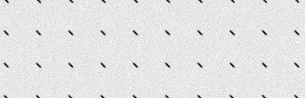
Three sets of simulated images with drifting sources in each image were created. An example of these images is given in Fig. 11. All the objects of a given image are similar (motion, FWHM, total flux, background, etc.). In a given set, the only difference between the objects of two distinct images are their drifting parameter (which varies, taking 21 different values between zero and ten times the FWHM). The total flux of each object in set is , in set it is , and in set it is . For all the images, the background mean value is , the pixel size is ”, and the FWHM is . At the end of this image creation process, we added noise following a Poisson distribution. The peak S/N of the objects of sets , and are , and respectively, in the stationary case and , and respectively, when FWHM.
The astrometric reduction of all these simulated images is performed with the GBOT pipeline, as explained in the introduction of this section. The results are summarized in Fig. 12 for fast- and slow-moving sources. This figure shows the astrometric errors, their GBOT estimates, and the corresponding CRLB values (in percent of the FWHM) with respect to the drifting parameter (in units of the FWHM): the top panel shows the astrometric error along the direction of motion (), while the bottom panel shows the astrometric error along the direction perpendicular to the motion (). The lower curves are for the sources of set , the medium curves for the sources of set , and the upper curves are for the sources of set .
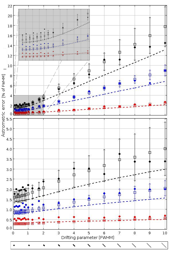
Each filled circle depicts the standard deviation of the differences between the known photo-centers and those estimated by the GBOT reduction pipeline for the similar objects of one simulated image. Each open square and each corresponding error bar show the mean value and three times the standard deviation, respectively, of the astrometric uncertainties estimated by GBOT for the objects of one image. These figures show that the estimates provided by the GBOT pipeline are quite robust: the majority of the true astrometric errors (filled circles) are within the error bars derived from the GBOT estimates. It seems that the quality of the estimates is slightly poorer for the brightest sources (bottom curves) or when the true astrometric error is very small (below of the FWHM).
For a drifting parameter close to four times the FWHM (similar to the case of the moving objects in the real image used in the next subsection), we see from Fig. 12 that the GBOT estimates are quite robust, and we observe that only for the brightest sources the estimate of the astrometric error along the direction normal to the motion overestimates the true astrometric error by about . This is most likely related to the loss of optimality (in the CRLB sense) of the LSA parameter estimating method, as recently demonstrated by Lobos et al., (2015) (see especially their Eq. (26) in proposition 3, and their Fig. 4).
For each simulated image we can also compute the corresponding CRLB values along the drifting direction (with the help of Eq. (48)) and in the direction normal to the motion (with the help Eq. (58)). The dashed lines correspond to these CRLB values, which are, from a theoretical point of view, the lower limits of the true astrometric errors, regardless of the centroiding method used. We note here that it can indeed be proven that the CRLB is theoretically unreachable in the context of digital detectors with Poisson noise, as demonstrated by Lobos et al., (2015) (see Sect. 3.1, “Nonachievability” and, in particular, their proposition 2).
As expected, we see that the theoretical CRLB values (dashed lines) are below the true astrometric errors (filled circles) computed from the centroiding performance of the GBOT reduction pipeline in all the cases. We also observe that the degradation of the GBOT true astrometric errors with respect to the drifting parameter is fully consistent with the CRLB overall expected behavior. Finally, we note that the differences between the two are small, but that improvements of the centroiding method accuracy are still possible (especially when the true astrometric error is small, below of the FWHM). We are currently working on implementing an algorithm within GBOT that is based on a maximum likelihood estimate, which we expect it will render better results when the S/N is high (Lobos et al., (2015), see especially their Fig. 8), this will be reported in a future paper.
In summary, our numerical results demonstrate the adequacy of the centroiding performance of the GBOT reduction pipeline (since the observed accuracies are close and in good agreement with the CRLB). Reciprocally, we validate the CRLB expressions (48) and (58) in the cases of moving sources observed with a two-dimensional array. They also demonstrate the robustness of the astrometric centroiding uncertainty estimate provided by GBOT. This was a necessary step before we proceed to the comparison of the CRLB expressions with true astronomical images of moving sources because in the real case, we do not have access to the true astrometric errors, but only to the GBOT estimates of astrometric uncertainties.
5.2 Comparison with real images.
For this aim, we selected astronomical observations performed with the VLT Survey Telescope (VST) of the European Southern Observatory (ESO), which is a 2.6 m wide-field optical survey telescope located on the VLT platform at Cerro Paranal, Chile. This telescope is equipped with one focal plane instrument, OmegaCam, a large-format (16k16k pixels) CCD mosaic camera with a large corrected field of view of . The observations were obtained in the framework of the GBOT campaigns (see Altmann et al., (2014) or Jordan and Altmann, (2013) for more details). The aim of these campaigns is to track the Gaia satellite to improve the accuracy of its orbit determination. Since the Gaia satellite is faint and moves relative to the reference frame defined by the background stars, the telescope tracking is locked on the Gaia speed. This tracking mode allows recording Gaia as a stationary source in the CCD frame (allowing a better precision of the photocenter determination, as extensively shown in this paper). On the other hand, this means that the - stationary - stars are moving sources in this frame, and their images on the CCD are elongated (see Fig. 13).
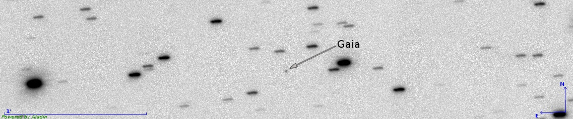
The image selected here has been taken at the very beginning of the mission, before Gaia settled in its operational orbit around Sun-Earth L2. The reason for this choice is that the apparent mean speed of Gaia after arrival at its final location near L2 as seen from Earth at night is usually around 0.02”/sec, while in this image the speed of Gaia is about 0.063”/sec. Thus, these data allow us to study the behavior of faster sources than the observations performed after Gaia settled in its final orbit.
In this image, the mean quality FWHM is ”. The exposure time was seconds, Gaia is stationary with respect to the CCD-frame, and the star’s motion with respect to the CCD frame is of the same amplitude and opposite to the motion of Gaia in relation to the star frame. This means that the stellar motions are oriented with an angle degrees with respect to the -axis of the CCD, and their drifting parameter is ” (which corresponds to a normalized drifting parameter of ). The mean standard deviation of the image background noise is ADU/pix. The detector has negligible dark-current and . Its gain is . The pixel size is ” (lower than one-third of the FWHM), which places this image between the oversampled and the well-sampled regime.
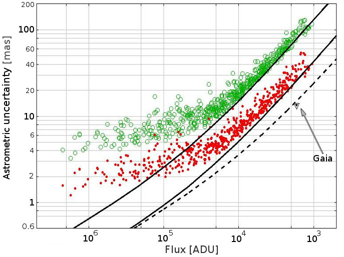
The great advantage of this image (with the stars being the “moving sources”) for this particular study is that it provides many sources with very different S/N, but with the same apparent motion (same apparent speed and direction) and the same instrumental and meteorological conditions (same image quality FWHM, same background noise, etc.).
In the same way as for the simulated images presented in the previous subsection, we performed the star centroiding determination by using the GBOT astrometric reduction pipeline with the MoG function as DPSF. As mentioned previously, the drifting parameters and angle of the MoG function are assumed to be known. Their values are those mentioned above and are deduced from the ephemeris of Gaia. To avoid including astronomically extended objects in our analysis, we only keep those objects detected by the GBOT reduction pipeline for which the fitted FWHM equaled the mean image seeing with a margin of error of . For Gaia, which is a stationary source in this image, we fit a circularly symmetric two-dimensional Gaussian.
The astrometric results of the reduction described in the previous paragraph are presented in Fig. 14. This figure shows the GBOT estimates of the astrometric uncertainties and for all the stars (and for Gaia) as a function of flux. The open and filled circles are for stellar and , respectively (the open and filled diamonds are for Gaia’s and ). As expected, we see that all else being equal, the brighter the source, the smaller the two uncertainty estimates for and of the star positions along the and axes. We then note that for every moving star, is always larger than , which means that the degradation of the astrometric precision is larger along the drifting direction than along the direction normal to the motion, as we discussed in the previous sections. For Gaia - the stationary source - the two uncertainty estimates and have the same value since a circular symmetric Gaussian has been fit. For stars with fluxes similar to that of Gaia, the uncertainty estimates of drifting sources (i.e., stars) are clearly larger than those of Gaia (whether it is along the drifting direction or perpendicular to it). Finally, we observe two distinct regimes for in comparison to : for bright sources the astrometric error is slowly degraded when the flux decreases, while for faint sources this degradation is faster. For this image, the bifurcation between these two regimes is for a source flux of around ADU (which corresponds to an S/N ).
We now compare the uncertainty estimates of this image with the CRLB expressions presented in the previous section. The bold and thin solid lines plotted in the same figure are computed by using expressions (48) and (58) of the CRLB along the and directions, respectively. The dashed line is based on Eq. (40) of this paper, representing the CRLB of a stationary source observed with a two-dimensional array detector. We see, as expected, that the bold solid lines represent the lower limit of the of the drifting sources (open circles), while the thin solid line is the lower limit of the of the drifting source (filled circles). We also see that in the regime of faint sources, the difference between CRLB expressions and the uncertainty estimates is very small. Similarly, for equivalent flux values, the difference between the uncertainty estimate of the stationary source (Gaia) and the uncertainty estimates along the direction normal to the motion of the drifting sources (stars) is clearly explained by the difference between expressions (40) and (58).
In the regime of bright sources, we observe from Fig. 14 that the differences between the CRLB expressions and the GBOT uncertainty estimates increase with the rise of the source brightness (visible in the left part of Fig. 14). This is likely due to two effects that should be studied in more detail, namely, (a) the choice of the LSA method, which is well-adapted for estimating source parameters for a low S/N (as is the case of the target, Gaia), but not for bright sources, as explained in detail in Lobos et al., (2015) (see also Sect. 5.1), and (b) because of a difference between our adopted DPSF fitting processing and the CRLB theory developed in this paper. We not only estimate one coordinate of the source photocenter (as assumed in the theoretical sections of this paper), but four parameters: the two coordinates of the photocenter, the total flux, and the FWHM.
Finally, we also note from Fig. 14 that for both faint and bright sources, the ratio of the two uncertainty estimates, and , seems to be approximately constant for the drifting sources, in very good agreement with the ratio of their respective CRLB given by Eqs. (48) and (58). This is visually confirmed in the upper part of Fig. 15, where the to ratios are plotted (with circles) as a function of source flux for all the stars detected in the VST image. The dashed curve is the corresponding CRLB ratio. In this figure, we clearly see that a large majority of the star uncertainty ratios are along the line of the corresponding CRLB ratio, with a better agreement in the regime of faint sources. We also note that for several faint source (less than ), there is an increase of the ratio values that we cannot currently explain.
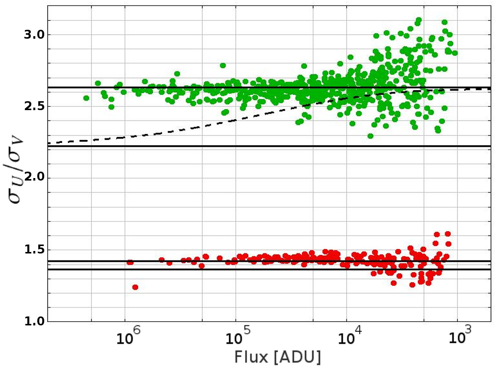
With the aim of validating the CRLB approximations given in this paper, we deduce the following simple expressions for the CRLB ratio by using the simplified expressions given in Sect. 4 for Eqs. (48) and (58). For fast-moving sources (as in the case of the VST images of January 6, 2014), the CRLB ratio can be approximated by the following two expressions:
| (67) |
| (68) |
Expression (67) (valid for fast-moving faint sources) is based on the ratio of Eqs. (55) and (65), while expression (68) (valid or fast-moving bright sources) is based on the ratio of Eqs. (56) and (63). The numerical values are for the GBOT-VST image of January 6, 2014, for which equals . We call this image .
On the other hand, for slow-moving sources, the CRLB ratio can be approximated by the following two expressions:
| (69) |
| (70) |
Expression (69) (valid for slow-moving faint sources) is based on the ratio of Eq. (4.3.1) and (4.3.2), while expression (70) (valid for slow-moving bright sources) is based on the ratio of Eqs. (54) and (63). As these expressions are for slow-moving sources, it is not possible to compare them with the error estimates of the VST image , where the star’s drift is significant. Instead, for this aim, we selected another GBOT-VST image, taken on May 2, 2015, with a smaller drifting parameter equal to (we call this second image ). Then, we performed the astrometric reduction in a similar manner as for the previous VST image, and we plot in Fig. 15 the to ratios (with filled circles) for all its drifting stars. We also plot the two horizontal lines that correspond to expressions (69) and (70) for (the numerical values given in the right part of these expressions are of course computed for the drifting parameter of this second image).
Figure 15 shows that as expected, all the curves and marks corresponding to the fast-drifting sources of the image are in the upper part of the diagram, largely above those that correspond to the slow-moving sources of the image . The smaller the drift, the smaller the difference between the two uncertainty estimates (or the CRLB values) along the and the axes, as extensively discussed in the previous sections. For the fast-moving sources of (upper part of the figure), we see (as expected) that the exact expression of the CRLB ratio (dashed curve) converges toward expression (68) for bright sources and toward expression (67) for faint sources (the two upper horizontal lines). We did not plot the exact expression of the CRLB ratio for the slow-moving sources of to avoid crowding in the figure, but in this case, it converges toward expression (70) for bright sources and toward expression (69) for faint sources (the two lower horizontal lines), as should be the case. This confirms that these approximate expressions for the CRLB in the case of a two-dimensional array detectors are indeed correct.
Concerning the ratio of the uncertainty estimates along the and axes, Fig. 15 shows that for both fast- and slow-moving sources, they are in the areas defined by their respective CRLB approximations (horizontal lines), but with a greater accumulation of points along the upper horizontal lines that correspond to the CRLB ratio approximation for faint sources. In fact, of the ratios of the error estimates for all stars are in an interval of around the CRLB ratio values computed under the faint source approximation.
We note that these last Eqs. (67), (68), (69), and (70) are particularly interesting since they allow us to estimate the relative difference of the centroiding precision quite accurately along the drifting direction and along the direction normal to the motion, without knowing anything except the source drifting parameter .
All these comparisons with both real and simulated data prove the usefulness of the CRLB expressions presented in this paper in characterizing the astrometric performance of moving sources that are observed with digital sensors.
6 Conclusions.
Following the earlier study of MSL13, we have extended their results to include not only the more realistic case of a two-dimensional detector array, but also explored the CRLB for moving objects. We have examined various different plausible observational scenarios: over-, well-, and undersampled pixel scales, and bright and faint objects (with respect to the background level). In several interesting regimes we were able to simplify the mathematics and obtain closed-form analytical equations for the CRLB, which led to expressions that can be used to analyze data in a very straightforward way. Thus we end up with a set of equations that allows us to determine the ultimate limit of the astrometric quality for astronomical data obtained with digital sensor arrays, today the most common type of detectors in optical astronomy. These expressions were validated by extensive comparisons with astrometric reductions that were performed on several sets of both simulated and real astronomical images. We note that the ultimate limit of the astrometric precision can be also deteriorated by several effects that we did not examine in the current paper, such as the quality of the reference catalog that is used for the calibration or shutter-timing errors.
One of the interesting and new results of our analysis is that the maximum positional precision as predicted by the CRLB exhibits important oscillations when the pixel size falls between the image quality FWHM and the elongation of the source drift, probably because of the discretization of the source PSF by the detector array. For very small pixels or for severely undersampled images, these oscillations disappear. We provide a simple recipe to avoid these oscillations if the speed of the source is known (see Sect. 3.2).
Another unexpected and very useful result of this study is that it provides a simple method for computing an optimum exposure time that minimizes the astrometric uncertainty of a drifting source that is observed with one- and two-dimensional array detectors (see Sect. 3.4). This method should be particularly useful for planning astrometric observations of asteroids, artificial satellites, space debris, and more generally for any object drifting with respect to the focal plane. More detailed comparisons of this theoretical result with astronomical observations are necessary and will be performed in future studies.
The expressions developed in this study can be used to plan observations, that is, to assess a priori the precision that can be reached, to maximize the yield of a set of observations, and to analyze the achievable astrometric precision on existing data. In principle, they could also be incorporated into data-simulation programs, such as exposure-time calculators, which are widely used today to plan observations. This is especially beneficial in the age of large and giant telescopes, whose operation is increasingly expensive, and which must therefore be used in an optimum fashion.
Following the second study, Mendez et al., (2014), our results can also be extended to assess the quality of the photometry of drifting sources. Furthermore, our results could be adapted to other scenarios, such as non-square pixels and non-circular PSFs that are due to optical deficiencies of the instrumentation or the nature of the target objects (e.g., galaxies). As explained in Sect. 5.1, we plan to incorporate more robust fitting algorithms in the GBOT pipeline, such as those based on maximum likelihood, to avoid the loss of optimality of the LS techniques that was recently described by Lobos et al., (2015).
7 Acknowledgments.
RAM and SB acknowledge support from CONICYT-FONDECYT grant No. 115 1213, from project IC120009 “Millennium Institute of Astrophysics (MAS)” of the Iniciativa Científica Milenio del Ministerio de Economía, Fomento y Turismo de Chile, and from the Basal Center for Astrophysics and Associated Technologies CATA PFB-06. RAM also acknowledges ESO/Chile for hosting him during his sabbatical leave during 2014 in which part of this work was carried out. MA acknowledges support from the German Space Agency DLR on behalf of the German Ministry of Economy and Technology via grant 50 QG 1401. SB also acknowledges support from CNES in the frame of the CNES/INSU convention No. 151680. We have made extensive use of the Simbad database and the resources of the CDS in Strasbourg.
References
- Altmann et al., (2014) Altmann, M. et al. 2014, GBOT: ground based optical tracking of the Gaia satellite in Proceedings of the SPIE, 9149, 15
- Bouquillon et al., (2015) Bouquillon, S. et al. 2014, Quasi-automatic software support for Gaia ground based optical tracking in Proceedings of the SPIE, 9152, 16
- Fraser et al., (2016) Fraser, W. et al. 2016, TRIPPy: Trailed image photometry in python in The Astronomical Journal, 151, 6
- Jordan and Altmann, (2013) Jordan, S., Altmann, M. 2013, Beobachtungen des Kleinplaneten 2730 Barks in Donaldist, 144, 25
- Kaiser et al., (2010) Kaiser, N. et al. 2010, The Pan-STARRS wide-field optical/NIR imaging survey in Proceedings of the SPIE, 7733, 14
- Kouprianov, (2008) Kouprianov, V. 2010, Distinguishing features of CCD astrometry of faint GEO objects in Advances in Space Research, 41, 1029
- Lindegren, (2008) Lindegren. 2008, GAIA-C3-TN-LU-LL-078, Gaia DPAC Public Documents (http://www.cosmos.esa.int/web/gaia/public-dpac-documents)
- Lobos et al., (2015) Lobos, R. A., Silva, J. F., Mendez, R. A., Orchard, M. 2015, Performance analysis of the Least-Squares estimator in Astrometry in Publications of the Astronomical Society of the Pacific, 127, 000
- Mao et al., (2008) Mao, Y. D., Li, Y., Tang, Z. H. 2008, Application of MGC method to centering saturated and stretched images in Proceedings of IAU Symposium No. 248, 110
- Mendez et al., (2013) Mendez, R. A., Silva, J. F., Lobos, R. 2013, Analysis and Interpretation of the Cramér-Rao Lower-Bound in Astrometry: One-Dimensional Case in Publications of the Astronomical Society of the Pacific, 125, 580
- Mendez et al., (2014) Mendez, R. A., Silva, J. F., Orostica, R., Lobos, R. 2014, Analysis of the Cramér-Rao Bound in the Joint Estimation of Astrometry and Photometry in Publications of the Astronomical Society of the Pacific, 126, 798
- Nugent et al., (2012) Nugent, C. R., Margot, J. L., Chesley, S. R., Vokrouhlický, D. 2012, Detection of Semimajor Axis Drifts in 54 Near-Earth Asteroids in The Astronomical Journal, 144, 13
- Rabinowitz, (1991) Rabinowitz, D. L., 1991, Detection of earth-approaching asteroids in near real time in The Astronomical Journal, 101, 1518
- Veres et al., (2012) Vereš, P., Jedicke, R., Denneau, L., Wainscoat, R., Holman, M. J., Lin, H.-W. 2012, Improved Asteroid Astrometry and Photometry with Trail Fitting in Publications of the Astronomical Society of the Pacific, 124, 1197
Appendix A Calculation of integrals depending on the normalized PSF
A.1 Integrals depending on and
A.2 Integrals depending on and for a small drifting parameter
The Taylor expansions of and in the vicinity of a drifting parameter equal to zero are given to order eight by the following equations (where and ):
These Taylor expansions allow us to approximate in the case of a small drifting parameter , the three following integrals involved in the CRLB expressions of the moving sources:
For a small drifting parameter , the values of the two integrals involved in expressions (38) and (39) when is replaced by can be deduced from , , , and from , , and of Appendix A.1. When the derivative is performed with respect to (i.e., for the CRLB along the drifting direction), the two integrals are written as follows:
When the derivative is performed with respect to (i.e., for the CRLB along the direction normal to the motion), the two integrals are written as follows:
A.3 Approximation of , and related functions for a large drifting parameter
For a large drifting parameter , is a quasi-constant function equal to except at each end of the function (in the vicinity of and ). In a similar way, the derivative of with respect to (or or ) will be different from zero only in the vicinity of these two areas. Taking into account that the function and its derivative are even functions, the integrals of , and (defined in Appendix A.2) are well approximated for a large drifting parameter by twice their integral over the interval around the position . We therefore first approximate the functions and by the two following functions by substituting with , where is a small variation of x (compared to ) in the vicinity of :
For large drifting parameter, the integrals of , , and defined in in Appendix A.2 are then well approximated by twice the integrals computed with the above approximations around :
The agreement between these approximations and their exact expressions is better than , even for a drifting parameter FWHM.
For a large drifting parameter , the integrals involved in functions , , , and defined in Appendix A.2 become
Appendix B Calculation of the lower limit of the optimum exposure time
As explained in Sect. 3.4, the lower limit of the optimum exposure time can be calculated as the root of the derivative of expression (23) with respect to exposure time when is replaced by . With Eq. (29) for the background, Eq. (23) becomes
By denoting with the integral defined in the denominator of this expression, the derivative of with respect to exposure time is given by
To find the lower limit of the optimum exposure time, we then need to solve
where equals . The integral can be expressed in terms of (equal ), and therefore we have
A solution of this equation exists as a power series of converging for a low value of (note that will be low if we assume that the RON of the CCD is smaller than the sky background when the exposure time is close to ),
and then the corresponding drifting parameter according to image quality FWHM is
where equals (with the exposure time corresponding to a drifting elongation equal to the FWHM). Then, is equal to , and its final expression is
| (71) |
where is .