Characterizing the embedded states of a fluorescent probe within a lipid bilayer using molecular dynamics simulations

Ryo Okabe Division of Chemical Engineering, Graduate School of Engineering Science, Osaka University, Toyonaka, Osaka 560-8531, Japan Natsuumi Ito Division of Chemical Engineering, Graduate School of Engineering Science, Osaka University, Toyonaka, Osaka 560-8531, Japan Yuya Matsubara Division of Chemical Engineering, Graduate School of Engineering Science, Osaka University, Toyonaka, Osaka 560-8531, Japan Nozomi Morishita Watanabe Division of Chemical Engineering, Graduate School of Engineering Science, Osaka University, Toyonaka, Osaka 560-8531, Japan Hiroshi Umakoshi Division of Chemical Engineering, Graduate School of Engineering Science, Osaka University, Toyonaka, Osaka 560-8531, Japan Kento Kasahara kasahara@cheng.es.osaka-u.ac.jp Division of Chemical Engineering, Graduate School of Engineering Science, Osaka University, Toyonaka, Osaka 560-8531, Japan Nobuyuki Matubayasi nobuyuki@cheng.es.osaka-u.ac.jp Division of Chemical Engineering, Graduate School of Engineering Science, Osaka University, Toyonaka, Osaka 560-8531, Japan

Abstract

The physicochemical properties of lipid bilayers (membranes) are closely associated with various cellular functions and are often evaluated using absorption and fluorescence spectroscopies. For instance, by employing fluorescent probes that exhibit spectra reflective of the surrounding membrane environment, one can estimate the membrane polarity. Thus, elucidating how such probes are embedded within the membranes would be beneficial for enabling a deeper interpretation of the spectra. Here, we apply molecular dynamics (MD) simulation with an enhanced sampling method to investigate the embedded state of 6-propionyl-2-dimethylaminonaphthalene (Prodan) within a membrane composed of 1,2-dioleoyl-sn-glycero-3-phosphocholine (DOPC), as well as its variation upon the addition of ethanol as a cosolvent to the aqueous phase. In the absence of ethanol, it is found that the bulky moieties of Prodan (propionyl and dimethylamine groups) prefer to be oriented toward the membrane center owing to the voids existing near the center. The structural change in the membrane induced by the addition of ethanol causes a reduction in the void population near the center, resulting in a diminished orientation preference of Prodan.

I Introduction

Lipids are the major components of cell membranes and form lipid bilayers. The membrane properties are closely associated with cellular functions and modulated by the lipid compositions.[1] For instance, the membrane fluidity of a leukemic cell is enhanced compared to that of the normal cell, and this difference is attributed to the variation in lipid composition due to canceration.[2] Elucidating the membrane properties is crucial also in terms of pharmacokinetics, because drug permeability across the membranes correlates with the membrane polarity and fluidity. [3, 4] The membrane permeability varies depending on the cosolvents added to the aqueous phase that faces the membranes, through the structural change in the membrane.[5] It is known that alcohols such as ethanol play a role as permeation enhancers by perturbing the membrane structures.[6, 7]

To quantitatively evaluate the membrane properties mentioned above, absorption and fluorescence spectroscopy[8] are commonly employed. In such measurements, fluorescent probes are embedded in the membranes, exhibiting absorption and emission spectra that reflect the local membrane environment. 6-propionyl-2-dimethylaminonaphthalene (Prodan) and 6-dodecanoyl-2-dimethylaminonaphthalene (Laurdan) are widely used probes for analyzing the interfacial and inner regions of the membranes, respectively.[9, 10, 11, 12] Owing to their high sensitivity to the surrounding environment,[13, 14, 15, 16] these probes exhibit characteristic Stokes shifts that reflect local polarity and hydrogen-bonding interactions within the membrane. The local membrane polarity is often quantified using the fluorescence intensities at specific wavelengths in the spectrum, expressed as the generalized polarity (GP). [17, 18, 19, 20] Very recently, a scheme in systematically analyzing distinct regions within the membrane was constructed based on the fluorescence decays in a series of solvent mixtures. [21, 22] In the spectroscopy-based approach, the embedded states of the probes are represented by their depth within the membrane. Thus, elucidating the embedded states at the atomistic level would be useful for gaining further physicochemical insights from the spectra.

Molecular dynamics (MD) simulation is a representative computational method to analyze systems of interest in atomistic detail.[23, 24] Advances in computational power have made it possible to explore complex systems, including membrane systems.[25, 26, 27, 28] Prodan and Laurdan have been extensively investigated using MD simulations as the fluorescent probes embedded in the membranes. [29, 30, 31, 32] The quantum mechanics/molecular mechanics (QM/MM) method, combined with molecular dynamics (MD) simulations, is also utilized to analyze the relationship between the embedded states of probes (structure, position, and orientation) and its spectra.[33, 34, 35, 36] In the above studies, the analysis was done for the specific embedded states. Given that the experimentally observed spectra reflect different embedded states weighted with the Boltzmann factor, elucidating the probe’s embedded states in terms of thermodynamics would enable a deeper interpretation of the spectra.

In the present study, we elucidate the embedded state of Prodan based on the free-energy landscape by using the replica-exchange umbrella sampling (REUS) MD simulation. [37, 38, 39] The REUS method is an enhanced sampling technique that enables an efficient sampling of the configurations along a predefined coordinate called the reaction coordinate, by employing multiple replicas of the system of interest under different biased potentials. In the membrane systems, enhanced sampling techniques including the REUS method have been extensively applied to study drug permeation through the membranes for computing the free-energy landscape along a permeation pathway. [40, 41, 42, 43, 44, 45] Thus, such methods are expected to provide reliable estimations of the embedded states of probes.

We apply the REUS method to membrane–probe systems in which Prodan is embedded in membranes composed of 1,2-dioleoyl-sn-glycero-3-phosphocholine (DOPC), facing different aqueous phases. As aqueous phases, we examine pure water, 1 M ethanol, and 2 M ethanol solutions. It is well known that the addition of alcohol as a cosolvent induces the structure change in the membranes [7, 46, 47, 48, 49], leading to the change in the spectra.[50] Hence, we discuss how the embedded states are altered upon ethanol addition. Subsequently, the distribution of voids within the membrane and its variation upon ethanol addition are analyzed, as these voids may stabilize specific embedded states through excluded-volume effects. Since the electrostatic interaction energy between Prodan and its surrounding environment predominantly contributes to its absorption and emission spectra, the interaction energies are also evaluated across different states.

II Methods

In this section, we briefly describe the replica-exchange umbrella sampling (REUS) method. [38] Let us consider a membrane–probe system whose phase-space coordinate is denoted by $\bm{\Gamma}$ , with a potential energy function $U\left(\bm{\Gamma}\right)$ . In the REUS method, multiple replicas of the system are simulated, each subject to a different biased potential applied along a predefined reaction coordinate $\zeta$ . The total number of replicas is denoted by $K$ , and the biased potential applied to the $i$ th replica is given by $V_{i}\left(\zeta\right)$ . The functional form of $V_{i}\left(\zeta\right)$ is defined as

\displaystyle V_{i}\left(\zeta\right)

\displaystyle=k_{i}\left(\zeta-\zeta_{i}\right)^{2},

(1)

where $k_{i}$ and $\zeta_{i}$ represent the force constant and the center of the bias potential, respectively. The modified potential energy of the $i$ th replica, $U_{i}\left(\bm{\Gamma}\right)$ , is expressed as

\displaystyle U_{i}\left(\bm{\Gamma}\right)

\displaystyle=U\left(\bm{\Gamma}\right)+V_{i}\left(\zeta\right).

(2)

During the REUS simulation, the configurations are stochastically exchanged between replicas with adjacent indices according to the Metropolis algorithm. This exchange allows the system to escape local minima, thereby accelerating convergence in the free-energy calculation.

The ensemble averages in the unbiased system can be evaluated using the multistate Bennett acceptance ratio (MBAR) method[51], based on the configurations generated from the REUS simulation, as described below. Let ${\bf\Gamma}_{in}~(n=1,2,\cdots,N_{i})$ represent the $n$ th configuration in the $i$ th replica and $N_{i}$ be the number of configurations in the $i$ th replica. The free energy of the $i$ th replica, $f_{i}$ , is expressed with

\displaystyle f_{i}

\displaystyle=-\dfrac{1}{\beta}\log\left(\sumop_{j=1}^{K}\sumop_{n=1}^{N_{i}}\dfrac{\exp\left[-\beta U_{i}\left(\bm{\Gamma}_{jn}\right)\right]}{{\displaystyle\sumop_{k=1}^{K}N_{k}\exp\left[\beta\left(f_{k}-U_{k}\left(\bm{\Gamma}_{jn}\right)\right)\right]}}\right),

(3)

where $\beta$ is the inverse temperature. Then, the statistical weight of each configuration, $W\left(\bm{\Gamma}_{in}\right)$ , can be expressed using $f_{i}$ as

\displaystyle W\left(\bm{\Gamma}_{in}\right)

\displaystyle=\dfrac{1}{C}\dfrac{\exp\left[\beta\left(U\left(\bm{\Gamma}_{in}\right)\right)\right]}{{\displaystyle\sumop_{k=1}^{K}}N_{k}\exp\left[\beta\left(f_{k}-U_{k}\left(\bm{\Gamma}_{in}\right)\right)\right]}.

(4)

Here, $C$ is the normalization constant that ensures

\displaystyle\sumop_{i=1}^{K}\sumop_{n=1}^{N_{i}}W\left(\bm{\Gamma}_{in}\right)

\displaystyle=1.

(5)

Using $W\left(\bm{\Gamma}_{in}\right)$ , one can estimate the ensemble average of arbitrary quantity $A$ , $\braket{A}$ , as

\displaystyle\braket{A}=\sumop_{i=1}^{K}\sumop_{n=1}^{N_{i}}A\left(\bm{\Gamma}_{in}\right)W\left(\bm{\Gamma}_{in}\right).

(6)

III Computational details

III.1 Simulation setups

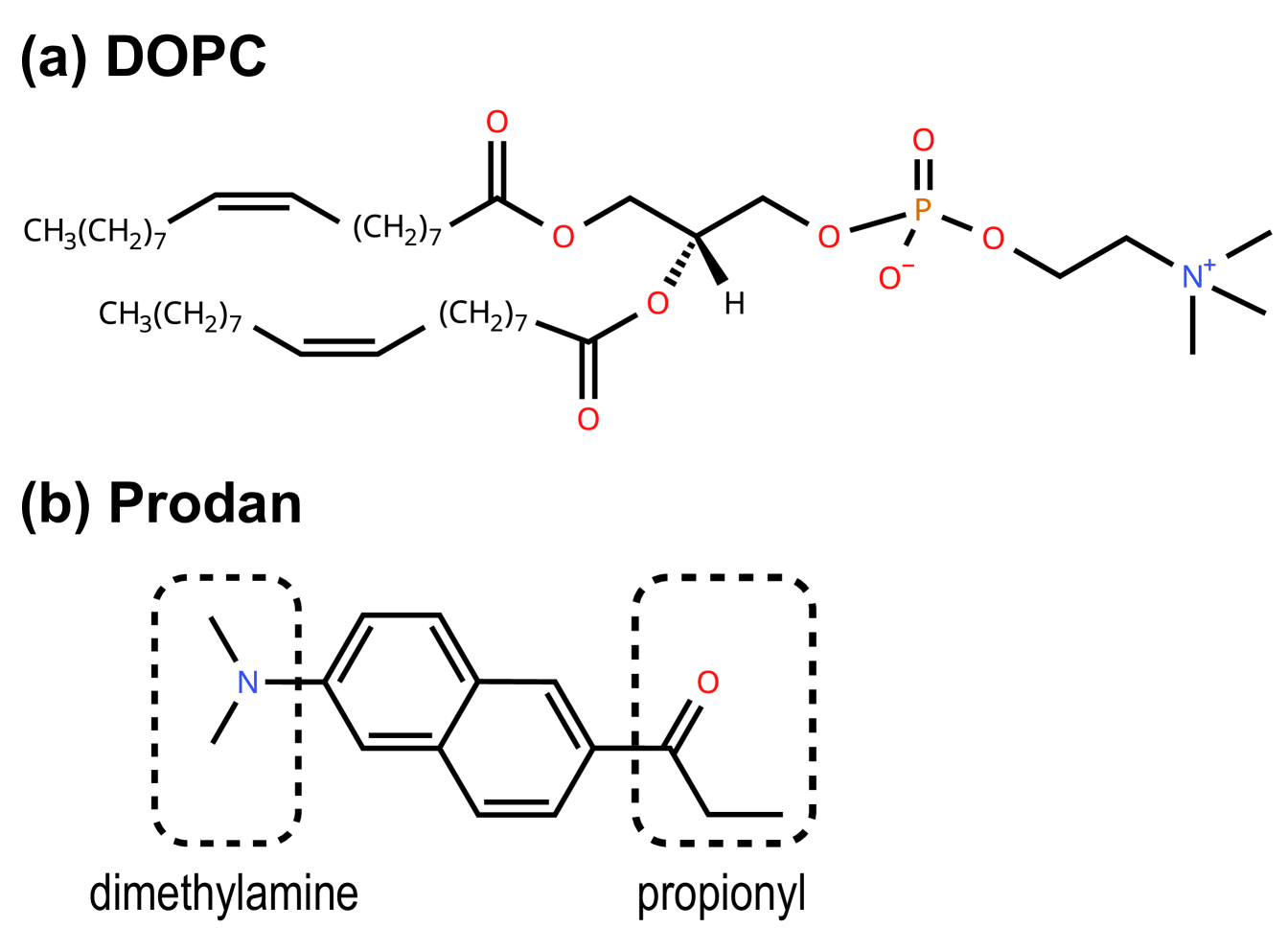
We investigated the membrane-probe systems composed of 1,2-dioleoyl-sn-glycero-3-phosphocholine (DOPC) lipid bilayer and a 6-propionyl-2-dimethylaminonaphthalene (Prodan) (Fig. 1). For the aqueous solutions facing the membrane, pure water, 1 M ethanol, and 2 M ethanol aqueous solutions were used. The force fields for DOPC, Prodan, ethanol, and water were CHARMM36,[52] CHARMM generalized force field (CGenFF),[53] CGenFF, and CHARMM-compatible TIP3P,[54] respectively. In this study, a pH of 7.0 is assumed, under which the dimethylamine group in Prodan is considered to be unprotonated (neutral), given that the $\mathrm{p}K_{\mathrm{a}}$ of the dimethylamine group is $\sim$ $4.5$ .[55] The electronic structure of Prodan was calculated using the CAM-B3LYP/cc-pVDZ level calculation.[56, 57] Then, the charges from electrostatic potentials using a grid based method (CHelpG) was used for calculating the point charges on the atoms in Prodan.[58] The above quantum chemical calculation was performed using Gaussian 16.[59] The target temperature and pressure were set to 310 K and 1 atm, respectively.

The initial configurations of the membrane were prepared using CHARMM-GUI server. [60, 61, 62] The number of DOPC molecules were 128 (64 per leaflet) for all the systems. The numbers of water and ethanol molecules, $\left(N_{\mathrm{wat}},N_{\mathrm{etoh}}\right)$ , were $\left(7680,0\right)$ for pure water, $\left(7250,140\right)$ for 1 M ethanol, and $\left(6910,280\right)$ for 2 M ethanol. The initial configurations of the aqueous phases were built using Packmol.[63]

All the MD simulations were performed with GENESIS 2.0.[64, 65, 66] We used the Bussi method for controlling the temperature and pressure.[67] For the initial equilibration stage, we performed MD simulations (1.875 ns in total; $NVT$ and $NPT$ ) using the velocity Verlet (VVER) integrator[68] with a time step of 2 fs, applying restraints to the membranes in accordance with the CHARMM-GUI guidelines. Subsequently, the reversible reference system propagator algorithm (r-RESPA) with a time interval of 2.5 fs was used for the simulations under $NPT$ condition. We conducted the 550 ns MD simulation for further equilibration. After the equilibration, we performed the REUS simulations with 32 replicas. In the REUS simulations, the reaction coordinate was defined as the $z$ -component of the center of mass (CoM) of Prodan, where the $z$ -direction is normal to the membrane surface and $z=0$ corresponds to the CoM of the membrane. Performing 30 ns MD simulations with automatic tuning of the REUS parameters,[69] the reference positions ${z_{i}}$ (corresponding to $\zeta_{i}$ in Eq. (1)) and the force constants ${k_{i}}$ were optimized (Tables S1–S4 of the supplementary material). After the 30 ns simulations without exchange, we conducted 500 ns REUS simulations for production. We also performed two independent 500 ns REUS simulations using the tuned parameters described above for estimating the statistical error. In these runs, 550 ns MD simulation was conducted for equilibration prior to the REUS simulations, starting from different initial configurations. The weights of the configurations in the REUS trajectories were computed by means of the MBAR method implemented in GENESIS.[70] The interaction energy analysis were performed using ERmod 0.3.7.[71]

To analyze the void existing inside the membrane, we performed the MD simulations for the membrane systems in the absence of Prodan. The initial configurations were prepared from those of the membrane-probe systems obtained after 550 ns equilibration mentioned above. After deleting the Prodan’s coordinates, the energy minimization was conducted. Then, we performed 100 ps NVT simulations using VVER, followed by 100 ns NPT simulations using r-RESPA. The last 50 ns were used for analysis.

Refer to caption — Figure 1: Chemical structures of (a) 1,2-dioleoyl-sn-glycero-3-phosphocholine (DOPC) and (b) 6-propionyl-2-dimethylaminonaphthalene (Prodan).

IV Results and discussion

IV.1 Free-energy landscapes

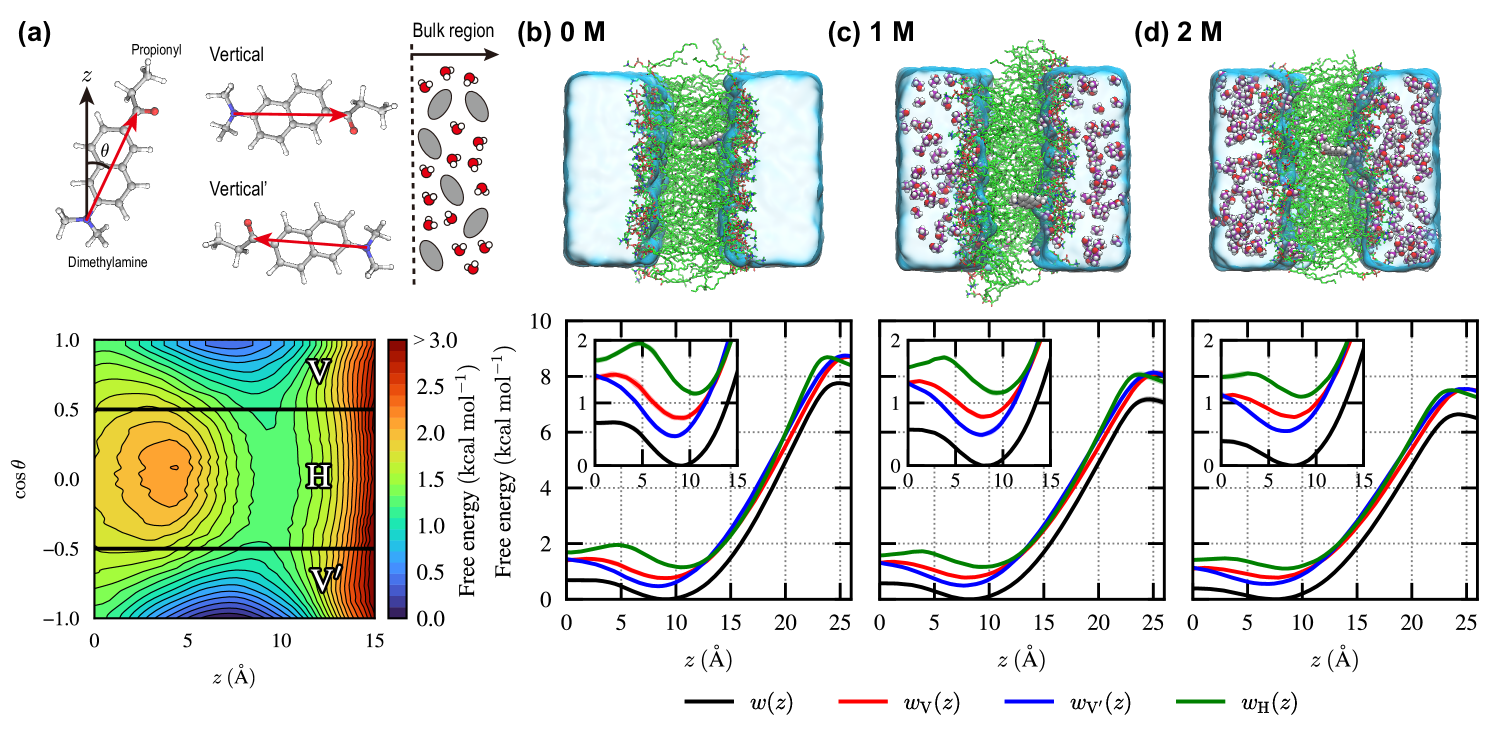
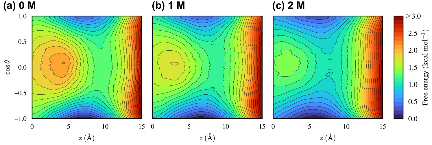
We first examine the two-dimensional free-energy landscape (2D-FEL) as a function of the $z$ -component of the center of mass (CoM) of Prodan, $z$ , and the cosine of the tilt angle, $\cos\theta$ (Fig. 2(a)). The tilt angle, $\theta$ , is defined as the angle between the membrane normal (the $z$ -direction) and the Prodan’s molecular axis pointing from the nitrogen atom in the dimethylamine group to the carbonyl carbon atom in the propionyl group. It can be seen from the 2D-FEL for the 0 M ethanol (pure water) case that stable embedded states appear around $z\sim 8~\mathrm{\AA }$ , with the molecular axis nearly parallel to the $z$ -direction ( $\cos\theta\sim\pm 1$ ). On the other hand, the inner region ( $z<4~\mathrm{\AA }$ ) is found to be unfavorable for Prodan especially when its molecular axis is oriented orthogonal to the $z$ -direction. Then, we define three regions based on $\cos\theta$ as follows: $\cos\theta>0.5$ , $\cos\theta<-0.5$ , and $-0.5\leq\cos\theta\leq 0.5$ are referred to as vertical ( $\mathrm{V}$ ), vertical’ ( $\mathrm{V}^{\prime}$ ), and horizontal ( $\mathrm{H}$ ), respectively. Since similar profiles are observed in the 2D-FELs for the 1 M and 2 M ethanol cases (Fig. S1 of the supplementary material), this definition is useful for analyzing how the thermodynamic stability of each region changes in the presence of ethanol.

To closely examine the change in thermodynamic stability for each region, we introduce the one-dimensional FELs (1D-FELs) with and without restriction to a specific region $\mathrm{X}$ ( $\mathrm{X}=\mathrm{V},\mathrm{V}^{\prime}$ , or $\mathrm{H}$ ), defined respectively as

	$\displaystyle w_{\mathrm{X}}\left(z\right)$	$\displaystyle=-\dfrac{1}{\beta}\log\dfrac{\Braket{\delta\left(z-z_{\mathrm{s}}\left(\bm{\Gamma}\right)\right)\Theta_{\mathrm{X}}\left(\cos\theta\right)}}{\Braket{\Theta_{\mathrm{X}}\left(\cos\theta\right)}}+C,$		(7)
	$\displaystyle w(z)$	$\displaystyle=-\dfrac{1}{\beta}\log\Braket{\delta\left(z-z_{\mathrm{s}}(\bm{\Gamma})\right)}+C,$		(8)

where $z_{\mathrm{s}}(\bm{\Gamma})$ is the $z$ -component of CoM of Prodan (solute) for a given phase-space coordinate $\bm{\Gamma}$ , and $\Theta_{\mathrm{X}}(\cos\theta)$ is the characteristic function that equals unity when $\cos\theta\in\mathrm{X}$ and zero otherwise. $C$ is the normalization constant, which is determined such that the lowest value of $w\left(z\right)$ is zero. Fig. 2(b)–(d) illustrate the 1D-FELs for the 0, 1, and 2 M ethanol cases, respectively. For all the cases, region $\mathrm{V}^{\prime}$ exhibits the most stable state at $\sim$ $8~\mathrm{\AA }$ . It is interesting to note that region $\mathrm{V}^{\prime}$ is more stable than region $\mathrm{V}$ , despite the stabilization effect from the electrostatic interaction between Prodan and the aqueous phase being weaker in region $\mathrm{V}^{\prime}$ than in region $\mathrm{V}$ due to the increased distance between the propionyl group and the aqueous phase in region $\mathrm{V}^{\prime}$ (Fig. 2(a)). Region $\mathrm{H}$ at the corresponding $z$ is found to be unstable compared with regions $\mathrm{V}$ and $\mathrm{V}^{\prime}$ , as is also seen in the 2D-FEL (Fig. 2(a)). As the ethanol concentration increases, the difference in thermodynamic stability among the different regions at $z\leq 15~\mathrm{\AA }$ becomes smaller, indicating that the extent of the orientation preference is mitigated by adding ethanol. Regarding the interface ( $z\sim 20-25~\mathrm{\AA }$ ), a high free-energy barrier is present, reflecting the hydrophobic nature of Prodan, and the difference in the barrier height between different regions is negligibly small. In the presence of ethanol, it is observed that the barrier height is lowered. This trend is consistent with experimental observations that ethanol acts as a permeation enhancer.[6, 7]

IV.2 Decomposition of free energy

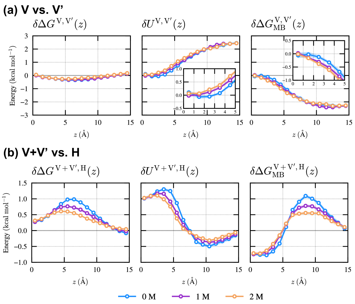
In this subsection, we discuss the change in the stability of each state due to the addition of ethanol in terms of the systematic decomposition of free energy according to the classical density functional theory. The free-energy difference between regions $\mathrm{X}_{0}$ and $\mathrm{X}_{1}$ , $\delta\Delta G^{\mathrm{X_{0},X_{1}}}\left(z\right)$ , given by

\displaystyle\delta\Delta G^{\mathrm{X_{0},X_{1}}}\left(z\right)

\displaystyle=-\dfrac{1}{\beta}\log\dfrac{\Braket{\Theta_{\mathrm{X_{1}}}\left(\cos\theta\right)\delta\left(z-z_{\mathrm{s}}\left(\bm{\Gamma}\right)\right)}}{\Braket{\Theta_{\mathrm{X_{0}}}\left(\cos\theta\right)\delta\left(z-z_{\mathrm{s}}\left(\bm{\Gamma}\right)\right)}},

(9)

can be decomposed into the difference in the interaction energy of Prodan with the surrounding environment, $\delta U^{\mathrm{X_{0},X_{1}}}\left(z\right)$ , and the many-body entropic contribution, $\delta\Delta G_{\mathrm{MB}}^{\mathrm{X}_{0},\mathrm{X}_{1}}\left(z\right)$ , as

\displaystyle\delta\Delta G^{\mathrm{X_{0},X_{1}}}\left(z\right)

\displaystyle=\delta U^{\mathrm{X_{0},X_{1}}}\left(z\right)+\delta\Delta G_{\mathrm{MB}}^{\mathrm{X_{0},X_{1}}}\left(z\right).

(10)

$\delta\Delta G_{\mathrm{MB}}^{\mathrm{X}_{0},\mathrm{X}_{1}}\left(z\right)$ is the difference in the free-energy penalty due to the distortion of the surrounding environment upon the insertion of Prodan between regions $\mathrm{X}_{0}$ and $\mathrm{X}_{1}$ .

Fig. 3(a) shows the free-energy difference between regions $\mathrm{V}$ and $\mathrm{V}^{\prime}$ , denoted as $\delta\Delta G^{\mathrm{V},\mathrm{V}^{\prime}}\left(z\right)$ , together with its decomposition. It is observed that the slightly higher stability of region $\mathrm{V}^{\prime}$ compared to region $\mathrm{V}$ stems from a more negative value of $\delta\Delta G_{\mathrm{MB}}^{\mathrm{V},\mathrm{V}^{\prime}}$ , suggesting that the extent of membrane distortion upon Prodan insertion is smaller in region $\mathrm{V}^{\prime}$ than in region $\mathrm{V}$ , especially when Prodan is distant from the membrane center. The positive value of $\delta U^{\mathrm{V,V^{\prime}}}\left(z\right)$ indicates that the stabilization effect of the interaction between Prodan and its surrounding environment is stronger in region $\mathrm{V}$ than in region $\mathrm{V}^{\prime}$ , although the magnitude of $\delta U^{\mathrm{V,V^{\prime}}}\left(z\right)$ is smaller than that of $\delta\Delta G_{\mathrm{MB}}^{\mathrm{V,V^{\prime}}}\left(z\right)$ . As the ethanol concentration increases, the stability of region $\mathrm{V}^{\prime}$ relative to region $\mathrm{V}$ slightly decreases due to an increase in $\delta U^{\mathrm{V},\mathrm{V}^{\prime}}\left(z\right)$ .

The stability of region $\mathrm{H}$ is lower than that of the composite region of $\mathrm{V}$ and $\mathrm{V}^{\prime}$ , $\mathrm{V}+\mathrm{V}^{\prime}$ , for the 0 M ethanol case, as indicated by $\delta\Delta G^{\mathrm{V}+\mathrm{V}^{\prime},\mathrm{H}}\left(z\right)$ (Fig. 3(b)), especially at $z\sim$ $6~\mathrm{\AA }$ . Interestingly, the decomposition of $\Delta G^{\mathrm{V+V^{\prime},H}}\left(z\right)$ reveals that the factors contributing to the stabilization or destabilization of region H with respect to region $\mathrm{V+V^{\prime}}$ vary depending on the $z$ -range. The destabilizing effect of $\delta U^{\mathrm{V+V^{\prime},H}}\left(z\right)$ is evident for $z\lesssim 7.5~\mathrm{\AA }$ and reaches its maximum around $z\sim$ $4~\mathrm{\AA }$ , resulting in the most unstable state in region $\mathrm{H}$ at $z\sim$ $6~\mathrm{\AA }$ . It is seen that $\delta\Delta G_{\mathrm{MB}}^{\mathrm{V+V^{\prime},H}}\left(z\right)$ contributes to the stabilization for $z\lesssim 5~\mathrm{\AA }$ and its magnitude is smaller than that of $\delta U^{\mathrm{V+V^{\prime},H}}\left(z\right)$ . $\Delta G_{\mathrm{MB}}^{\mathrm{V+V^{\prime},H}}\left(z\right)$ , in turn, significantly destabilizes region $\mathrm{H}$ around $z\sim$ $8~\mathrm{\AA }$ . In the presence of ethanol, region H is found to be stabilized due to the reduction in the destabilizing effects of $\delta U^{\mathrm{V+V^{\prime},H}}\left(z\right)$ and $\delta\Delta G_{\mathrm{MB}}^{\mathrm{V+V^{\prime},H}}\left(z\right)$ .

IV.3 Void-size distribution along $z$ -direction

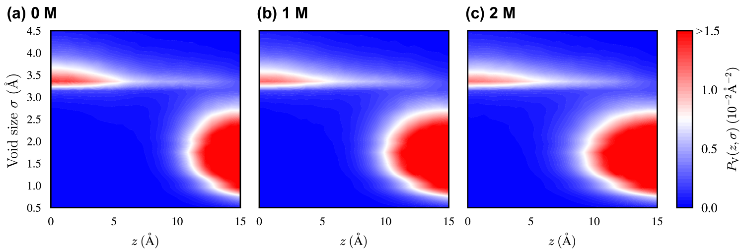
We discuss the structural property of the membrane. According to previous simulation studies on membrane permeation, [72, 73, 74] voids, defined as spaces not occupied by atoms, exist within the membrane, particularly near its center. Such voids can reduce the free-energy penalty due to the distortion of the membrane caused by the embedding of molecules that are related with $\delta\Delta G^{\mathrm{X}_{0},\mathrm{X}_{1}}_{\mathrm{MB}}$ . Therefore, quantifying these voids is essential for elucidating the embedded states. In this work, we compute the distribution of the void size ( $\sigma$ ) along the $z$ -direction, $P_{\mathrm{V}}\left(z,\sigma\right)$ , based on an algorithm developed in the field of computational material science (Appendix A).[75] The trajectory in the absence of Prodan is used for computing $P_{\mathrm{V}}\left(z,\sigma\right)$ .

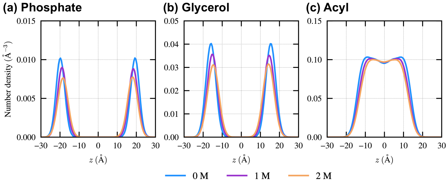
Fig. 4 shows the $P_{\mathrm{V}}\left(z,\sigma\right)$ for the 0, 1, and 2 M ethanol cases. In all cases, large voids ( $\sigma\geq 3~\mathrm{\AA }$ ) are populated near the membrane center. This observation is consistent with the previous studies.[73, 74] Such large voids can accommodate bulky molecules or moieties with a low free-energy penalty. Thus, the stabilizing effect of the voids on region $\mathrm{H}$ is pronounced for the many-body entropic term when Prodan is located near the membrane center, as all of its atoms are embedded within the membrane center. A broad distribution of $\sigma$ is observed around $z=12-15\mathrm{\AA }$ , where the glycerol groups of DOPC molecules are located (Fig. S2 of the supplementary material). Since the length of Prodan along its molecular axis is $\sim$ $10~\mathrm{\AA }$ , the presence of voids near the membrane center and $z=12-15~\mathrm{\AA }$ is expected to facilitate the preferential embedding of Prodan in regions $\mathrm{V}$ and $\mathrm{V}^{\prime}$ , rather than in region $\mathrm{H}$ , when Prodan’s CoM is located within $z=8-10~\mathrm{\AA }$ . In the presence of ethanol, a decrease in the population of large voids near the membrane center is observed, while the overall shape of $P_{\mathrm{V}}\left(z,\sigma\right)$ remains largely changed. This reduction may account for the decreased difference in stability between regions $\mathrm{V+V^{\prime}}$ and $\mathrm{H}$ , as reflected by the decrease in $\Delta G^{\mathrm{V+V^{\prime}},\mathrm{H}}_{\mathrm{MB}}$ (Fig. 3(b)).

IV.4 Electrostatic interaction of Prodan with surrounding environments

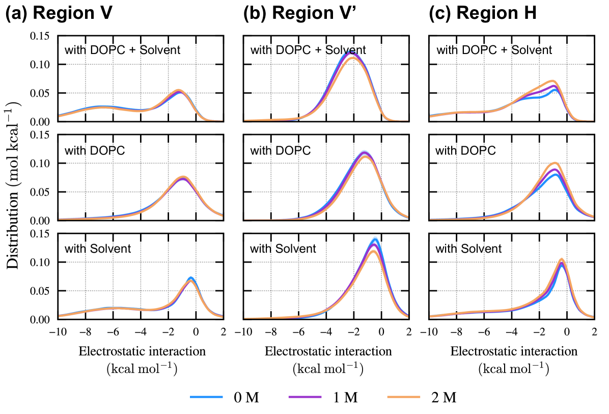
The electrostatic interactions between Prodan and its surrounding environments are elucidated in this subsection. Given that the electrostatic interactions dominantly contribute to the excitation properties, analyzing the interaction patterns is beneficial for discussing the connection between the embedded state and the excitation behavior.

In Fig. 5, the distributions of the electrostatic interaction for different embedded states, $\mathrm{V}$ , $\mathrm{V}^{\prime}$ , and $\mathrm{H}$ , are illustrated. The distributions are calculated from snapshots in which the CoM of Prodan is located closer to the membrane center than the average position of the phosphorus atoms in the DOPC molecules. For region $\mathrm{V}$ (Fig. 5(a)), there are two peaks at $\sim$ $-7~\mathrm{kcal~mol^{-1}}$ and $\sim$ $-1~\mathrm{kcal~mol^{-1}}$ , and the shape of the distribution is hardly changed upon the addition of ethanol. As revealed by the decomposition into contributions from DOPC and solvent (water and ethanol), the peak at $\sim$ $-7~\mathrm{kcal~mol^{-1}}$ originates from the solvent. Since the propionyl moiety is oriented toward the membrane–solvent interface in region $\mathrm{V}$ and can strongly interact with the solvent, it is reasonable that the solvent contributes to this peak. It can be seen that the peak at $\sim$ $-1~\mathrm{kcal~mol^{-1}}$ stems from both the DOPC and solvent. Regarding region $\mathrm{V}^{\prime}$ (Fig. 5(b)), only a broad distribution centered at $\sim$ $-2~\mathrm{kcal~mol^{-1}}$ is observed. Since the dimethylamine group is located near the membrane-solvent surface in region $\mathrm{V}^{\prime}$ , the absence of the peak observed at the more negative value in region $\mathrm{V}$ reflects the lower hydrophilicity of the dimethylamine group compared with the propionyl group. As the ethanol concentration increases, the peak of the interaction with DOPC and solvent shifts in a positive direction. This shift is caused by the slight weakening of the interaction with DOPC. As shown in Fig. 5(c), region $\mathrm{H}$ exhibits a distribution in which the interaction with DOPC and solvent is more negative than $-6~\mathrm{kcal~mol^{-1}}$ , similar to region $\mathrm{V}$ . Adding ethanol increases the population around $\sim$ $–1~\mathrm{kcal~mol^{-1}}$ , and this change clearly originates from DOPC.

V Conclusion

In this study, we investigated the embedding of Prodan within a lipid bilayer composed of 1,2-dioleoyl-sn-glycero-3-phosphocholine (DOPC) using the molecular dynamics (MD) simulation with the replica-exchange umbrella sampling (REUS) method. Employing the REUS method enables the evaluation of free-energy landscapes (FELs) for the embedded state with high statistical reliability. The response of the embedded states to the addition of ethanol as a cosolvent in the aqueous phase was also examined, given that ethanol is known to distort membrane structures.

The two-dimensional free-energy landscapes (2D-FELs) along the $z$ -component of the center of mass (CoM) of Prodan and its orientation identified two stable regions within the membrane, in which the propionyl and dimethylamine groups of Prodan are respectively directed toward the aqueous phase. These regions were referred to as $\mathrm{V}$ and $\mathrm{V}^{\prime}$ , respectively, while the less stable region in which the molecular axis of Prodan is oriented perpendicular to the $z$ -direction (normal to the membrane surface) was denoted as $\mathrm{H}$ . The stabilities of regions $\mathrm{V}$ and $\mathrm{V}^{\prime}$ were similar, with $\mathrm{V}^{\prime}$ being slightly more stable. The one-dimensional FELs (1D-FELs), restricted to a specific region, revealed that the orientational preferences in regions $\mathrm{V}$ and $\mathrm{V}^{\prime}$ are mitigated by the addition of ethanol to the aqueous phase. The exact decomposition of the FELs into the interaction energy of Prodan with its surrounding environment and the many-body entropic contribution showed that the comparable stability of regions $\mathrm{V}$ and $\mathrm{V}^{\prime}$ arises from a balance between stabilizing effects from the interaction energy contribution and destabilizing effects from the entropic contribution. The instability of region $\mathrm{H}$ , compared with the composite region of regions $\mathrm{V}$ and $\mathrm{V}^{\prime}$ , $\mathrm{V+V^{\prime}}$ , originated from the interaction energy near the membrane center and from the entropic contribution around $z\sim$ $8~\mathrm{\AA }$ . The stability difference between region $\mathrm{H}$ and $\mathrm{V+V^{\prime}}$ decreased upon the addition of ethanol, due to reduced differences in both the interaction-energy and the entropic contributions. Furthermore, the void-size distributions within the membrane suggest that the reduced destabilizing effects from the entropic contribution are correlated with a decrease in large voids near the membrane center. Such large voids can accommodate bulky molecules or moieties, so their reduction may lead to the relative destabilization of region $\mathrm{V+V^{\prime}}$ when Prodan is located within $z=8-10~\mathrm{\AA }$ , thereby reducing the stability difference. The electrostatic interaction of Prodan with its surrounding environment was stronger in the order $\mathrm{V}^{\prime}>\mathrm{H}>\mathrm{V}$ , a trend primarily determined by its interaction with the solvent.

To further investigate a probe within membranes, incorporating a theoretical treatment of its electronic structure is an important step. Practically, the quantum mechanics/molecular mechanics (QM/MM) method is a useful approach for studying excitation properties in heterogeneous environments such as membranes. Osella et al.[76] and Wasif et al.[34] applied this method to investigate the excitation of probes within membranes, successfully characterizing their spectra. Recent advances in computing power and molecular dynamics (MD) software[77] have made it possible to combine QM/MM simulations with the REUS method for large-scale systems. Thus, employing such a technique could allow for a more realistic description of the embedded states. Investigating the effects of different protonation states of Prodan on its embedded states is another imporant step, especially when the target membrane is associated with the gastrointestinal environment, where the pH ranges from 1.5 to 8. The $\mathrm{p}K_{\mathrm{a}}$ of the dimethylamine group in Prodan is $\sim$ $4.5$ , and hence its predominant protonation state varies across different regions of the gastrointestinal membrane. Constant-pH MD methods,[78, 79, 80, 81, 82, 83] which enable us to treat multiple protonation states, would be useful for analyzing the embedded states of probes within membranes that mimic the gastrointestinal environment. Further elucidation using the aforementioned sophisticated techniques would deepen our understanding of membrane properties through a more detailed interpretation of the spectra.

Supplementary Material

The supplementary material contains the initial and optimized parameters for the restraint potentials used in the REUS simulations, the free-energy landscapes of Prodan along the $z$ -component of the center of mass (CoM) for Prodan, $z$ , and the cosine of the tilt angle, $\cos\theta$ , and the distributions along the $z$ -direction of atoms in phosphate group, glycerol group, and acyl chains.

Acknowledgements.

This work is supported by the Grants-in-Aid for Scientific Research (Nos. JP21H05249, JP23K27313, JP23K26617, JP25KJ1759, and JP25K17896) from the Japan Society for the Promotion of Science, the Fugaku Supercomputer Project (Nos. JPMXP1020230325 and JPMXP1020230327) and the Data-Driven Material Research Project (No. JPMXP1122714694) from the Ministry of Education, Culture, Sports, Science, and Technology, the Core Research for Evolutional Science and Technology (CREST) from Japan Science and Technology Agency (JST) (No. JPMJCR22E3), and by Maruho Collaborative Project for Theoretical Pharmaceutics. The simulations were conducted using Genkai A at Kyushu University, and Fugaku at RIKEN Center for Computational Science through the HPCI System Research Project (Project IDs: hp250115, hp250211, hp250227, and hp250229).

Conflict of interest

The authors have no conflicts to disclose.

Data Availability

The data that support the findings of this study are available from the corresponding authors upon reasonable request.

Appendix A Definition of void-size distribution $P_{\mathrm{V}}\left(z,\sigma\right)$

To analyze the distribution of voids within the membrane, defined as regions not occupied by atoms in the system, we employ a numerical technique for estimating void size, developed in the field of mesoporous material science.[75] The voids referred to here are called “pores” in that field. However, since “voids” is the term used in a recent membrane simulation study,[74] we adopt it in this work.

Let $d_{\mathrm{V},\lambda}\left(z\right)$ denote the size of the $\lambda$ th void whose center, ${\bf x}_{\lambda}$ , lies between $z$ and $z+\Delta z$ . We suppose that all the voids located within this interval satisfy the following conditions.

	$\displaystyle\forall\lambda\leq N_{\mathrm{V}}\left(z\right)\quad d_{\mathrm{V},\lambda}\left(z\right)=2\min_{i}\left(\left\|{\bf x}_{\lambda}-{\bf r}_{i}\right\|-\dfrac{\sigma_{i}}{2}\right),$		(11)
	$\displaystyle\forall\lambda,\mu\leq N_{\mathrm{V}}\left(z\right),\lambda\neq\mu\quad\left\|\mathbf{x}_{\lambda}-\mathbf{x}_{\mu}\right\|>\dfrac{1}{2}d_{\mathrm{V},\mu}(z).$		(12)
	$\displaystyle\forall\lambda\leq N_{\mathrm{V}}\left(z\right),\forall i\leq N_{\mathrm{atom}}\quad\left\|{\bf x}_{\lambda}-{\bf r}_{i}\right\|>\dfrac{\sigma_{i}}{2}.$		(13)

Here, ${\bf r}_{i}$ is the position of $i$ th atom in the system, and $\sigma_{i}$ is its diameter. $N_{\mathrm{V}}\left(z\right)$ is the number of voids whose centers are located between $z$ and $z+\Delta z$ , and $N_{\mathrm{atom}}$ is the number of atoms in the system. $d_{\mathrm{V},\lambda}\left(z\right)$ represents the maximum diameter of the sphere centered at ${\bf x}_{\lambda}$ that does not contain any atoms. Eqs. (12) and (13) ensure that no void contains the center of any other void, and that all void centers are located outside the atoms in the system, respectively. Then, let us define the unnormalized void density as

\displaystyle\rho_{\mathrm{V}}\left(z,\sigma\right)

\displaystyle=\Braket{\dfrac{1}{\Delta z}\sumop_{i=1}^{N_{\mathrm{V}}\left(z\right)}\delta\left(\sigma-d_{\mathrm{V},i}\left(z\right)\right)}.

(14)

Normalization is introduced as

\displaystyle P_{\mathrm{V}}\left(z,\sigma\right)

\displaystyle=\rho_{\mathrm{V}}\left(z,\sigma\right)\left({\displaystyle\intop\nolimits_{0}^{\mathrm{z_{\mathrm{P}}}}dz\intop\nolimits_{0}^{\infty}d\sigma}\,\rho_{\mathrm{V}}\left(z,\sigma\right)\right)^{-1}.

(15)

Here, $z_{\mathrm{P}}$ is the average $z$ -coordinate of the phosphorus atoms in DOPC molecules, measured from the membrane center ( $z=0$ ).

The code for computing $P_{\mathrm{V}}\left(z\right)$ is implemented in PoreBlazer v4.0.[75] We use $\sigma$ parameters of the Lennard-Jones interaction in the CHARMM36 force field[52].

References

Yeagle [2004] P. L. Yeagle, The structure of biological membranes (CRC press, 2004).
Komizu et al. [2011] Y. Komizu, S. Nakata, K. Goto, Y. Matsumoto, and R. Ueoka, “Membrane-targeted nanotherapy with hybrid liposomes for tumor cells leading to apoptosis,” ACS Med. Chem. Lett. 2, 275–279 (2011).
Liu, Testa, and Fahr [2011] X. Liu, B. Testa, and A. Fahr, “Lipophilicity and its relationship with passive drug permeation,” Pharm. Res. 28, 962–977 (2011).
Goldstein [1984] D. B. Goldstein, “The effects of drugs on membrane fluidity.” Annu. Rev. Pharmacol. Toxicol. 24, 43–64 (1984).
López et al. [2021] R. R. López, P. G. F. de Rubinat, L.-M. Sánchez, T. Tsering, A. Alazzam, K.-F. Bergeron, C. Mounier, J. V. Burnier, I. Stiharu, and V. Nerguizian, “The effect of different organic solvents in liposome properties produced in a periodic disturbance mixer: Transcutol®, a potential organic solvent replacement,” Colloids Surf. B Biointerfaces 198, 111447 (2021).
Pershing, Lambert, and Knutson [1990] L. K. Pershing, L. D. Lambert, and K. Knutson, “Mechanism of ethanol-enhanced estradiol permeation across human skin in vivo,” Pharm. Res. 7, 170–175 (1990).
Rai et al. [2024] R. Rai, D. Kumar, A. A. Dhule, B. A. Rudani, and S. Tiwari, “Alkanols regulate the fluidity of phospholipid bilayer in accordance to their concentration and polarity,” Langmuir 40, 14057–14065 (2024).
Lakowicz [2006] J. R. Lakowicz, Principles of fluorescence spectroscopy (Springer, 2006).
Demchenko et al. [2009] A. P. Demchenko, Y. Mély, G. Duportail, and A. S. Klymchenko, “Monitoring biophysical properties of lipid membranes by environment-sensitive fluorescent probes,” Biophys. J. 96, 3461–3470 (2009).
Gunther et al. [2021] G. Gunther, L. Malacrida, D. M. Jameson, E. Gratton, and S. A. Sánchez, “Laurdan since weber: the quest for visualizing membrane heterogeneity,” Acc. Chem. Res. 54, 976–987 (2021).
Krasnowska, Gratton, and Parasassi [1998] E. K. Krasnowska, E. Gratton, and T. Parasassi, “Prodan as a membrane surface fluorescence probe: partitioning between water and phospholipid phases,” Biophys. J. 74, 1984–1993 (1998).
Jurkiewicz et al. [2006] P. Jurkiewicz, A. Olżyńska, M. Langner, and M. Hof, “Headgroup hydration and mobility of dotap/dopc bilayers: a fluorescence solvent relaxation study,” Langmuir 22, 8741–8749 (2006).
Weber and Farris [1979] G. Weber and F. J. Farris, “Synthesis and spectral properties of a hydrophobic fluorescent probe: 6-propionyl-2-(dimethylamino) naphthalene,” Biochemistry 18, 3075–3078 (1979).
Macgregor and Weber [1986] R. B. Macgregor and G. Weber, “Estimation of the polarity of the protein interior by optical spectroscopy,” Nature 319, 70–73 (1986).
Massey and Pownall [1998] J. B. Massey and H. J. Pownall, “Surface properties of native human plasma lipoproteins and lipoprotein models,” Biophys. J. 74, 869–878 (1998).
Krasnowska et al. [2001] E. K. Krasnowska, L. A. Bagatolli, E. Gratton, and T. Parasassi, “Surface properties of cholesterol-containing membranes detected by prodan fluorescence,” Biochim. Biophys. Acta - Biomembr. 1511, 330–340 (2001).
Parasassi et al. [1991] T. Parasassi, G. De Stasio, G. Ravagnan, R. Rusch, and E. Gratton, “Quantitation of lipid phases in phospholipid vesicles by the generalized polarization of laurdan fluorescence,” Biophys. J. 60, 179–189 (1991).
Parasassi et al. [1995] T. Parasassi, A. M. Giusti, M. Raimondi, and E. Gratton, “Abrupt modifications of phospholipid bilayer properties at critical cholesterol concentrations,” Biophys. J. 68, 1895–1902 (1995).
Parasassi and Gratton [1995] T. Parasassi and E. Gratton, “Membrane lipid domains and dynamics as detected by laurdan fluorescence,” J. Fluoresc. 5, 59–69 (1995).
Parasassi et al. [1998] T. Parasassi, E. K. Krasnowska, L. Bagatolli, and E. Gratton, “Laurdan and prodan as polarity-sensitive fluorescent membrane probes,” J. Fluoresc. 8, 365–373 (1998).
Ito et al. [2023] N. Ito, N. M. Watanabe, Y. Okamoto, and H. Umakoshi, “Multiplicity of solvent environments in lipid bilayer revealed by das deconvolution of twin probes: Comparative method of laurdan and prodan,” Biophys. J. 122, 4614–4623 (2023).
Ito et al. [2024] N. Ito, N. M. Watanabe, Y. Okamoto, and H. Umakoshi, “Multifocal lipid membrane characterization by combination of das-deconvolution and anisotropy,” Biophys. J. 123, 4135–4146 (2024).
Allen and Tildesley [1989] M. P. Allen and D. J. Tildesley, Computer simulation of liquids (Oxford university press, 1989).
Frenkel and Smit [2001] D. Frenkel and B. Smit, Understanding molecular simulation: from algorithms to applications, Vol. 1 (Elsevier, 2001).
Jurkiewicz et al. [2012] P. Jurkiewicz, L. Cwiklik, P. Jungwirth, and M. Hof, “Lipid hydration and mobility: an interplay between fluorescence solvent relaxation experiments and molecular dynamics simulations,” Biochimie 94, 26–32 (2012).
Moradi, Nowroozi, and Shahlaei [2019] S. Moradi, A. Nowroozi, and M. Shahlaei, “Shedding light on the structural properties of lipid bilayers using molecular dynamics simulation: a review study,” RSC Adv. 9, 4644–4658 (2019).
Hsieh, Yu, and Klauda [2021] M.-K. Hsieh, Y. Yu, and J. B. Klauda, “All-atom modeling of complex cellular membranes,” Langmuir 38, 3–17 (2021).
Majumder et al. [2024] A. Majumder, Y. Gu, Y.-C. Chen, X. An, B. M. Reinhard, and J. E. Straub, “Probing the origins of the disorder-to-order transition of a modified cholesterol in ternary lipid bilayers,” J. Am. Chem. Soc. 146, 27725–27735 (2024).
Cwiklik et al. [2011] L. Cwiklik, A. J. Aquino, M. Vazdar, P. Jurkiewicz, J. Pittner, M. Hof, and H. Lischka, “Absorption and fluorescence of prodan in phospholipid bilayers: A combined quantum mechanics and classical molecular dynamics study,” J. Phys. Chem. A 115, 11428–11437 (2011).
Nitschke et al. [2012] W. K. Nitschke, C. C. Vequi-Suplicy, K. Coutinho, and H. Stassen, “Molecular dynamics investigations of prodan in a dlpc bilayer,” J. Phys. Chem. B 116, 2713–2721 (2012).
Suhaj et al. [2018] A. Suhaj, A. Le Marois, D. J. Williamson, K. Suhling, C. D. Lorenz, and D. M. Owen, “Prodan differentially influences its local environment,” Phys. Chem. Chem. Phys. 20, 16060–16066 (2018).
Suhaj et al. [2020] A. Suhaj, D. Gowland, N. Bonini, D. M. Owen, and C. D. Lorenz, “Laurdan and di-4-aneppdhq influence the properties of lipid membranes: A classical molecular dynamics and fluorescence study,” J. Phys. Chem. B (2020).
Osella et al. [2016a] S. Osella, N. A. Murugan, N. K. Jena, and S. Knippenberg, “Investigation into biological environments through (non) linear optics: A multiscale study of laurdan derivatives,” J. Chem. Theory Comput. 12, 6169–6181 (2016a).
Wasif Baig et al. [2018] M. Wasif Baig, M. Pederzoli, P. Jurkiewicz, L. Cwiklik, and J. Pittner, “Orientation of laurdan in phospholipid bilayers influences its fluorescence: Quantum mechanics and classical molecular dynamics study,” Molecules 23, 1707 (2018).
Osella and Knippenberg [2021] S. Osella and S. Knippenberg, “The influence of lipid membranes on fluorescent probes’ optical properties,” Biochim. Biophys. Acta - Biomembr. 1863, 183494 (2021).
Knippenberg et al. [2024] S. Knippenberg, K. De, C. Aisenbrey, B. Bechinger, and S. Osella, “Hydration-and temperature-dependent fluorescence spectra of laurdan conformers in a dppc membrane,” Cells 13, 1232 (2024).
Sugita and Okamoto [1999] Y. Sugita and Y. Okamoto, “Replica-exchange molecular dynamics method for protein folding,” Chem. Phys. Lett. 314, 141–151 (1999).
Sugita, Kitao, and Okamoto [2000] Y. Sugita, A. Kitao, and Y. Okamoto, “Multidimensional replica-exchange method for free-energy calculations,” J. Chem. Phys. 113, 6042–6051 (2000).
Murata, Sugita, and Okamoto [2004] K. Murata, Y. Sugita, and Y. Okamoto, “Free energy calculations for dna base stacking by replica-exchange umbrella sampling,” Chem. Phys. Lett. 385, 1–7 (2004).
Venable, Krämer, and Pastor [2019] R. M. Venable, A. Krämer, and R. W. Pastor, “Molecular dynamics simulations of membrane permeability,” Chem. Rev. 119, 5954–5997 (2019).
Bemporad, Essex, and Luttmann [2004] D. Bemporad, J. W. Essex, and C. Luttmann, “Permeation of small molecules through a lipid bilayer: a computer simulation study,” J. Phys. Chem. B 108, 4875–4884 (2004).
Ghaemi et al. [2012] Z. Ghaemi, M. Minozzi, P. Carloni, and A. Laio, “A novel approach to the investigation of passive molecular permeation through lipid bilayers from atomistic simulations,” J. Phys. Chem. B 116, 8714–8721 (2012).
Lee et al. [2016] C. T. Lee, J. Comer, C. Herndon, N. Leung, A. Pavlova, R. V. Swift, C. Tung, C. N. Rowley, R. E. Amaro, C. Chipot, et al., “Simulation-based approaches for determining membrane permeability of small compounds,” J. Chem. Inf. Model. 56, 721–733 (2016).
Cipcigan et al. [2020] F. Cipcigan, P. Smith, J. Crain, A. Hogner, L. De Maria, A. Llinas, and E. Ratkova, “Membrane permeability in cyclic peptides is modulated by core conformations,” J. Chem. Inf. Model. 61, 263–269 (2020).
Sugita et al. [2021] M. Sugita, S. Sugiyama, T. Fujie, Y. Yoshikawa, K. Yanagisawa, M. Ohue, and Y. Akiyama, “Large-scale membrane permeability prediction of cyclic peptides crossing a lipid bilayer based on enhanced sampling molecular dynamics simulations,” J. Chem. Inf. Model. 61, 3681–3695 (2021).
Matsubara et al. [2024] Y. Matsubara, R. Okabe, R. Masayama, N. M. Watanabe, H. Umakoshi, K. Kasahara, and N. Matubayasi, “A methodology of quantifying membrane permeability based on returning probability theory and molecular dynamics simulation,” arXiv preprint arXiv:2404.11363 (2024).
Gurtovenko and Anwar [2009] A. A. Gurtovenko and J. Anwar, “Interaction of ethanol with biological membranes: the formation of non-bilayer structures within the membrane interior and their significance,” J. Phys. Chem. B 113, 1983–1992 (2009).
Barry and Gawrisch [1995] J. A. Barry and K. Gawrisch, “Effects of ethanol on lipid bilayers containing cholesterol, gangliosides, and sphingomyelin,” Biochemistry 34, 8852–8860 (1995).
Rottenberg [1992] H. Rottenberg, “Probing the interactions of alcohols with biological membranes with the fluorescent probe prodan,” Biochemistry 31, 9473–9481 (1992).
Zeng and Chong [1995] J. Zeng and P. Chong, “Effect of ethanol-induced lipid interdigitation on the membrane solubility of prodan, acdan, and laurdan,” Biophys. J. 68, 567–573 (1995).
Shirts and Chodera [2008] M. R. Shirts and J. D. Chodera, “Statistically optimal analysis of samples from multiple equilibrium states,” J. Chem. Phys. 129 (2008).
Klauda et al. [2010] J. B. Klauda, R. M. Venable, J. A. Freites, J. W. O’Connor, D. J. Tobias, C. Mondragon-Ramirez, I. Vorobyov, A. D. MacKerell Jr, and R. W. Pastor, “Update of the charmm all-atom additive force field for lipids: validation on six lipid types,” J. Phys. Chem. B 114, 7830–7843 (2010).
Vanommeslaeghe et al. [2010] K. Vanommeslaeghe, E. Hatcher, C. Acharya, S. Kundu, S. Zhong, J. Shim, E. Darian, O. Guvench, P. Lopes, I. Vorobyov, et al., “Charmm general force field: A force field for drug-like molecules compatible with the charmm all-atom additive biological force fields,” J. Comput. Chem. 31, 671–690 (2010).
Jorgensen et al. [1983] W. L. Jorgensen, J. Chandrasekhar, J. D. Madura, R. W. Impey, and M. L. Klein, “Comparison of simple potential functions for simulating liquid water,” J. Chem. Phys. 79, 926–935 (1983).
Chong, Capes, and Wong [1989] P. L. G. Chong, S. Capes, and P. T. Wong, “Effects of hydrostatic pressure on the location of prodan in lipid bilayers: a ft-ir study,” Biochemistry 28, 8358–8363 (1989).
Yanai, Tew, and Handy [2004] T. Yanai, D. P. Tew, and N. C. Handy, “A new hybrid exchange–correlation functional using the coulomb-attenuating method (cam-b3lyp),” Chem. Phys. Lett. 393, 51–57 (2004).
Dunning Jr [1989] T. H. Dunning Jr, “Gaussian basis sets for use in correlated molecular calculations. i. the atoms boron through neon and hydrogen,” J. Chem. Phys. 90, 1007–1023 (1989).
Breneman and Wiberg [1990] C. M. Breneman and K. B. Wiberg, “Determining atom-centered monopoles from molecular electrostatic potentials. the need for high sampling density in formamide conformational analysis,” J. Comput. Chem. 11, 361–373 (1990).
Frisch et al. [2016] M. Frisch, G. Trucks, H. Schlegel, G. Scuseria, M. Robb, J. Cheeseman, G. Scalmani, V. Barone, G. Petersson, H. Nakatsuji, et al., “Gaussian 16,” (2016).
Jo et al. [2008] S. Jo, T. Kim, V. G. Iyer, and W. Im, “Charmm-gui: a web-based graphical user interface for charmm,” J. Comput. Chem. 29, 1859–1865 (2008).
Wu et al. [2014] E. L. Wu, X. Cheng, S. Jo, H. Rui, K. C. Song, E. M. Dávila-Contreras, Y. Qi, J. Lee, V. Monje-Galvan, R. M. Venable, J. B. Klauda, and W. Im, “Charmm-gui membrane builder toward realistic biological membrane simulations,” J. Comput. Chem. 35, 1997–2004 (2014).
Lee et al. [2018] J. Lee, D. S. Patel, J. Ståhle, S.-J. Park, N. R. Kern, S. Kim, J. Lee, X. Cheng, M. A. Valvano, O. Holst, et al., “Charmm-gui membrane builder for complex biological membrane simulations with glycolipids and lipoglycans,” J. Chem. Theory Comput. 15, 775–786 (2018).
Mart´ınez et al. [2009] L. Martínez, R. Andrade, E. G. Birgin, and J. M. Martínez, “Packmol: a package for building initial configurations for molecular dynamics simulations,” J. Comput. Chem. 30, 2157–2164 (2009).
Jung et al. [2015] J. Jung, T. Mori, C. Kobayashi, Y. Matsunaga, T. Yoda, M. Feig, and Y. Sugita, “Genesis: a hybrid-parallel and multi-scale molecular dynamics simulator with enhanced sampling algorithms for biomolecular and cellular simulations,” Wiley Interdiscip. Rev. Comput. Mol. Sci. 5, 310–323 (2015).
Kobayashi et al. [2017] C. Kobayashi, J. Jung, Y. Matsunaga, T. Mori, T. Ando, K. Tamura, M. Kamiya, and Y. Sugita, “Genesis 1.1: A hybrid-parallel molecular dynamics simulator with enhanced sampling algorithms on multiple computational platforms,” J. Comput. Chem. 38, 2193–2206 (2017).
Jung et al. [2021] J. Jung, C. Kobayashi, K. Kasahara, C. Tan, A. Kuroda, K. Minami, S. Ishiduki, T. Nishiki, H. Inoue, Y. Ishikawa, et al., “New parallel computing algorithm of molecular dynamics for extremely huge scale biological systems,” J. Comput. Chem. 42, 231–241 (2021).
Bussi, Donadio, and Parrinello [2007] G. Bussi, D. Donadio, and M. Parrinello, “Canonical sampling through velocity rescaling,” J. Chem. Phys. 126, 014101 (2007).
Swope et al. [1982] W. C. Swope, H. C. Andersen, P. H. Berens, and K. R. Wilson, “A computer simulation method for the calculation of equilibrium constants for the formation of physical clusters of molecules: Application to small water clusters,” J. Chem. Phys. 76, 637–649 (1982).
Bonomi and Camilloni [2019] M. Bonomi and C. Camilloni, “Biomolecular simulations,” Methods in Molecular Biology 2022 (2019).
Matsunaga et al. [2022] Y. Matsunaga, M. Kamiya, H. Oshima, J. Jung, S. Ito, and Y. Sugita, “Use of multistate bennett acceptance ratio method for free-energy calculations from enhanced sampling and free-energy perturbation,” Biophys. Rev. , 1–10 (2022).
Sakuraba and Matubayasi [2014] S. Sakuraba and N. Matubayasi, “Ermod: Fast and versatile computation software for solvation free energy with approximate theory of solutions,” J. Comput. Chem. 35, 1592–1608 (2014).
Shinoda et al. [2004] W. Shinoda, M. Mikami, T. Baba, and M. Hato, “Molecular dynamics study on the effects of chain branching on the physical properties of lipid bilayers: 2. permeability,” J. Phys. Chem. B 108, 9346–9356 (2004).
Cardenas and Elber [2014] A. E. Cardenas and R. Elber, “Modeling kinetics and equilibrium of membranes with fields: Milestoning analysis and implication to permeation,” J. Chem. Phys. 141, 054101 (2014).
Chipot and Comer [2016] C. Chipot and J. Comer, “Subdiffusion in membrane permeation of small molecules,” Sci. Rep. 6, 1–14 (2016).
Sarkisov et al. [2020] L. Sarkisov, R. Bueno-Perez, M. Sutharson, and D. Fairen-Jimenez, “Materials informatics with poreblazer v4. 0 and the csd mof database,” Chem Mater. 32, 9849–9867 (2020).
Osella et al. [2016b] S. Osella, N. A. Murugan, N. K. Jena, and S. Knippenberg, “Investigation into biological environments through (non)linear optics: A multiscale study of laurdan derivatives,” J. Chem. Theory Comput. 12, 6169–6181 (2016b).
Yagi et al. [2025] K. Yagi, K. Gunst, T. Shiozaki, and Y. Sugita, “High-performance qm/mm enhanced sampling molecular dynamics simulations with genesis spdyn and qsimulate-qm,” J. Chem. Theory Comput. (2025).
Lee, Salsbury Jr, and Brooks III [2004] M. S. Lee, F. R. Salsbury Jr, and C. L. Brooks III, “Constant-ph molecular dynamics using continuous titration coordinates,” Proteins:Struct., Funct., Bioinf. 56, 738–752 (2004).
Stern [2007] H. A. Stern, “Molecular simulation with variable protonation states at constant ph,” J. Chem. Phys. 126, 164112 (2007).
Wallace and Shen [2011] J. A. Wallace and J. K. Shen, “Continuous constant ph molecular dynamics in explicit solvent with ph-based replica exchange,” J. Chem. Theory Comput. 7, 2617–2629 (2011).
Chen and Roux [2015] Y. Chen and B. Roux, “Constant-ph hybrid nonequilibrium molecular dynamics–monte carlo simulation method,” J. Chem. Theory Comput. 11, 3919–3931 (2015).
Radak et al. [2017] B. K. Radak, C. Chipot, D. Suh, S. Jo, W. Jiang, J. C. Phillips, K. Schulten, and B. Roux, “Constant-ph molecular dynamics simulations for large biomolecular systems,” J. Chem. Theory Comput. 13, 5933–5944 (2017).
de Oliveira, Liu, and Shen [2022] V. M. de Oliveira, R. Liu, and J. Shen, “Constant ph molecular dynamics simulations: Current status and recent applications,” Curr. Opin. Struct. Biol. 77, 102498 (2022).

Supplement for “Characterizing the embedded states of a fluorescent probe within a lipid bilayer using molecular dynamics simulations”

Table S1: Initial parameters for the restraint potentials for the REUS simulation (

V_{i}\left(z\right)=k_{i}\left(z-z_{i}\right)^{2}

) in the case of the pure water phase. Subscript

i

represent the replica index.

Replica index	1	2	3	4	5	6	7	8
$k_{i}$ (kcal mol^-1 $\text{\AA }{}^{-2}$ )	1.0	1.0	1.0	1.0	1.0	1.0	1.0	1.0
$z_{i}\;(\text{\AA })$	0.00	1.00	2.00	3.00	4.00	5.00	6.00	7.00
Replica index	9	10	11	12	13	14	15	16
$k_{i}$ (kcal mol^-1 $\text{\AA }{}^{-2}$ )	1.0	1.0	1.0	1.0	1.0	1.0	1.0	1.0
$z_{i}\;(\text{\AA })$	8.00	9.00	10.00	11.00	12.00	13.00	14.00	15.00
Replica index	17	18	19	20	21	22	23	24
$k_{i}$ (kcal mol^-1 $\text{\AA }{}^{-2}$ )	1.0	1.0	1.0	1.0	1.0	1.0	1.0	1.0
$z_{i}\;(\text{\AA })$	16.00	17.00	18.00	19.00	20.00	21.00	22.00	23.00
Replica index	25	26	27	28	29	30	31	32
$k_{i}$ (kcal mol^-1 $\text{\AA }{}^{-2}$ )	1.0	1.0	2.5	2.5	2.5	2.5	2.5	2.5
$z_{i}\;(\text{\AA })$	24.00	25.00	25.60	26.20	26.80	27.40	28.00	28.60

Table S2: Optimized parameters for the restraint potentials used in the REUS simulation (

V_{i}\left(z\right)=k_{i}\left(z-z_{i}\right)^{2}

) for the pure water phase. The initial parameters are listed in Table S1. Subscript

i

represent the replica index.

Replica index	1	2	3	4	5	6	7	8
$k_{i}$ (kcal mol^-1 $\text{\AA }{}^{-2}$ )	1.0	1.0	1.0	1.0	1.0	1.0	1.0	1.0
$z_{i}\;(\text{\AA })$	0.00	0.89	1.78	2.68	3.47	4.35	5.22	6.20
Replica index	9	10	11	12	13	14	15	16
$k_{i}$ (kcal mol^-1 $\text{\AA }{}^{-2}$ )	1.0	1.0	1.0	1.0	1.0	1.0	1.0	1.0
$z_{i}\;(\text{\AA })$	7.22	8.09	8.97	9.87	10.79	11.68	12.59	13.51
Replica index	17	18	19	20	21	22	23	24
$k_{i}$ (kcal mol^-1 $\text{\AA }{}^{-2}$ )	1.0	1.0	1.0	1.0	1.0	1.0	1.0	1.0
$z_{i}\;(\text{\AA })$	14.43	15.36	16.25	17.09	18.12	18.98	19.82	20.76
Replica index	25	26	27	28	29	30	31	32
$k_{i}$ (kcal mol^-1 $\text{\AA }{}^{-2}$ )	1.0	1.0	2.5	2.5	2.5	2.5	2.5	2.5
$z_{i}\;(\text{\AA })$	21.65	22.55	23.14	23.74	24.30	24.85	25.50	26.09

Table S3: Optimized parameters for the restraint potentials used in the REUS simulation (

V_{i}\left(z\right)=k_{i}\left(z-z_{i}\right)^{2}

) for the 1 M ethanol aqueous phase. The initial parameters are taken from the optimized ones for the pure water case (Table S2). Subscript

i

represent the replica index.

Replica index	1	2	3	4	5	6	7	8
$k_{p}$ (kcal mol^-1 $\text{\AA }{}^{-2}$ )	1.0	1.0	1.0	1.0	1.0	1.0	1.0	1.0
$z_{i}\;(\text{\AA })$	0.00	0.87	1.76	2.63	3.52	4.50	5.39	6.32
Replica index	9	10	11	12	13	14	15	16
$k_{i}$ (kcal mol^-1 $\text{\AA }{}^{-2}$ )	1.0	1.0	1.0	1.0	1.0	1.0	1.0	1.0
$z_{i}\;(\text{\AA })$	7.17	8.13	9.07	9.98	10.93	11.79	12.53	13.38
Replica index	17	18	19	20	21	22	23	24
$k_{i}$ (kcal mol^-1 $\text{\AA }{}^{-2}$ )	1.0	1.0	1.0	1.0	1.0	1.0	1.0	1.0
$z_{i}\;(\text{\AA })$	14.22	15.13	16.05	16.93	17.69	18.63	19.63	20.62
Replica index	25	26	27	28	29	30	31	32
$k_{i}$ (kcal mol^-1 $\text{\AA }{}^{-2}$ )	1.0	1.0	2.5	2.5	2.5	2.5	2.5	2.5
$z_{i}\;(\text{\AA })$	21.38	22.27	22.79	23.34	23.90	24.51	25.11	25.66

Table S4: Optimized parameters for the restraint potentials used in the REUS simulation (

V_{i}\left(z\right)=k_{i}\left(z-z_{i}\right)^{2}

) for the 2 M ethanol aqueous phase. The initial parameters are taken from the optimized ones for the pure water case (Table S2). Subscript

i

represent the replica index.

Replica index	1	2	3	4	5	6	7	8
$k_{p}$ (kcal mol^-1 $\text{\AA }{}^{-2}$ )	1.0	1.0	1.0	1.0	1.0	1.0	1.0	1.0
$z_{i}\;(\text{\AA })$	0.00	0.85	1.61	2.57	3.44	4.37	5.21	6.16
Replica index	9	10	11	12	13	14	15	16
$k_{i}$ (kcal mol^-1 $\text{\AA }{}^{-2}$ )	1.0	1.0	1.0	1.0	1.0	1.0	1.0	1.0
$z_{i}\;(\text{\AA })$	7.04	8.00	8.86	9.68	10.50	11.47	12.48	13.31
Replica index	17	18	19	20	21	22	23	24
$k_{i}$ (kcal mol^-1 $\text{\AA }{}^{-2}$ )	1.0	1.0	1.0	1.0	1.0	1.0	1.0	1.0
$z_{i}\;(\text{\AA })$	14.25	15.07	16.13	17.05	17.94	18.88	19.87	20.80
Replica index	25	26	27	28	29	30	31	32
$k_{i}$ (kcal mol^-1 $\text{\AA }{}^{-2}$ )	1.0	1.0	2.5	2.5	2.5	2.5	2.5	2.5
$z_{i}\;(\text{\AA })$	21.69	22.58	23.16	23.82	24.35	25.00	25.67	26.23

Characterizing the embedded states of a fluorescent probe within a lipid bilayer using molecular dynamics simulations

Abstract

I Introduction

II Methods

III Computational details

III.1 Simulation setups

IV Results and discussion

IV.1 Free-energy landscapes

IV.2 Decomposition of free energy

IV.3 Void-size distribution along zz-direction

IV.4 Electrostatic interaction of Prodan with surrounding environments

V Conclusion

Supplementary Material

Acknowledgements.

Conflict of interest

Data Availability

Appendix A Definition of void-size distribution PV​(z,σ)P_{\mathrm{V}}\left(z,\sigma\right)

References

IV.3 Void-size distribution along $z$ -direction

Appendix A Definition of void-size distribution $P_{\mathrm{V}}\left(z,\sigma\right)$