Vol.0 (20xx) No.0, 000–000
\vs\noReceived 20xx month day; accepted 20xx month day
Charged Particles Capture Cross-Section by a Weakly Charged Schwarzschild Black Hole
Abstract
We study the capture cross-section of charged particles by a weakly charged Schwarzschild black hole. The dependence of the maximum impact parameter for capture on the particle’s energy is investigated numerically for different values of the electromagnetic coupling strength between the particle and the black hole. The capture cross-section is then calculated. We show that the capture cross-section is independent of the electromagnetic coupling for ultra-relativistic particles. The astrophysical implications of our results are discussed.
keywords:
stars: black holes — Stars, accretion, accretion disks — Physical Data and Processes, black hole physics — Physical Data and Processes1 Introduction
Studying the capture cross-section of black holes is central to understand how matter interacts with them. It helps us understand the process of matter accretion by a black hole which in turn determines how its mass, angular momentum and charge evolve. It can also help us understand the environment near black holes. Moreover, scrutinizing capture cross-section can be used to test theories of gravity in strong gravitational fields.
Astrophysicists generally assume black holes are electrically neutral. This is because they would quickly attract oppositely charged matter to balance out any access charge. However, there are compelling reasons why weakly charged black holes might exist as discussed in Al Zahrani (2021, 2022); Zajaček & Tursunov (2019); Zajaček et al. (2019, 2018); Carter (1973) and the references therein. The differences in how a black hole accretes electrons and protons within its plasma environment, influenced by radiation, could render it charged. Also, the spin of a black hole in the presence of a magnetic field can induce the accretion of charged particles. In fact, using the EHT observations, it was inferred that Sgr A* and M87 can be charged Ghosh & Afrin (2023); Kocherlakota et al. (2021). The black hole’s charge is weak in the sense that it has no tangible effect on spacetime, but its effect on charged particle dynamics is prominent.
There are numerous astrophysical scenarios wherein charged particles are drawn into black holes. Stars within the Roche limits near black holes often contribute matter through tidal interactions. Additionally, stars emit streams of charged particles as stellar winds. Highly energetic charged particles, resulting from supernovae, gamma-ray bursts, and bipolar jets from compact objects, frequently find their way into the vicinity of black holes. These processes collectively enrich the environment around black holes with a significant population of charged particles.
The concept of capture cross-sections has been explored extensively for various black hole types. Foundational treatment which examine photon and neutral particle capture by Schwarzschild black holes was given in several monographs, such as Frolov & Zelnikov (2011). Further work addressed capture cross-sections of charged and neutral particles by Kerr-Newman black holes, including the implications for black hole spin and charge evolution Young (1976). Capture by Reissner-Nordström black holes was also investigated Zakharov (1994). In the context of higher-dimensional black holes, studies have focused on calculating photon critical impact parameters for Schwarzschild-Tangherlini black holes Connell & Frolov (2008); Tsukamoto (2014); Singh & Ghosh (2018); Bugden (2020). The capture cross-section for massive particles was determined in Ahmedov et al. (2021). Additionally, research extends to particle capture in Myers-Perry rotating spacetime which describes rotating black holes in five-dimensions Gooding & Frolov (2008). Moreover, wave capture cross-sections have been studied for various black hole configurations (see Anacleto, et al. (2023) and the references within).
In this research, we examine the capture cross-section of charged particles by a weakly charged Schwarzschild black hole and discuss the astrophysical consequences of our findings. The paper is organized as follows: In Sec. 2, we review the dynamics of charged particles in the background of a weakly charged black hole. We then review the capture cross-section of neutral particles in Sec. 3. The capture cross-section of charged particles is calculated for different coupling strengths and particle energies in Secs. 4. Finally, we summarize our main findings and discuss their astrophysical consequences in Sec 5. We use the sign conventions adopted in Misner et al. (1973) and geometrized units where , where is the electrostatic constant.
2 Charged Particles near a Weakly Charged Schwarzschild Black Hole
Here, we review the dynamics of charged particles near a weakly charged black hole. The spacetime geometry around a black hole of mass and charge is described by the Schwarzschild Reissner-Nordströn metric which reads Misner et al. (1973)
| (1) |
where and is the Schwarzschild radius. The electromagnetic 4-potential is
| (2) |
However, when the charge is weak we can ignore the curvature due to it and use the Schwarzschild metric, which reads Misner et al. (1973)
| (3) |
where and is the Schwarzschild radius. This weak charge approximation is valid unless the charge creates curvature comparable to that due to the black hole’s mass. This happens when
| (4) |
In conventional units, the weak charge approximation fails when
| (5) |
This charge is way greater than the greatest estimated change on any black hole. Although the black hole charge is tiny, its effect on charged particles dynamics is profound because it is multiplied by the charge-to-mass ratio of these particles ( for electrons and for protons).
The Lagrangian describing a charged particle of charge and mass in a spacetime described by a metric and an electromagnetic field produced by a 4-potential reads Chandrasekhar (1983)
| (6) |
where is the particle’s 4-velocity and is its proper time. In our case, the Lagrangian becomes
| (7) | |||||
This Lagrangian is cyclic in and , which means that the particle’s energy and azimuthal angular momentum are constants of motion. The specific energy and azimuthal angular momentum are, respectively, given by
| (8) | |||||
| (9) |
Combining these equations with the normalization condition and solving for give
| (10) |
In the equatorial plane where , the equation becomes
| (11) |
Let us rewrite the last equation in a dimensionless form. We first introduce the following dimensionless quantities:
| (12) |
Equation 11 then becomes
| (13) |
where
| (14) |
The parameter represent the relative strength of the electromagnetic force to the Newtonian gravitational force. We can rewrite Eq. 13 as
| (15) |
where
| (16) |
is an effective potential. It is that corresponds to physical, future-directed motion and hence will be used in all of the analyses below. Without loss of generality, we will consider only.
3 Capture Cross-Section of Neutral Particles
Before we tackle the main problem, let us find the capture cross-cross section for neutral particles first. Setting , the effective potential reduces to
| (19) |
Capture occurs whenever the particle’s energy is greater than the maximum of . The function is at an extremum when or
| (20) |
which gives the position of the extrema in terms of as
| (21) |
where . When (), and meet at a saddle point. Inspecting reveals that corresponds to the position of the local maximum of . In terms of , the escape condition becomes
| (22) |
Inverting this equation gives
| (23) |
The impact parameter is defined as the perpendicular distance between the center of force and the incident velocity Goldstein et al. (2001). It can be written as
| (24) |
where is the specific linear momentum. The maximum impact parameter for capture is given by
| (25) |
The capture cross-section is given by
| (26) |
4 Capture Cross-Section of Charged Particles
We will now follow the same procedure we used for the neutral particle. However, analytic expressions are not viable in this case and we will resort to numerical solutions, except in the ultra-relativistic particle case. The structure of the effective potential is generically similar to the neutral particle’s. The effect of is to raise (lower) the peak of for positive (negative) . The effective potential is at an extremum when
| (32) |
The extremum is a maximum when
| (33) |
To be consistent with the notation of the previous section, we let correspond to the minimum of and correspond to the maximum. Here, (the value at which and meet) depends on the value of . The two parameters are related by the relation
| (34) |
Figure 3 is a plot of vs . When , approaches zero. This is because ceases to have a local minimum for . Physically, this limit corresponds to the case when the Coulomb repulsion becomes too strong for stable orbits to exist as discussed in Ref. Al Zahrani (2021).
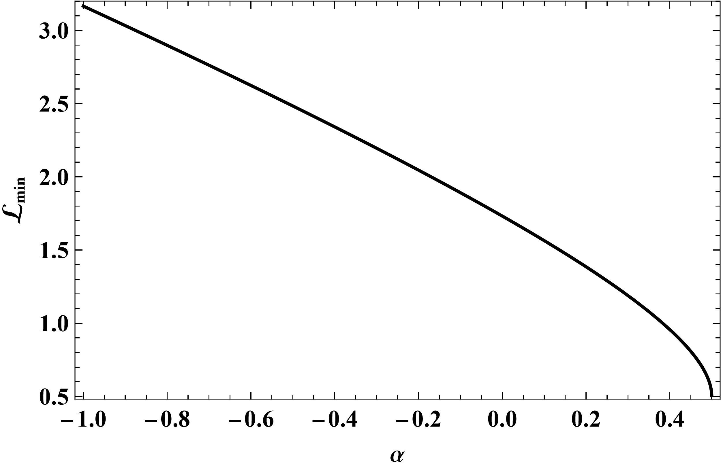
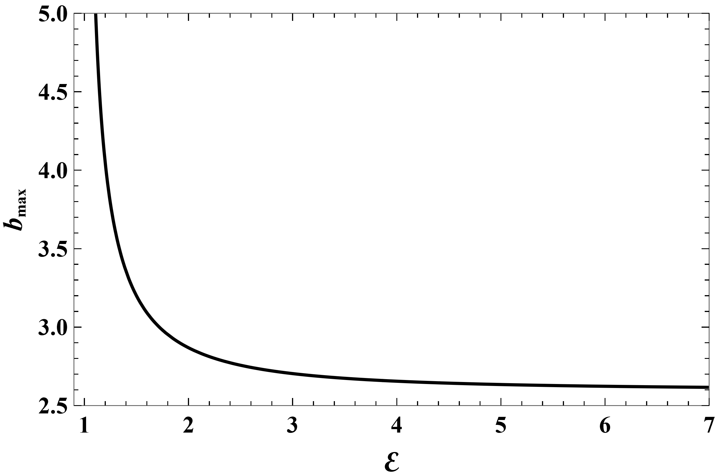
Figure 4 shows how depends on for several negative values of the coupling parameter . The effect of increasing is to increase the values of for all energies. This is expected because the Coulombs attraction makes it easier for a charges particle to get captured. In all cases, is a monotonic function of . In the ultra-relativistic limit, approaches , the limit in the neutral particle case, for any finite value of , provided that is not too large compared to .
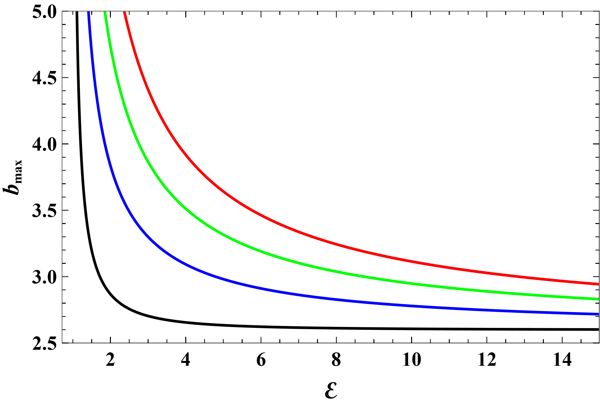
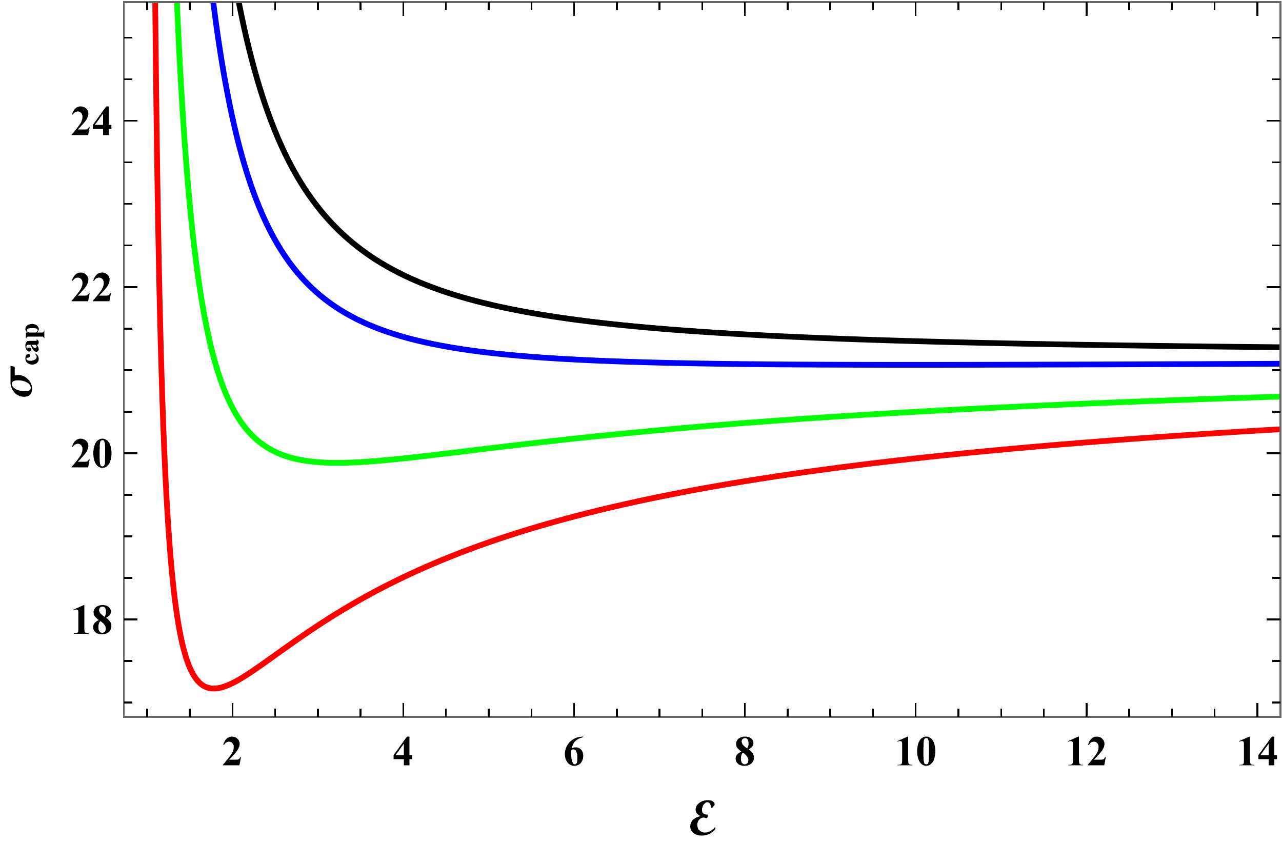
Figure 5 shows how depends on for several values of between and . In this range, there is competition between that gravitational ’attraction’ and the Coulomb repulsion. The curves have richer structure. They falls quickly as goes beyond and reach a minimum. After that, the curves rise and reach asymptotically.
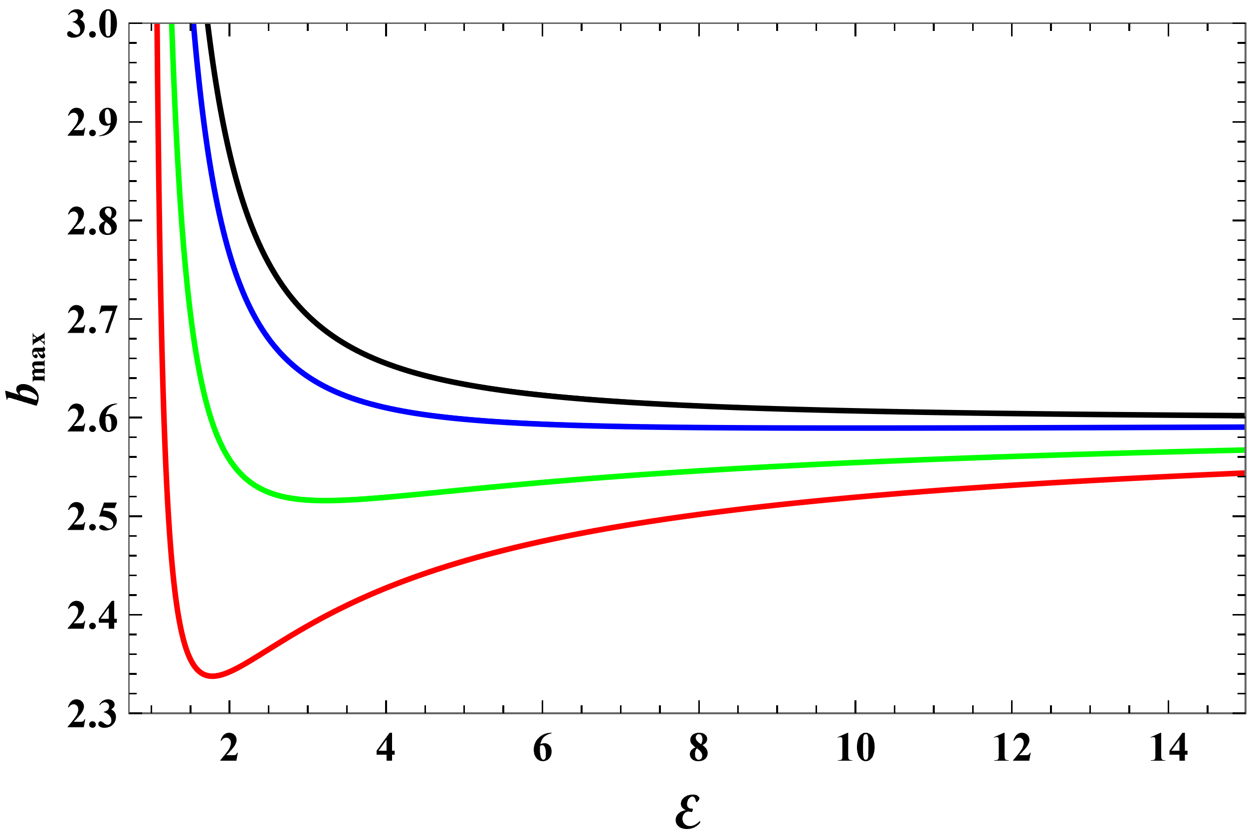
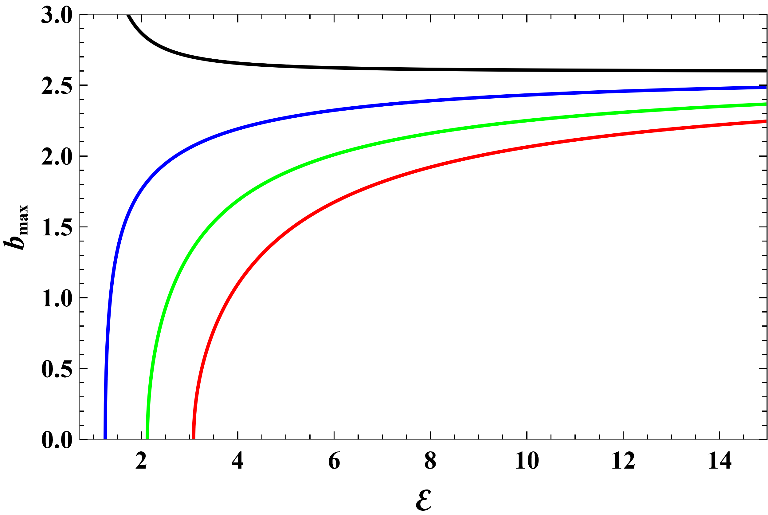
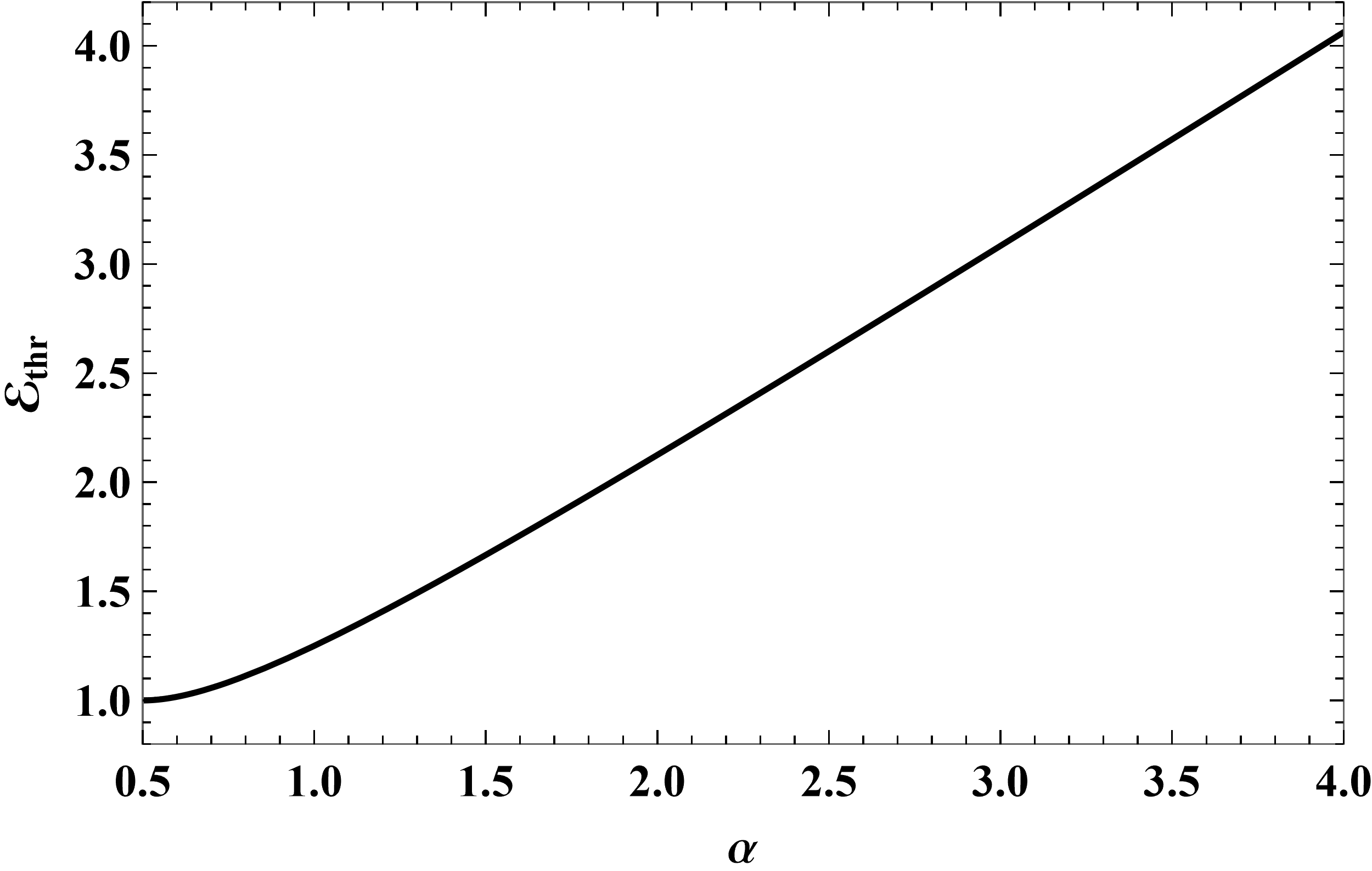
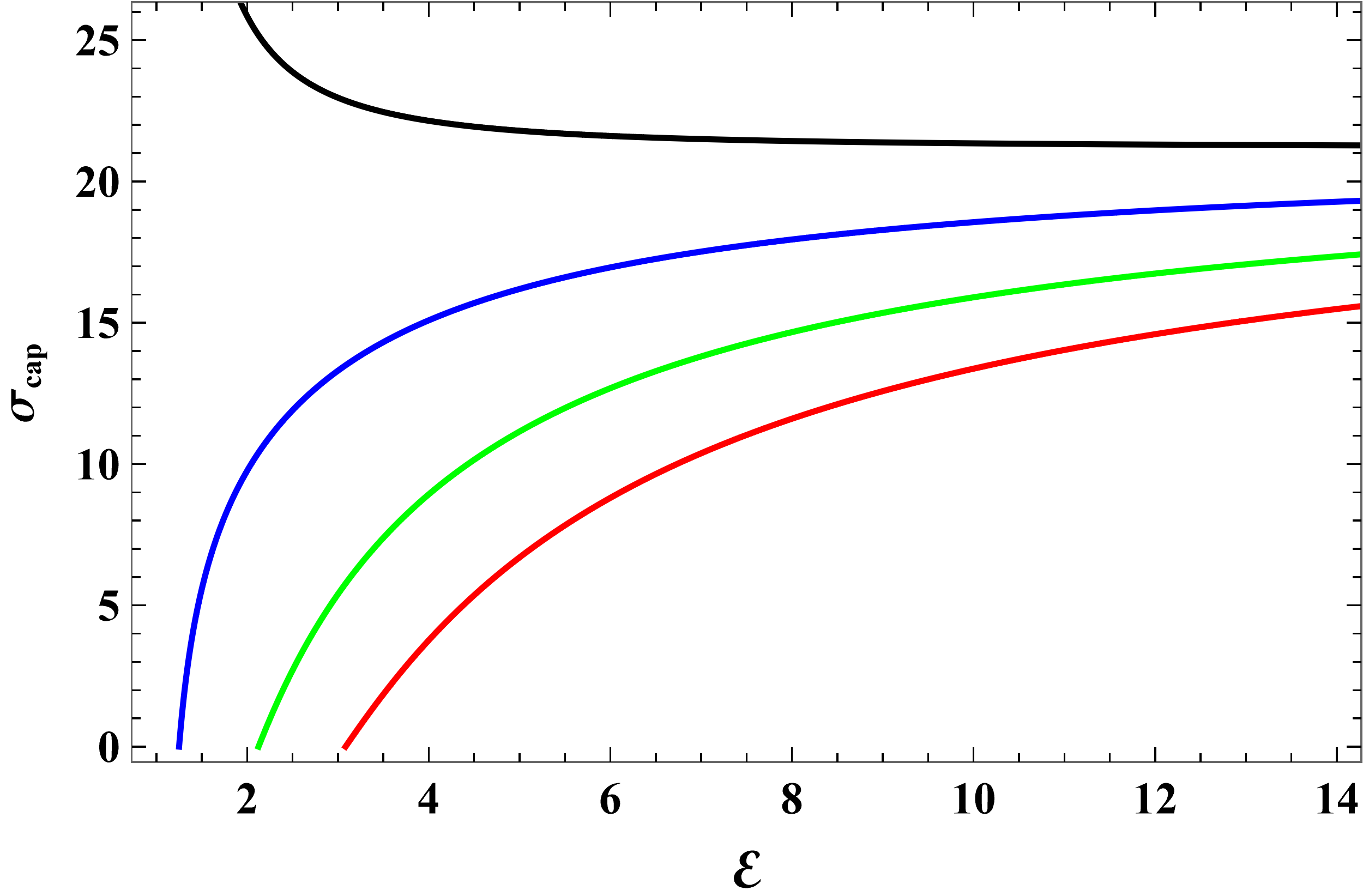
Figure 6 shows how depends on for several positive values of greater than . Generally, becomes smaller as increases. This is expected because the greater the Coulomb repulsion the more difficult it is for a charged particle to be captured. In fact, there is a threshold energy below which capture cannot occur. It is given by
| (35) |
This equation is valid for only. Fig. 7 shows how vary with .
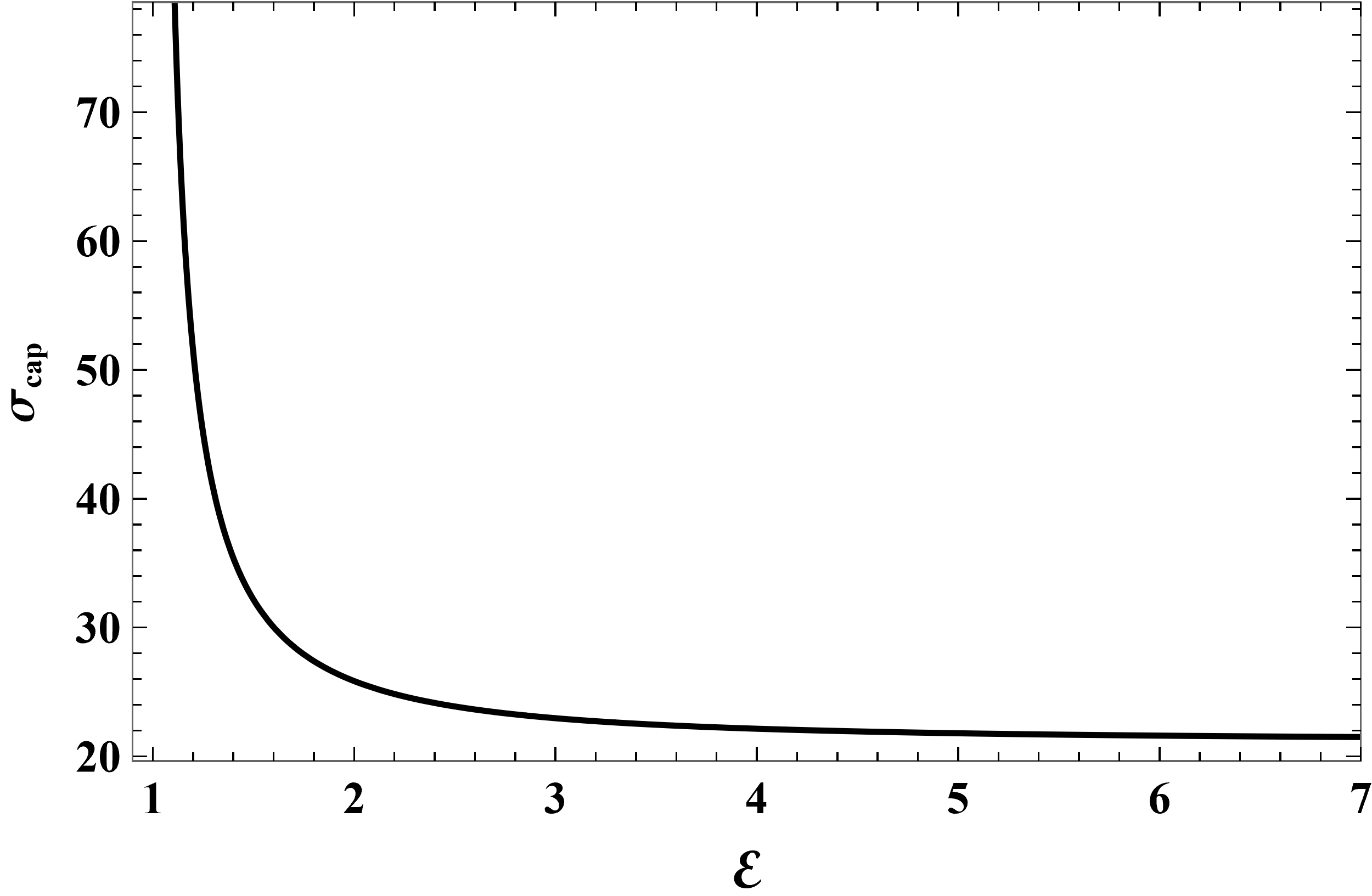
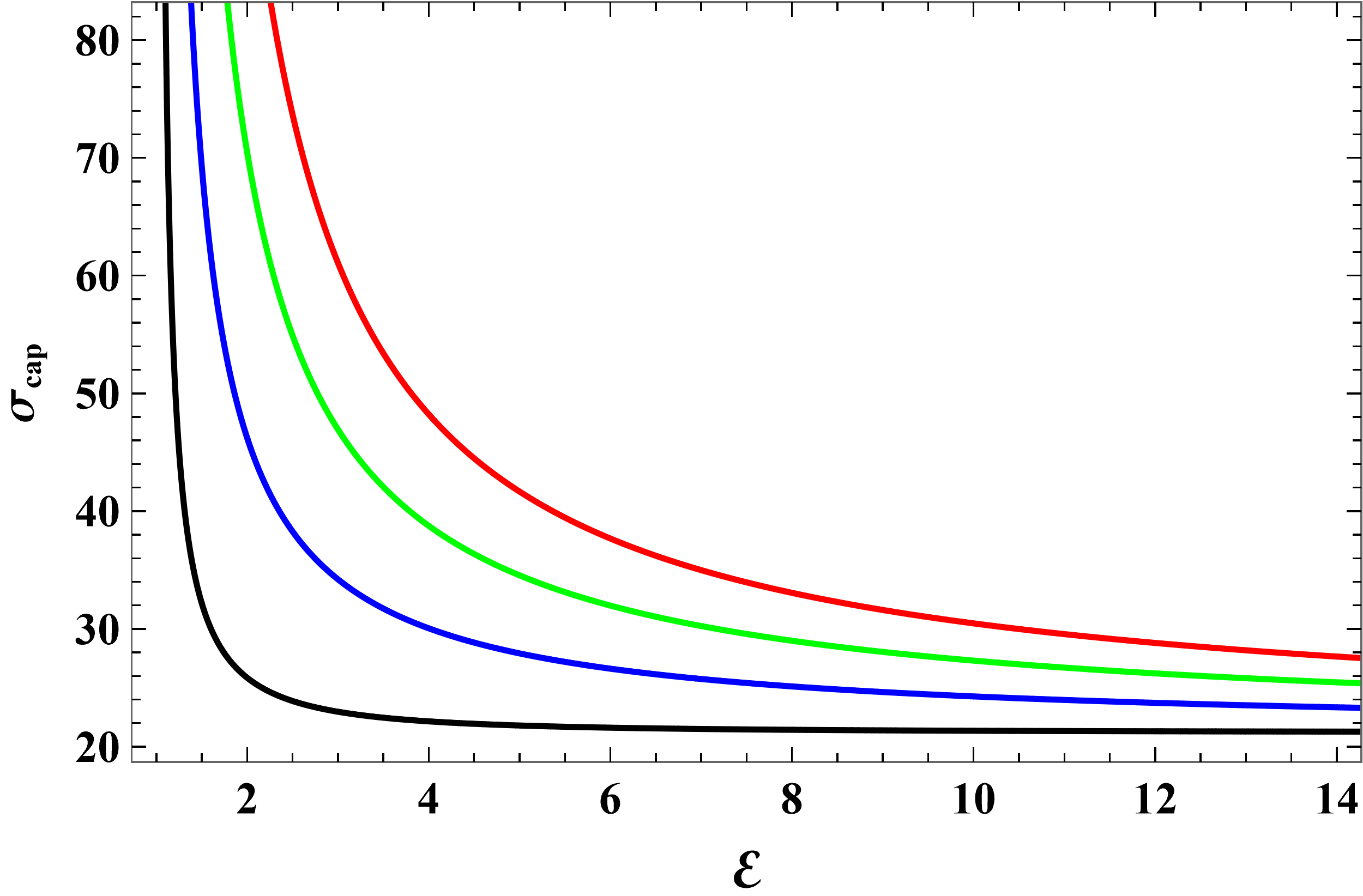
The capture cross-section corresponding to Figs. 4, 5 and 6 is shown in Figs. 8, 10 and 9, respectively. In all cases, vs. curves inherent the features of the vs. curves.
For ultra-relativistic particles, we can write as
| (36) |
The corresponding capture cross-section is then
| (37) |
These limiting results are in agreement with our numerical findings.
5 Conclusion
We have studied the capture cross-section of charged particles by a weakly charged Schwarzschild black hole. We have shown that a trace charge on the black hole can have prominent effects.
When the Coulomb force between a charged particle and the black hole is attractive, it enlarges the capture cross-section significantly. This is expected since the Coulomb attraction enhances the capture of charged particles. However, when the Coulomb force between a charged particle and the black hole is repulsive, it shrinks the capture cross-section significantly. When the electromagnetic coupling strength is below a critical value, capture is possible for all values of the particle’s energy. When the electromagnetic coupling strength is above the critical value, there is a minimum value of the particle’s energy below which capture is impossible. This is because the Coulomb repulsion surpasses the gravitational attraction unless the particle’s radial momentum is large enough.
Our results emphasizes the assertion that charged black holes will favorably accretes charges of the opposite sign. However, it is still possible for the black hole charge to grow if the plunging charged particles are energetic enough to the limit that the capture cross-section becomes independent of the sign of the charges. Moreover, the fact that the electromagnetic coupling constant is three orders of magnitudes greater for electrons than protons suggests that it is relatively easier for a black hole to accumulate positive charge than negative charge.
It will be an astrophysically interesting to study the energies of charged particles near an astrophysical black hole to understand better how the black hole’s charge evolves. The problem can be astrophyically more viable when other astrophysical black holes, such as rotating black holes, are studied (in progress).
References
- Ahmedov et al. (2021) Ahmedov B., Rahimov O., Toshmatov B., 2021, Universe, 7(8) , 307.
- Al Zahrani (2021) Al Zahrani A., 2021, Phys. Rev. D, 103.
- Al Zahrani (2022) Al Zahrani A., 2022, ApJ, 937.
- Anacleto, et al. (2023) Anacleto M., et al., 2023, arXiv:2307.09536v1 [gr-qc].
- Bugden (2020) Bugden M., 2020, Class. Quantum Gravity, 37, 015001.
- Carter (1973) Carter B., 1973, Black Hole Equilibrium States, Black Holes, eds. C. DeWitt and B. S. DeWitt (Gordon and Breach Science Publishers, Inc. New York, p. 57.
- Chandrasekhar (1983) Chandrasekhar S., 1983, The Mathematical Theory of Black Holes, Oxford University Press.
- Connell & Frolov (2008) Connell P., Frolov V., 2008, Phys. Rev. D, 78, 024032.
- Frolov & Zelnikov (2011) Frolov V., Zelnikov A., 2011, Introduction to black hole physics, Oxford university press.
- Ghosh & Afrin (2023) Ghosh S. and Afrin M., 2023, ApJ, 944, 174.
- Goldstein et al. (2001) Goldstein H., Poole C. and Safko J., 2001, Classical Mechanics, third eddition, Pearson.
- Gooding & Frolov (2008) Gooding C., Frolov A., 2008, Phys. Rev. D, 77, 104026.
- GRAVITY Collaboration (2023) GRAVITY Collaboration, 2023, A & A, 677, L10.
- Kocherlakota et al. (2021) Kocherlakota P. et al., 2021, (EHT Collaboration), Phys. Rev. D, 103, 104047.
- Misner et al. (1973) Misner C., Thorne K., Wheeler J., 1973, Gravitation, W. H. Freeman and Co., San Francisco.
- Singh & Ghosh (2018) Singh B. , Ghosh S., 2018, Annals of Physics 395, 127.
- Tsukamoto (2014) Tsukamoto N., et al., 2014, Phys. Rev. D, 90, 064043.
- Young (1976) Young P., 1976, Phys. Rev. D, 14, 3281.
- Zajaček et al. (2018) Zajaček M. et al., 2018, Monthly Notices of the Royal Astronomical Society, 480 4, 4408.
- Zajaček et al. (2019) Zajaček M. et al., 2019, J. Phys.: Conf. Ser., 1258, 012031.
- Zajaček & Tursunov (2019) Zajaček M., Tursunov A., arXiv:1904.04654.
- Zakharov (1994) Zakharov A., 1994, Class. Quantum Grav., 11, 1027.