Charmonium-like states with the exotic quantum number $J^{PC}=3^{-+}$

There have been many candidates for exotic hadrons observed in particle experiments, which can not be well explained in the traditional quark model pdg ; Liu:2019zoy ; Lebed:2016hpi ; Esposito:2016noz ; Guo:2017jvc ; Ali:2017jda ; Olsen:2017bmm ; Karliner:2017qhf ; Brambilla:2019esw ; Guo:2019twa . Many of them still have the “traditional” quantum numbers that the traditional $\bar{q}q$ mesons and $qqq$ baryons can form. This makes them not so easy to be clearly identified as exotic hadrons. However, there exist some “exotic” quantum numbers that the traditional hadrons can not form, such as the spin-parity quantum numbers $J^{PC}=0^{--}$, $0^{+-}$, $1^{-+}$, $2^{+-}$, $3^{-+}$, and $4^{+-}$, etc. These “exotic” quantum numbers are of particular interest, because the states with such quantum numbers can not be explained as traditional hadrons. Such states are definitely exotic hadrons, whose possible interpretations are tetraquark states Chen:2008qw ; Chen:2008ne ; Jiao:2009ra ; Huang:2016rro ; LEE:2020eif ; Du:2012pn ; Fu:2018ngx ; Dong:2022otb ; Xi:2023byo ; Dong:2022cuw ; Yang:2022rck ; Ji:2022blw ; Wang:2021lkg ; Wang:2023jaw , hybrid states Meyer:2015eta ; Chetyrkin:2000tj ; Zhang:2013rya ; Huang:2014hya ; Huang:2016upt ; Ho:2018cat ; Wang:2023whb ; Su:2023jxb ; Tan:2024grd ; Chen:2022isv ; Dudek:2013yja ; Li:2021fwk ; Tang:2021zti ; Qiu:2022ktc ; Wan:2022xkx ; Wang:2022sib ; Frere:2024wsf ; Barsbay:2024vjt , and glueballs Qiao:2014vva ; Tang:2015twt ; Pimikov:2017bkk , etc. Note that these exotic structures may mix together, making it challenging to arrive at a clear differentiation.

Among the above exotic quantum numbers, the hybrid states of $J^{PC}=1^{-+}$ have been extensively studied in literature, since they are predicted to be the lightest hybrid states Meyer:2015eta , and there have been some experimental evidences on their existence E852:1997gvf ; CrystalBarrel:1999reg ; E862:2006cfp . The light tetraquark states of $J^{PC}=1^{-+}$ have also been studied in Refs. Chen:2008qw ; Chen:2008ne using the method of QCD sum rules, and their masses and possible decay channels were predicted there for both the isospin-0 and isospin-1 states. Later the same QCD sum rule method was applied to extensively study the light tetraquark states of $J^{PC}=0^{--}/0^{+-}/2^{+-}/4^{+-}$ in Refs. Jiao:2009ra ; Huang:2016rro ; LEE:2020eif ; Du:2012pn ; Fu:2018ngx ; Dong:2022otb ; Xi:2023byo .

In this paper we shall study the exotic quantum number $J^{PC}=3^{-+}$ using the method of QCD sum rules. The light $qs\bar{q}\bar{s}$ tetraquark states ($q=up/down$ and $s=strange$) with such a quantum number have been systematically investigated in Ref. Su:2020reg , and in this paper we shall further study their corresponding charmonium-like $qc\bar{q}\bar{c}$ tetraquark states. These states are potential exotic hadrons to be observed in the future BESIII, Belle-II, and LHCb experiments. There are just a few theoretical studies on this subject. In Ref. Zhu:2013sca the authors used the one-boson-exchange model to study the $D^{*}\bar{D}_{2}^{*}$ molecular state of $J^{PC}=3^{-+}$, and their results suggest its possible existence. In Ref. Dong:2021juy the authors further investigated this state by solving the Bethe-Salpeter equation. Additionally, there was a Lattice QCD study on the $J^{PC}=3^{-+}$ glueball Shen:1984mxq .

This paper is organized as follows. In Sec. II, we systematically construct the $qc\bar{q}\bar{c}$ tetraquark currents with the exotic quantum number $J^{PC}=3^{-+}$. Then we apply the QCD sum rule method to study them in Sec. III, and perform numerical analyses in Sec. IV. The obtained results are summarized and discussed in Sec. V.

In this section we construct the hidden-charm tetraquark currents with the exotic quantum number $J^{PC}=3^{-+}$. We have systematically constructed the hidden-strange tetraquark currents with such a quantum number in Ref. Su:2020reg , and in this paper we just need to replace the $strange$ quarks by the $charm$ quarks. Note that the exotic quantum number $J^{PC}=3^{-+}$ can not be simply reached by using one quark field and one antiquark field, while it can not be reached by using two quark fields and two antiquark fields neither. Actually, we need two quark fields and two antiquark fields together with at least one derivative to reach such a quantum number.

As the first step, we work within the diquark-antidiquark configuration, where the derivative can be either inside the diquark/antidiquark field or between them ($c=charm$ and $q=up/down$):

Here $a\cdots d$ are color indices, and the sum over repeated indices is taken; $\Gamma_{1\cdots 4}$ are Dirac matrices; $\big{[}X{\overset{\leftrightarrow}{D}}_{\alpha}Y\big{]}=X[D_{\alpha}Y]-[D_{\alpha}X]Y$ with the covariant derivative $D_{\alpha}=\partial_{\alpha}+ig_{s}A_{\alpha}$. We find that only the former two can be combined to reach the exotic quantum number $J^{PC}=3^{-+}$.

There are altogether six independent diquark-antidiquark currents of $J^{PC}=3^{-+}$:

where $\mathcal{S}$ denotes symmetrization and subtracting the trace terms in the set $\{\alpha_{1}\alpha_{2}\alpha_{3}\}$, so that the spin-3 components can be well separated. Three of them $\eta^{1,3,5}_{\alpha_{1}\alpha_{2}\alpha_{3}}$ have the antisymmetric color structure $(qc)_{\mathbf{\bar{3}}_{C}}(\bar{q}\bar{c})_{\mathbf{3}_{C}}$, and the other three $\eta^{2,4,6}_{\alpha_{1}\alpha_{2}\alpha_{3}}$ have the symmetric color structure $(qc)_{\mathbf{6}_{C}}(\bar{q}\bar{c})_{\mathbf{\bar{6}}_{C}}$.

Besides the diquark-antidiquark configuration, we also investigate the meson-meson configuration. There are six independent meson-meson currents of $J^{PC}=3^{-+}$:

We can apply the Fierz rearrangement to relate the above diquark-antidiquark and meson-meson currents:

Hence, these two configurations are equivalent, and we shall apply this Fierz identity to study the decay properties at the end of this paper. However, this equivalence is just between the local diquark-antidiquark and meson-meson currents, while the tightly-bound diquark-antidiquark tetraquark states and the weakly-bound meson-meson molecular states are totally different. To clearly describe them, we need to investigate the non-local currents, which can not be done within the QCD sum rule framework yet.

In this section we apply the QCD sum rule method to study the six diquark-antidiquark currents $\eta^{i}_{\alpha_{1}\alpha_{2}\alpha_{3}}$ ($i=1\cdots 6$), and calculate their two-point correlation functions

at both the hadron and quark-gluon levels. Here $\tilde{g}_{\mu\nu}=g_{\mu\nu}-q_{\mu}q_{\nu}/q^{2}$, and $\mathcal{S}^{\prime}$ denotes symmetrization and subtracting trace terms in the two sets $\{\alpha_{1}\alpha_{2}\alpha_{3}\}$ and $\{\beta_{1}\beta_{2}\beta_{3}\}$.

Take the first current $\eta^{1}_{\alpha_{1}\alpha_{2}\alpha_{3}}$ as an example. We assume that it couples to the possibly-existing exotic state $X_{1}$ through

with $f_{1}$ the decay constant. The symmetric and traceless polarization tensor $\epsilon_{\alpha_{1}\alpha_{2}\alpha_{3}}$ satisfies

At the hadron level we apply the dispersion relation to write Eq. (III) as:

with $\rho^{\rm phen}_{11}(s)$ the phenomenological spectral density. We parameterize it using one pole dominance for the state $X_{1}$ and a continuum contribution

At the quark-gluon level we insert the current $\eta^{1}_{\alpha_{1}\alpha_{2}\alpha_{3}}$ into Eq. (III), and calculate it using the method of operator product expansion (OPE), from which we extract the OPE spectral density $\rho_{11}(s)\equiv\rho_{11}^{\rm OPE}(s)$. Then we perform the Borel transformation at both the hadron and quark-gluon levels. After approximating the continuum using the OPE spectral density above the threshold value $s_{0}$, we obtain the QCD sum rule equation

We can use it to further calculate $M_{1}$ through

The OPE spectral density $\rho_{11}(s)$ extracted from the current $\eta^{1}_{\alpha_{1}\alpha_{2}\alpha_{3}}$ is

where

In the above expressions, $\mathcal{F}(s)=\left[(\alpha+\beta)m_{c}^{2}-\alpha\beta s\right]$, $\mathcal{H}(s)=\left[m_{c}^{2}-\alpha(1-\alpha)s\right]$, $\alpha_{\min}=\frac{1-\sqrt{1-4m_{c}^{2}/s}}{2}$, $\alpha_{\max}=\frac{1+\sqrt{1-4m_{c}^{2}/s}}{2}$, $\beta_{\min}=\frac{\alpha m_{c}^{2}}{\alpha s-m_{c}^{2}}$, and $\beta_{\max}=1-\alpha$. We have calculated the QCD spectral density $\rho_{11}(s)$ at the leading order of $\alpha_{s}$ and up to the dimension ten ($D=10$). In the calculations we have considered the perturbative term, the charm quark mass, the quark condensate $\langle\bar{q}q\rangle$, the gluon condensate $\langle g_{s}^{2}GG\rangle$, the quark-gluon mixed condensate $\langle g_{s}\bar{q}\sigma Gq\rangle$, and their combinations. We have ignored the chirally suppressed terms with light quark masses, and we have adopted the factorization assumption of vacuum saturation for higher dimensional condensates. We find that the $D=3$ term $\langle\bar{q}q\rangle$ and the $D=5$ term $\langle g_{s}\bar{q}\sigma Gq\rangle$ are both multiplied by the charm quark mass, so they are important power corrections to the correlation functions. The QCD sum rule results extracted from the other five currents $\eta^{2\cdots 6}_{\alpha_{1}\alpha_{2}\alpha_{3}}$ are given in Appendix A. Based on these results, we shall perform numerical analyses in the next section.

In this section we use the spectral densities given in Eq. (43) and Eqs.(59-63) to perform numerical analyses. We shall use the following values for various QCD sum rule parameters Yang:1993bp ; Narison:2002hk ; Gimenez:2005nt ; Jamin:2002ev ; Ioffe:2002be ; Ovchinnikov:1988gk ; Ellis:1996xc ; Narison:2011xe ; Narison:2018dcr ; pdg :

The gluon condensate $\langle g_{s}^{2}GG\rangle$ is still not well known, and the above value for this condensate is taken from Ref. Narison:2018dcr , which was updated in 2018. We note that this condensate does not contribute much to the spectral densities. Different with some other QCD sum rule calculations Su:2023jxb ; Tan:2024grd , there is a minus sign in the definition of the mixed condensate $\langle g_{s}\bar{q}\sigma Gq\rangle$, which is just because the definition of coupling constant $g_{s}$ is different Yang:1993bp ; Hwang:1994vp , i.e., $D_{\alpha}=\partial_{\alpha}+ig_{s}A_{\alpha}$ is used the present study, while $D_{\alpha}=\partial_{\alpha}-ig_{s}A_{\alpha}$ is used in Refs. Su:2023jxb ; Tan:2024grd .

We take the spectral density $\rho_{11}(s)$ extracted from the current $\eta^{1}_{\alpha_{1}\alpha_{2}\alpha_{3}}$ as an example. As shown in Eq. (III), the mass $M_{X}$ and the decay constant $f_{X}$ both depend on two free parameters: the threshold value $s_{0}$ and the Borel mass $M_{B}$. We investigate three aspects to find their proper working regions: a) the convergence of OPE, b) the one-pole-dominance assumption, and c) the mass dependence and the decay constant dependence on these two parameters.

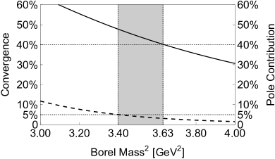
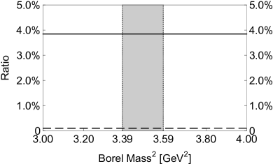
Firstly, we investigate the convergence of OPE and require the $D=10$ terms to be less than 5%:

As shown in Fig. 1, we determine the lower bound of the Borel mass to be $M_{B}^{2}\geq 3.40$ GeV².

Secondly, we investigate the one-pole-dominance assumption and require the pole contribution (PC) to be larger than 40%:

As shown in Fig. 1, we determine the upper bound of the Borel mass to be $M_{B}^{2}\leq 3.63$ GeV² when setting $s_{0}=30.0$ GeV². Altogether we determine the Borel window to be $3.40$ GeV${}^{2}\leq M_{B}^{2}\leq 3.63$ GeV² when setting $s_{0}=30.0$ GeV². After changing $s_{0}$ and redoing the same procedures, we find that there are non-vanishing Borel windows as long as $s_{0}\geq s_{0}^{\rm min}=28.4$ GeV².

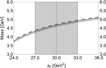
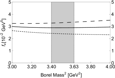
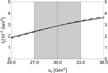
Thirdly, we investigate the mass dependence and the decay constant dependence on $s_{0}$ and $M_{B}$. We respectively show the mass $M_{1}$ in Fig. 2 and the decay constant $f_{1}$ in Fig. 3 as functions of these two parameters. Their dependence on $M_{B}$ is weak inside the Borel window $3.40$ GeV${}^{2}\leq M_{B}^{2}\leq 3.63$ GeV², and their dependence on $s_{0}$ is moderate and acceptable around $s_{0}\sim 30.0$ GeV². Accordingly, we choose our working regions to be $27.0$ GeV${}^{2}\leq s_{0}\leq 33.0$ GeV² and $3.40$ GeV${}^{2}\leq M_{B}^{2}\leq 3.63$ GeV², where the mass $M_{1}$ is evaluated to be

Its central value corresponds to $s_{0}=30.0$ GeV² and $M_{B}^{2}=3.52$ GeV². Its uncertainty is due to $s_{0}$, $M_{B}$, and various QCD sum rule parameters listed in Eqs. (44).

We apply the same procedures to study the other five currents $\eta^{2\cdots 6}_{\alpha_{1}\alpha_{2}\alpha_{3}}$, and summarize their results in Table 1. Especially, the mass $M_{2}$ extracted from the current $\eta^{2}_{\alpha_{1}\alpha_{2}\alpha_{3}}$ is calculated to be

which is slightly smaller than the mass $M_{1}$ extracted from the current $\eta^{1}_{\alpha_{1}\alpha_{2}\alpha_{3}}$, while the masses extracted from the other four currents $\eta^{3\cdots 6}_{\alpha_{1}\alpha_{2}\alpha_{3}}$ are all significantly larger.

It is interesting to investigate the mixing of $\eta^{1}_{\alpha_{1}\alpha_{2}\alpha_{3}}$ and $\eta^{2}_{\alpha_{1}\alpha_{2}\alpha_{3}}$ by calculating their off-diagonal correlation function, i.e., the “12” component of Eq. (III):

To see how large it is, we choose $s_{0}=29.0$ GeV² and $M_{B}^{2}=3.40$ GeV² to obtain