Chemical Cartography with APOGEE: Mapping Disk Populations with a Two-Process Model and Residual Abundances
Abstract
We apply a novel statistical analysis to measurements of 16 elemental abundances in 34,410 Milky Way disk stars from the final data release (DR17) of APOGEE-2. Building on recent work, we fit median abundance ratio trends [X/Mg] vs. [Mg/H] with a 2-process model, which decomposes abundance patterns into a “prompt” component tracing core collapse supernovae and a “delayed” component tracing Type Ia supernovae. For each sample star, we fit the amplitudes of these two components, then compute the residuals from this two-parameter fit. The rms residuals range from dex for the most precisely measured APOGEE abundances to dex for Na, V, and Ce. The correlations of residuals reveal a complex underlying structure, including a correlated element group comprised of Ca, Na, Al, K, Cr, and Ce and a separate group comprised of Ni, V, Mn, and Co. Selecting stars poorly fit by the 2-process model reveals a rich variety of physical outliers and sometimes subtle measurement errors. Residual abundances allow comparison of populations controlled for differences in metallicity and [/Fe]. Relative to the main disk (), we find nearly identical abundance patterns in the outer disk (), 0.05-0.2 dex depressions of multiple elements in LMC and Gaia Sausage/Enceladus stars, and wild deviations (0.4-1 dex) of multiple elements in Cen. Residual abundance analysis opens new opportunities for discovering chemically distinctive stars and stellar populations, for empirically constraining nucleosynthetic yields, and for testing chemical evolution models that include stochasticity in the production and redistribution of elements.
.
1 Introduction
Over the past decade, large and systematic spectroscopic surveys have mapped elemental abundance patterns of hundreds of thousands of stars across much of the Galactic disk, bulge, and halo, including RAVE, SEGUE, LAMOST, Gaia-ESO, APOGEE, GALAH, and H3 (Steinmetz et al., 2006; Yanny et al., 2009; Luo et al., 2015; Gilmore et al., 2012; De Silva et al., 2015; Majewski et al., 2017; Conroy et al., 2019). The APOGEE survey of SDSS-III (Eisenstein et al., 2011) and SDSS-IV (Blanton et al., 2017) is especially well suited to mapping the inner disk and bulge because it observes at near-IR wavelengths where dust obscuration is dramatically reduced, because it targets luminous evolved stars that can be observed at large distances, and because its high spectral resolution allows separate determinations of 15 or more elemental abundances per target star.111SDSS = Sloan Digital Sky Survey. APOGEE = Apache Point Observatory Galactic Evolution Experiment. We use APOGEE to refer to both the SDSS-III program and its SDSS-IV extension (a.k.a. APOGEE-2). In SDSS-V (Kollmeier et al., 2017) the Milky Way Mapper program is using the APOGEE spectrographs to observe a sample ten times larger than that of SDSS-III + IV. These surveys share two primary goals: to understand the astrophysical processes that govern the synthesis of the elements, and to trace the chemical evolution of the Milky Way, which is itself shaped by many processes including gas accretion, star formation, outflows, and radial migration of stars. This paper introduces a novel approach to characterizing and mapping abundance patterns in APOGEE, one that opens new avenues to addressing both of these goals.
Our study builds on a series of investigations that have used APOGEE data to characterize the multi-element abundance distributions of the Galactic disk and bulge (Anders et al., 2014; Hayden et al., 2014, 2015; Nidever et al., 2014; Ness et al., 2016; Ting et al., 2016; Mackereth et al., 2017; Schiavon et al., 2017; Bovy et al., 2019; Fernández-Trincado et al., 2019a, 2020b; Weinberg et al., 2019; Zasowski et al., 2019; Griffith et al., 2021a; Ting & Weinberg, 2021; Vincenzo et al., 2021a). Its most direct predecessors are the papers of Hayden et al. (2015, hereafter H15), who mapped the distribution of stars in as a function of Galactocentric radius and midplane distance , and Weinberg et al. (2019, hereafter W19), who examined the median trends of other abundance ratios as a function of and . Because elements such as O, Mg, and Si are produced mainly by core collapse supernovae (CCSN), while Fe is produced by both CCSN and Type Ia supernovae (SNIa), the ratio is a diagnostic of the relative contribution of these two sources to a star’s chemical enrichment. Many studies have shown that stars in the solar neighborhood have a bimodal distribution of , with “thin disk” stars having roughly solar abundance ratios and “thick disk” stars (which have larger vertical velocities and consequently larger excursions from the disk midplane) having elevated (e.g., Fuhrmann 1998; Bensby et al. 2003; Adibekyan et al. 2012; Vincenzo et al. 2021a). H15 showed that the locus of the “high-” sequence in the plane is nearly constant throughout the disk (see also Nidever et al. 2014) but the relative number of high- and low- stars and the distribution of those stars in changes systematically with and . W19 advocated the use of Mg rather than Fe as a reference element because it traces a single enrichment source (CCSN), and they showed that the median trends of for nearly all of the elements measured by APOGEE are universal throughout the disk, provided that one separates the high- and low- populations. Griffith et al. (2021a) showed that this universality of abundance ratio trends extends to the bulge.
Since the star formation and enrichment histories do change across the Galaxy, W19 argued that the universal median sequences must be determined mainly by IMF-averaged nucleosynthetic yields.222IMF = Initial Mass Function They interpreted these sequences in terms of a “2-process model,” which describes APOGEE abundances as the sum of a core collapse process representing the IMF-averaged yields of CCSN and a Type Ia process reflecting the IMF-averaged yields of SNIa. The elemental abundances of a given star can be summarized by the two parameters and that scale the amplitudes of these processes. The success of the 2-process model means that all of a disk or bulge star’s APOGEE abundances can be predicted to surprisingly high accuracy from its Mg and Fe abundances alone. They can be predicted to similar accuracy from the combination of and age (Ness et al., 2019). Nonetheless, the residual abundances of other elements at fixed and contain rich information, as demonstrated empirically by Ting & Weinberg (2021, hereafter TW21), who show that one must condition on at least seven APOGEE elements (e.g., Fe, Mg, O, Si, Ni, Ca, Al) before the correlations among the remaining abundances are reduced to a level consistent with observational uncertainties. In this paper, therefore, we turn our attention from median trends to the star-by-star abundance patterns described by 2-process model parameters and the residuals from this description. As argued by TW21, the correlations of residual abundances encode crucial information about nucleosynthetic processes and stochastic effects in chemical evolution.
Although “high-” stars have elevated compared to the Sun, this difference really arises because they have a lower contribution of SNIa to Fe rather than enhanced production of elements by CCSN (Tinsley, 1980; Matteucci & Greggio, 1986; McWilliam, 1997). Adopting this physical interpretation, we will refer to high- and low- stars in this paper as the “low-Ia” and “high-Ia” populations, respectively, following terminology introduced by Griffith et al. (2019).
In §2 we describe the 2-process model, which is similar to that of W19 and Griffith et al. (2019) but with adjustments that make the model more flexible and easier to generalize. In §3 we describe our selection of APOGEE stars from SDSS Data Release 17 (DR17): red giants in a restricted range of , , and intended to minimize statistical and differential systematic errors while sampling the disk in the range and . Section 4 presents median abundance trends from this sample and uses them to infer the CCSN and SNIa 2-process vectors, i.e., the abundance of each of the APOGEE elements associated with these two processes at a given metallicity. In §5, the heart of the paper, we fit each sample star’s abundances with the 2-process model and examine the distributions and correlations of the abundance residuals. As in TW21, we find a rich correlation structure among these residuals, and we further examine the correlation of these residuals with stellar age and kinematics. In §6 we investigate stars whose abundance patterns deviate unusually far from the 2-process model fits, a group that includes both genuine physical outliers and stars with measurement errors that exceed the reported uncertainties. In §7 we examine the residual abundances of a few special populations, such as likely halo stars that reside within the geometrical boundaries of the disk and members of the rich cluster Cen, which is thought to be the stripped core of an accreted dwarf spheroidal galaxy. Section 8 discusses ways to go beyond the 2-process model, first with a conceptual -process formulation, then with an empirical approach that fits two additional components to the APOGEE abundance residuals. We review our conclusions and outline prospects for future studies in §9.
This is a long paper covering many interconnected topics. Readers who want to start with a bird’s-eye view can read the introduction to the 2-process model at the start of §2, look through figures with particular attention to the median trends (Figure 4-7), distributions and covariance of residual abundances (Figures 12 and 15), examples of high- stars (Figure 20), and residual patterns of selected populations (Figure 22), then read the conclusions and loop back to earlier sections as needed. For readers interested in overall abundance trends and their interpretation, §4 is the most relevant. For readers interested in unusual stars and stellar populations, §6 and §7 are the most relevant. Readers interested in the dimensionality of the stellar distribution in abundance space and its connection to the physics of nucleosynthesis and chemical evolution should pay particular attention to §5 and §8. The challenge of determining accurate, precise, robust abundances for many elements in large stellar samples is a running theme throughout the paper.
2 The 2-process model
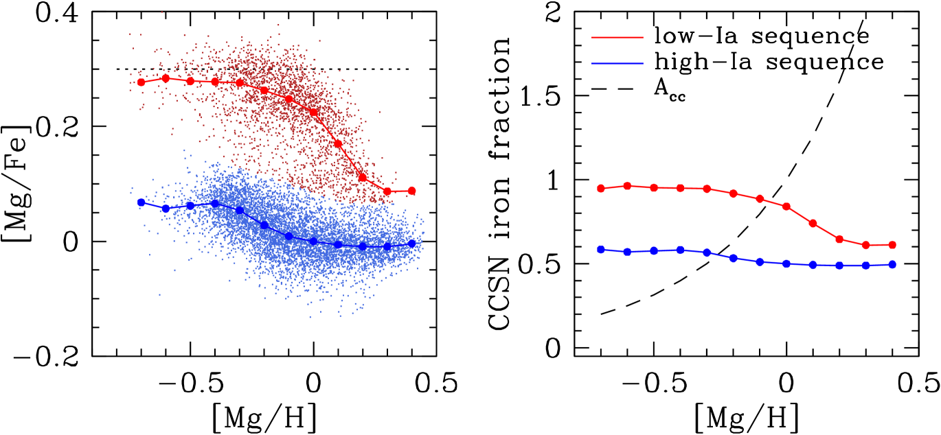
We begin with a conceptual introduction to the 2-process model. The left panel of Figure 1 shows the distribution of our APOGEE sample (described in §3) in the familiar plane of vs. , with the low-Ia and high-Ia populations as red and blue points, respectively. Like W19, we adopt as our reference abundance on the -axis because Mg is well measured in APOGEE and, unlike Fe, it is thought to come from a single nucleosynthetic source (CCSN).333We choose Mg in preference to O because the observed trends for O are significantly different between optical and near-IR surveys. We choose Mg in preference to Si or Ca because these have non-negligible SNIa contributions. In the conventional interpretation of this diagram, which we adopt in this paper, the “plateau” in the abundances of metal-poor low-Ia stars at represents the Mg/Fe ratio of CCSN yields, and stars that lie below this plateau do so primarily because they have additional Fe from SNIa. While the relative number of low-Ia and high-Ia stars depends strongly on Galactic location, the median tracks of these populations, shown by red and blue lines in Figure 1, are nearly universal throughout the disk (Nidever et al. 2014; H15; W19). The median tracks for other APOGEE elements are also universal throughout the disk (W19) and bulge (Griffith et al., 2021a), provided that one separates the low-Ia and high-Ia populations. This universality motivates the hypothesis that these tracks are governed by stellar yields and that differences between the two [X/Mg] tracks reflect the contribution of SNIa enrichment to element X.
In the 2-process model, the position of a star in the -dimensional space of its measured abundances is approximated as the weighted sum of two “vectors” that represent the contributions from CCSN and SNIa:
| (1) |
The 2-process vectors and are taken to be universal for the stellar sample under study, though they may depend on metallicity. The amplitudes and vary from star to star, and they are normalized such that for solar abundances. For notational compactness we define metallicity by
| (2) |
i.e., the Mg abundance in solar units. As discussed in §§2.1-2.3 below, we infer and from median abundance ratios of low-Ia and high-Ia stars, then determine and for all stars in the observational sample by a fit to a subset of their measured abundances.
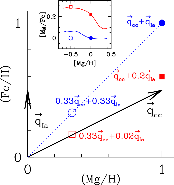
Figure 2 illustrates the simple case of dimensions, with points marking the location of four representative stars in (Fe/H) vs. (Mg/H), expressed in solar units. The 2-process (Mg,Fe) vectors are and , reflecting our model assumptions that Mg is produced entirely by CCSN and that solar Fe comes equally from CCSN and SNIa. The filled blue circle has solar abundances, with and . The open blue circle has , so its (Mg/H) and (Fe/H) abundances are 1/3 solar but its (Mg/Fe) ratio is solar. Filled and open red squares represent low-Ia stars with and , respectively. These stars have , so they have (Mg/Fe) ratios above solar (“-enhanced” or “iron poor”). With , the two parameters and suffice to fit each star’s abundances perfectly, but they recast the information from the space of individual elements to the space of the processes that produce those elements.
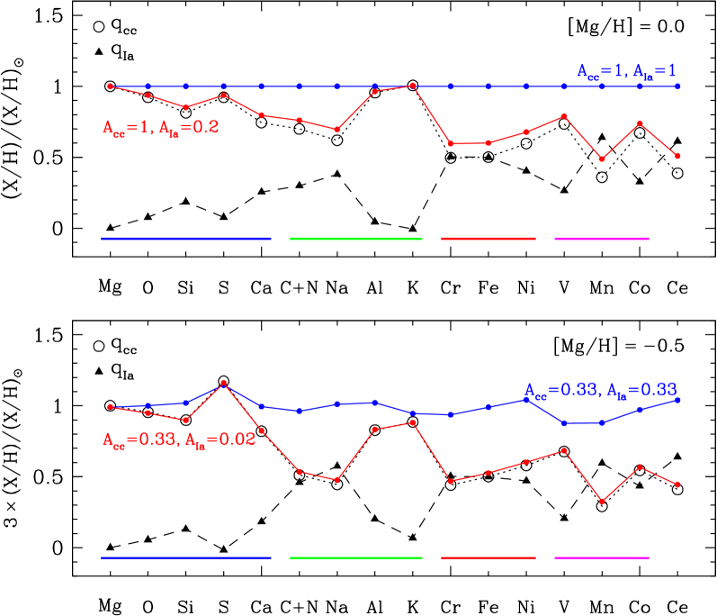
Using the same four combinations of as Figure 2, Figure 3 illustrates the 2-process model for the full set of 16 abundances that we consider in this paper, one of which is the element combination C+N (eq. 27 in §3). In the upper panel, open circles and filled triangles show the components of and that we derive from the APOGEE median abundance trends in §4 below, at metallicity . For -elements (on the left), values are much larger than values, while for iron-peak elements (on the right) they are roughly equal. For , the predicted abundances are exactly solar by construction (blue points). For and , the predicted abundances (red points) are only slightly above (black open circles), with sub-solar (X/H) values for all elements that have a substantial SNIa contribution in the Sun.
The lower panel shows our inferred 2-process vectors for (). These vectors are similar to those found at , but they are not identical because some elements have metallicity dependent yields. As a result, the predicted abundances for have element ratios that are approximately but not exactly solar (blue points). For a star on the low-Ia (high-) plateau, the predicted abundances (red points) are just slightly above . The predicted abundances (blue and red points) are multiplied by a factor of three so that the patterns can be visually compared to those of the stars shown in the upper panel.
With 16 abundances, any given star will not be perfectly reproduced by a 2-parameter fit, in part because of measurement errors, but also because the 2-process model is not a complete physical description of stellar abundances. For example, the model does not allow for stochastic variations around IMF-averaged yields or for varying contributions from other sources such as AGB enrichment. The 2-process vectors themselves are useful tests of supernova nucleosynthesis predictions (e.g., Griffith et al. 2019, 2021b), and the distributions of and their correlations with stellar age and kinematics are useful diagnostics of Galactic chemical evolution. However, our primary focus in this paper will be the star-by-star departures from the 2-process predictions, and what these departures can tell us about the astrophysical sources of the APOGEE elements, about distinct stellar populations within the geometric boundaries of the Milky Way disk, and about rare stars with distinctive abundance patterns. Disk stars span a range of dex in [Fe/H] and typically 0.3 dex or more in [X/Fe]. With two free parameters, the 2-process model fits the measured APOGEE abundances of most disk stars to within dex, and for the best measured elements to within dex, so focusing on these residual abundances allows us to discern subtle patterns that might be lost within the much larger dynamic range of a conventional [X/Fe]-[Fe/H] analysis.
We now proceed to a more formal definition of the 2-process model and its assumptions, and our methods for inferring the 2-process vectors and fitting and values. While our approach is similar to that of W19, here we define the model in a way that is more general and allows natural extension to include other processes as discussed in §8.
2.1 Model assumptions and basic equations
We can express equation (1) in the alternative form
| (3) |
with
| (4) |
While it may seem gratuitous to introduce both and , many of our equations can be written more compactly in terms of , and these two forms of the process vectors respond differently to changes in the adopted solar abundance values. For example, if stellar abundances are inferred by purely ab initio model-fitting then the vectors are directly determined while the vectors depend on adopted solar abundances. Conversely, if zero-point offsets are used to calibrate the abundance scale to reproduce solar values, then the vectors are directly determined and the conversion to vectors depends on the adopted solar abundances. At a given , is a set of discrete values, one for each element X being modeled, and likewise for . For brevity, we will frequently drop the explicit -dependence of and in our equations if it is not needed for clarity, but it is only for Mg and Fe that we assume that these processes are actually independent of metallicity.
We define in the Sun. Therefore, if we ignore the possible contribution of other processes,
| (5) |
for all X. In a star with metallicity and amplitudes and , the fraction of element that arises from CCSN is
| (6) | |||||
| (7) |
where we have used the fact that . More generally, the denominator of equation (6) should be the sum of all processes that contribute to element X (see §8.1). For the Sun we have and , which simplifies equation (7) to
| (8) |
For our implementation of the 2-process model, we assume that the Mg and Fe processes are independent of metallicity and that Mg is a pure core collapse element:
| (9) | |||||
| (10) |
Standard supernova models predict that Mg and Fe yields are approximately independent of metallicity (see, e.g., Fig. 20 of Andrews et al. 2017) and that the SNIa contribution to Mg is negligible. At low metallicity, the high- population in APOGEE and other surveys exhibits a nearly flat plateau in at
| (11) |
(see, e.g., Adibekyan et al. 2012; Bensby et al. 2014; Buder et al. 2018; Griffith et al. 2019; and Figure 1 above). This flatness provides empirical support for metallicity independence of the Mg and Fe CCSN processes. A flat plateau could also arise if CCSN yields of these elements have the same metallicity dependence while keeping the Mg/Fe ratio constant. Our formalism could be adapted to metallicity-dependent Mg and Fe processes if there were motivation to do so, but this would introduce some mathematical complication so we do not consider this generalization here.
Combining equations (9) and (3) implies
| (12) |
and thus
| (13) |
Equation (13) provides a simple way to estimate , from a star’s Mg abundance alone, though in practice we will use a multi-element fit as described below (§2.3).
For iron, equations (10) and (3) imply
| (14) |
which can be rearranged to yield
| (15) |
Our third key assumption is that iron in stars on the plateau comes from CCSN alone, implying and thus
| (16) |
By definition, if we are at solar abundances for Mg and Fe (because they are assumed to have no contributions from other processes), and therefore as implied by equation (15).
With a bit of manipulation one can write
| (17) | |||||
| (18) |
In the first equation, the numerator is the amount SNIa Fe in the star relative to Mg, and the denominator is the amount of SNIa Fe at solar , for which . The second equation relates to the displacement of below the CCSN plateau. We adopt as the observed level of the plateau, and thus .
Equation (18) provides a simple way to estimate after estimating from equation (13). In the right panel of Figure 1, red and blue curves show the inferred values of (equation 7) for points along the low-Ia and high-Ia median sequences shown in the left panel. The values of and are derived from the and values along these sequences as described above. On the high-Ia sequence the inferred core collapse iron fraction is about 0.5 at all . On the low-Ia sequence the fraction declines from nearly 100% at low to about 0.6 at the highest . The dashed curve shows the value of corresponding to via equation (13).
In terms of the solar-scaled process vectors, our model assumptions and value correspond to and . For an element X that is produced entirely by CCSN and SNIa, the solar-scaled abundances are
| (19) |
Subtracting gives
| (20) |
More generally, an element may have contributions from CCSN or other “prompt” enrichment sources (e.g., massive star winds) that rapidly follow star formation, and additional contributions from enrichment sources with a distribution of delay times (e.g., SNIa, AGB stars). When modeled with the 2-process formalism, represents the prompt contributions and represents the contributions that follow SNIa iron enrichment, with the implicit assumption that the ISM is sufficiently well mixed to average out the diverse properties of individual supernovae or other sources.
To apply the 2-process model to APOGEE data, we must first determine the values of and from the ensemble of measurements, then determine the amplitudes and for each star. We can then predict each star’s abundances and measure the residuals, i.e., the difference between the observed abundances and the 2-process predictions.
2.2 Inferring the 2-process vectors from median sequences
Similar to W19, we infer the process vectors and from the observed median sequences of vs. for the low-Ia and high-Ia stellar populations. We do this separately in each bin of , and we will henceforth drop the -dependence from our notation with the understanding that and can change from bin to bin. In principle we could perform a global fit to the abundances of stars in each bin, but inferring the process vectors from the median sequences is much easier, and it is also more robust because outliers (whether physical or observational) have minimal impact on median values in a large data set. The median values of are significantly different between the two populations even at high , so there is sufficient leverage to separate the CCSN and SNIa contributions. Statistical errors on the median abundance ratios are very small because there are many stars in each bin, though we are still sensitive to systematic errors in the abundance measurements.
W19 assumed a power-law -dependence of the process vectors, but here we allow a general metallicity dependence. For each element and each bin, there are two measurements, of the low-Ia and high-Ia populations, to fit with two parameters, and , so the 2-process model can exactly reproduce the observed median sequences by construction. We adopt a general (bin-by-bin) -dependence in part to capture possibly complex trends, but for purposes of this paper our primary motivation is to ensure that the mean star-by-star residuals from the 2-process predictions are close to zero at all . Although the more restrictive power-law formulation usually allows a good fit to the observed median sequences, there are departures for some elements in some ranges, and residuals could easily be dominated by these global differences rather than star-to-star variations.
Using the observed values of and of the median values of on the high-Ia and low-Ia sequences in the bin under consideration, we define
| (21) |
and
| (22) |
From equation (20) we have
| (23) | |||||
| (24) |
Solving these equations yields
| (25) |
and
| (26) |
If there is no difference between on the two sequences we get and . For a point with , we get and , which is as expected because such a point has no SNIa contribution. We use equations (25) and (26) to infer and for each element X in each bin of (see Figures 4-7 below).
2.3 Fitting stellar values of and
Equations (13) and (18) provide a simple way to estimate a star’s 2-process amplitudes and from its Mg and Fe abundances. This is the method used by W19, and because Mg and Fe are well measured by APOGEE it is accurate enough for many purposes. However, for our goal of studying the correlations of residual abundances it has an important disadvantage: random measurement errors in and will induce spurious apparent correlations in the residuals of other elements. For example, if a star’s measured fluctuates low, its will be underestimated, and all of the star’s other -elements will tend to lie above the 2-process prediction. TW21 examined the closely connected question of residual abundances after conditioning on and . They described the spurious correlations that arise from random Mg and Fe abundance errors as “measurement aberration,” caused by defining the residual abundances relative to a (randomly) incorrect reference point.
We can mitigate the effects of measurement aberration by estimating a star’s and from multiple abundances, since the random errors in these abundances tend to average out. As discussed in §5 below, we choose to infer and from the abundances of six elements (Mg, O, Si, Ca, Fe, Ni) that have small statistical errors in APOGEE and that collectively provide good leverage on the 2-process amplitudes because they have a range of relative contributions from SNIa vs. CCSN. These elements are not expected to have significant contributions from sources other than CCSN and SNIa. We fit each star’s and by minimization using the observational measurement uncertainties reported by APOGEE.
In practice, we take the parameter estimates from Mg and Fe as an initial guess, then iterate between optimizing and , an approach that is computationally cheap and quickly converges to a 2-d minimum. To avoid fit parameters being affected by outlier abundances (which could well be observational errors), we eliminate O, Si, Ca, or Ni from the fit if their abundance differs by more than from the value predicted based on the initial guess. This criterion leads to the elimination of 206 O measurements, 118 Si measurements, 279 Ca measurements, and 625 Ni measurements from our sample of 34,410 stars. Fitting six abundances with two parameters does not add any more freedom to the model, but instead of fitting Mg and Fe exactly it chooses compromise values that give the best overall fit to the selected elements. We demonstrate the reduced measurement aberration from six-element fitting in Fig. 15 below.
3 APOGEE data sample
We use data from the 17th data release (DR17) of the SDSS/APOGEE survey (Majewski et al., 2017). The APOGEE disk sample consists primarily of evolved stars with 2MASS (Skrutskie et al., 2006) magnitudes , sampled largely on a grid of sightlines at Galactic latitudes , , and and many Galactic longitudes. Targeting for APOGEE is described in detail by Zasowski et al. (2013, 2017), Beaton et al. (2021), and Santana et al. (2021). APOGEE obtains high-resolution () H-band spectra (1.51-1.70 m) using 300-fiber spectrographs (Wilson et al., 2019) on the 2.5m Sloan Foundation telescope (Gunn et al., 2006) at Apache Point Observatory in New Mexico and the 2.5m du Pont Telescope (Bowen & Vaughan, 1973) at Las Campanas Observatory in Chile. The great majority of spectra in the main APOGEE sample have signal-to-noise ratio per pixel (with a typical pixel width Å). Spectral reductions and calibrations are performed by the APOGEE data processing pipeline (Nidever et al., 2015), which provides input to the APOGEE Stellar Parameters and Chemical Abundances Pipeline (ASPCAP; Holtzman et al. 2015; Garc´ıa Pérez et al. 2016). ASPCAP uses a grid of synthetic spectral models (Mészáros et al., 2012; Zamora et al., 2015) and H-band linelists (Shetrone et al., 2015; Hasselquist et al., 2016; Cunha et al., 2017; Smith et al., 2021) compiled from a variety of laboratory, theoretical, and astrophysical sources, fitting effective temperatures, surface gravities, and elemental abundances.
A detailed description of the APOGEE DR17 data will be presented by J. Holtzman et al. (in preparation), updating the comparable description of the APOGEE DR16 data by Jönsson et al. (2020). These papers explain the spectral fitting and calibration procedures, the estimation of observational uncertainties, and comparisons to literature values. Notably, the DR17 abundances used here employ a synthetic spectral grid generated by Synspec (Hubeny & Lanz, 2017) with NLTE treatments of Na, Mg, K, and Ca (Osorio et al., 2020). These spectra are based on MARCS atmospheric models (Gustafsson et al., 2008), with spherical geometry in the range used for our analysis. The Synspec synthesis uses these structures but assumes plane parallel geometry. DR17 uses improved H-band wavelength windows for the s-process element Ce (Cunha et al., 2017), providing higher precision measurements than previous APOGEE data releases. We do not distinguish isotopes for any elements, as APOGEE does not have the resolution to clearly separate different isotopic lines.
Stellar abundance measurements are subject to statistical errors arising from photon noise and data reduction and to systematic errors that arise because one is fitting the data with imperfect models. These imperfections include incomplete or inaccurate linelists, astrophysical effects such as departures from local thermodynamic equilibrium (LTE), and observational effects such as inexact spectral linespread functions. The systematic effects will change with stellar parameters such as , , and metallicity, but if the range of parameters in the sample is small then the differential systematics within the sample will be limited, so the systematics will produce zero-point offsets but will not add much in the way of scatter or correlated abundance deviations for stars of the same and .
For the analyses of this paper, we have several goals that affect the choice of sample selection criteria:
-
1.
Minimize statistical errors to improve measurements of residuals from 2-process predictions.
-
2.
Minimize differential systematic errors across the sample so that scatter and correlated residuals are minimally affected by systematics.
-
3.
Cover a substantial fraction of the disk to probe populations with a range of enrichment histories.
-
4.
Retain a large enough sample to enable accurate measurements of median trends, scatter, and correlations.
Plots of vs. show that DR17 ASPCAP abundances still have systematic trends with (see Griffith et al. 2021a). However, to get a large sample one cannot afford to take too narrow a range of . Luminous giants provide the best coverage of a wide range of the disk.
From the DR17 data set, we remove stars with the ASPCAP STAR_BAD or NO_ASPCAP_RESULT flags set, and we remove stars with flagged or measurements. We use only stars targeted as part of the main APOGEE survey (flag EXTRATARG=0) to avoid any selection biases associated with special target classes. We use the DR17 “named” abundance tags X_FE, which apply additional reliability cuts for each element (see §5.3.1 of Jönsson et al. 2020). As a compromise among the considerations above, we have adopted the following sample selection cuts:
-
1.
, (399,573 stars)
-
2.
(387,218 stars)
-
3.
for ; for (160,133 stars)
-
4.
(65,611 stars)
-
5.
(34,410 stars) .
Numbers in parentheses indicate the number of sample stars remaining after each cut. Spectroscopic distances for computing and are taken from the DR17 version of the AstroNN catalog (see Leung & Bovy 2019a); at distances of many kpc, these spectroscopic estimates are more precise than those from Gaia parallaxes. We use a lower threshold below to retain a sufficient number of low metallicity stars. The combination of cuts 4 and 5 eliminates red clump (core helium burning) stars (see Vincenzo et al. 2021a), which might have different measurement systematics from red giant branch (RGB) stars and could thus artificially add scatter or correlated deviations. The APOGEE red clump stars are themselves a well controlled and powerful sample (Bovy et al., 2014), and it would be useful to repeat some of our analyses below for the red clump sample and to understand the origin of any differences.
We compute values as the sum of the ASPCAP quantities X_FE and FE_H. We take the quantity X_FE_ERR as the statistical measurement uncertainty in . Although FE_H has its own statistical uncertainty, we are primarily interested in differential scatter among elements, and all abundances in a given star use the same value of FE_H. ASPCAP abundance uncertainties are estimated empirically as a function of SNR, , and metallicity using repeat observations of a subset of stars (see §5.4 of Jönsson et al. 2020). These empirical errors are usually larger (by a factor of several) than the model-fitting uncertainty. This procedure means that the adopted observational uncertainty for a given element is representative of that for stars with the same global properties and SNR but does not reflect the specifics of the individual star’s spectrum near the element’s spectral features. In the rare cases where the model-fitting uncertainty exceeds the empirical uncertainty, the fitting uncertainty is reported instead. Some stars have flagged values of individual elements, in which case we keep the star in the sample but omit the star from any calculations involving those elements. These cuts eliminate 562 Ce values but no more than two values for other elements.
The C and N surface abundances of RGB stars differ from their birth abundances because the CNO cycle preferentially converts 12C to 14N and some processed material is dredged up to the convective envelope (e.g., Iben 1965; Shetrone et al. 2019). However, because the extra N nuclei come almost entirely from C nuclei, leaving the O abundance much less perturbed, the number-weighted C+N abundance is nearly equal to the birth abundance, with theoretically predicted differences dex over most of the range considered here (Vincenzo et al., 2021b). We therefore take C+N as an “element” in our analysis, computing
| (27) | |||||
where 8.39 and 7.78 are our adopted logarithmic values of the solar C and N abundances (Grevesse et al., 2007) on the usual scale where the hydrogen number density is 12.0. We somewhat arbitrarily set the uncertainty in equal to the ASPCAP uncertainty in , i.e., to C_FE_ERR. While the fractional error in N may exceed the fractional error in C, N contributes only 20% to C+N for a solar C/N ratio.
| Elem | Offset | Elem | Offset | |||
|---|---|---|---|---|---|---|
| Mg | K | |||||
| O | Cr | |||||
| Si | Fe | |||||
| S | Ni | |||||
| Ca | V | |||||
| C+N | Mn | |||||
| Na | Co | |||||
| Al | Ce |
As discussed by Jönsson et al. (2020) and Holtzman et al. (in prep.), the APOGEE abundances include zero-point shifts of up to 0.2 dex (though below 0.05 dex for most elements) chosen to make the mean abundance ratios of solar metallicity stars in the solar neighborhood satisfy . These zero-point shifts are computed separately for giant and dwarf stars. Here we use a particular set of and cuts and a sample that spans the Galactic disk. We have therefore chosen to apply additional zero-point offsets that force the median abundance ratio trends of the high-Ia population in our sample to run through at . These offsets are reported in Table 1; the Mg offset is zero by definition. The order of elements in the Table follows that used in plots below, based on dividing elements into related physical groups. The V and Ce offsets are 0.222 dex and 0.125 dex, while others are below 0.1 dex and mostly below 0.05 dex. Since trends are also present in APOGEE at this level, we regard it as reasonable to treat these as calibration offsets rather than assume that the Sun is atypical of stars with similar and . However, this is a debatable choice. The most important offset is the one applied to Fe because the abundances determine the values of and , though we note that our choice of has a similar impact and is uncertain at a similar level. Furthermore, we identify from data that have the Fe offset applied (Figure 1), and much of the impact of a different offset would be absorbed by the associated change in . The zero-point offsets for other elements have a small but not negligible impact on our derived values of and . They should have minimal impact on residual abundances, since the 2-process model is calibrated to reproduce the observed median sequences. Table 1 also lists slopes of trends with that are discussed in §5.1 below (see equation 30).
We adopt a high, threshold for most of our analyses because we want to minimize the impact of observational errors on our results, especially the statistics and correlations of residual abundances. However, for some purposes we want to improve our coverage of the inner Galaxy, where distance and extinction leave fewer stars bright enough to pass this high threshold. For these analyses we lower the SNR threshold to 100 at all values, which increases the sample to 55,438 (a factor of 1.6) and increases the number of stars at by a factor of 4.3. We refer to this as the SN100 sample, but our calculations and plots use the higher threshold sample unless explicitly noted otherwise.
4 Median sequences and 2-process vectors
We separate our sample into low-Ia and high-Ia populations (conventionally referred to as “high-” and “low-,” respectively), using the same dividing line as W19:
| (28) |
For consistency with W19, we apply this separation to the APOGEE abundances before adding the zero-point offsets in Table 1, but we include the offsets in all of our subsequent calculations and plots. The distribution of our sample stars in vs. , together with the median sequences and inferred CCSN iron fractions, have been shown previously in Figure 1.
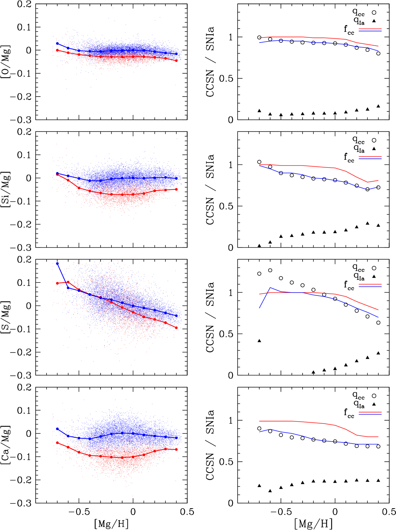
The left panels of Figure 4 show vs. distributions for other -elements (O, Si, S, Ca) in the low-Ia and high-Ia populations, with median sequences shown by connected large points. These can be compared to corresponding distributions in Figure 8 of W19, based on DR14 data; not surprisingly, the results are similar. The median [O/Mg] trends are nearly flat, with only a small separation between the low-Ia and high-Ia median sequences, as expected if the production of both O and Mg is dominated by CCSN with metallicity-independent yields. If real, the -dex separation between the sequences suggests a small contribution to O abundances from a delayed source, perhaps AGB stars rather than SNIa. For Si and Ca the sequence separations are progressively larger, implying larger SNIa contributions to these elements as predicted by nucleosynthesis models (e.g., Andrews et al. 2017; Rybizki et al. 2017). For S the two median sequences are very close, implying minimal SNIa contribution to S production, and they are sloped, implying S yields from CCSN that decrease with increasing metallicity. They diverge slightly at high , implying a growing .
The right panels of Figure 4 show the values of and derived from these median sequences via equations (26) and (25), using the ratios along the two sequences shown in Figure 1. As discussed in §2.2, with a general metallicity dependence the 2-process model fits the observed median sequences exactly; empirical evidence for the qualitative validity of the model will come from the reduction of scatter and correlations in residual abundances shown below in §5. For O the inferred at all , declining slightly at the highest metallicity. For Si and Ca the inferred values of at solar are 0.19 and 0.26, respectively. For S the low-Ia median sequence crosses above the high-Ia median sequence at low metallicity, a violation of the 2-process model assumptions that leads to slightly negative values of . Given the large observational scatter in S abundances, this sequence-crossing appears compatible with observational fluctuations, so we do not regard it as a serious problem. The inferred for S declines continuously with increasing , tracking the sloped median sequences. Because our zero-point offsets are chosen to give on the high-Ia sequence at , and because stars with have by definition, our fits always yield at (see equation 20). However, this constraint does not apply at other metallicities. Red and blue curves in these panels show the fraction of each element that is inferred to come from CCSN in stars on the low-Ia or high-Ia sequence (equation 6). Even if , the low-Ia population has at low because these stars have , implying (at least according to the 2-process model assumptions) that nearly all enrichment is from CCSN.
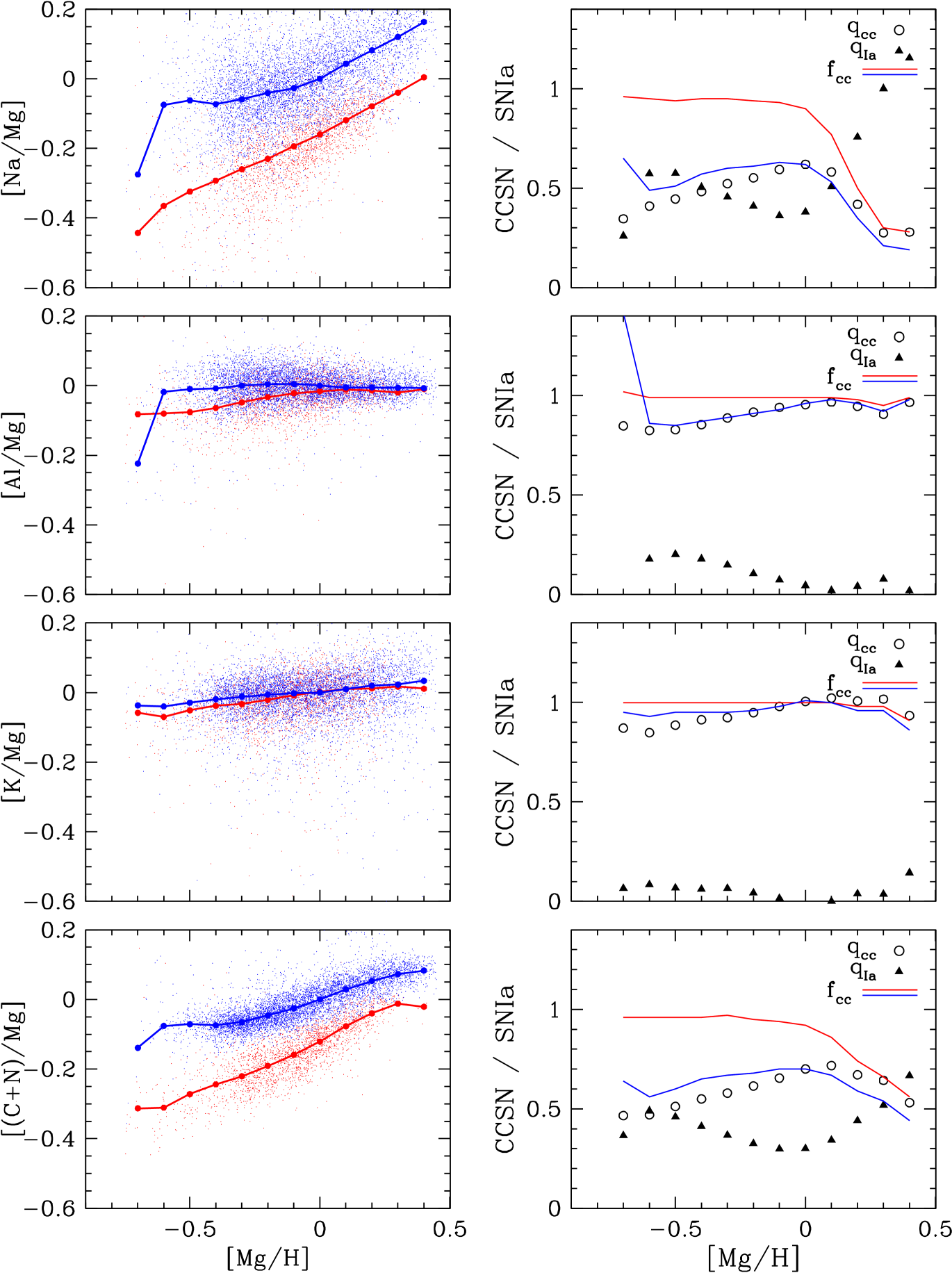
Figure 5 shows vs. distributions, median sequences, and inferred 2-process vectors for Na, Al, K, and the element combination C+N. Because they have odd atomic numbers, the nucleosynthesis of Na, Al, and K is fundamentally different from that of -elements even within massive stars. C and N are both expected to have significant contributions from AGB stars in addition to prompt contributions from CCSN and massive star winds, and the AGB yields of N are predicted to have substantial metallicity dependence (e.g., Karakas 2010; Ventura et al. 2013; Cristallo et al. 2015). Similar to W19, the median sequences for K and Al show little separation between the low-Ia and high-Ia populations, indicating a dominant contribution from CCSN; in detail, the DR17 data show a slightly larger sequence separation for Al and slightly smaller for K. More significantly, the DR17 data show [Al/Mg] trends that are essentially flat over this range while the DR14 data showed an increasing trend that implied CCSN yields increasing with metallicity.
As in W19, [Na/Mg] trends show a large separation between low-Ia and high-Ia populations implying a substantial delayed contribution to Na enrichment. Standard nucleosynthesis models predict that SNIa and AGB contributions are small compared to CCSN (Andrews et al., 2017; Rybizki et al., 2017), so this evidence for delayed enrichment comes as a surprise. The Na features in APOGEE spectra are weak, making the abundance measurements noisy and susceptible to systematic errors, but there is no obvious effect that would cause artificially boosted Na measurements at this level for high-Ia stars relative to low-Ia stars of the same . A comparable sequence separation is also found in GALAH DR2 (Griffith et al., 2019). The and values inferred from the 2-process fit are comparable in magnitude over most of the range. The inferred metallicity-dependence is complex, but given the scatter and uncertainties of the Na measurements it should be treated with caution.
While W19 considered P as an additional odd- elements, the analyses in Jönsson et al. (2020) suggest that APOGEE’s P measurements in DR16 are not robust. The P abundances are improved in DR17, but they remain subject to significant systematics, and we have elected to omit P from this paper.
The two [(C+N)/Mg] sequences show a separation nearly as large as the two [Na/Mg] sequences, again implying a substantial delayed contribution. Nucleosynthesis models predict a moderate AGB contribution to C and a dominant AGB contribution to N (Andrews et al., 2017; Rybizki et al., 2017), so this result is qualitatively expected. The inferred metallicity dependence is complex, with rising with before leveling out and dropping at high metallicity, and the opposite trend for . We caution, however, that the separation into prompt and delayed contributions is not quantitatively accurate for elements that have large AGB contributions because it is based on tracking Fe from SNIa, and the delay time distributions for AGB enrichment and SNIa enrichment are different (see, e.g., Figure 5 of Johnson & Weinberg 2020). Our present analysis does not allow us to separate the roles of C and N in these trends, though for stars with asteroseismic mass measurements one can apply corrections from stellar evolution models to infer birth abundances of the two elements (see Vincenzo et al. 2021b). The observed [(C+N)/Mg] sequences can themselves provide a quantitative test of chemical evolution models that track both elements. The high-Ia medians of [(C+N)/Mg], [Na/Mg], and [Al/Mg] all show drops in the lowest metallicity bin . This bin contains just 53 stars, so this drop could simply be a statistical fluctuation, though it might also be affected by accreted halo stars becoming a significant fraction of the high-Ia population at this low metallicity (see §7).
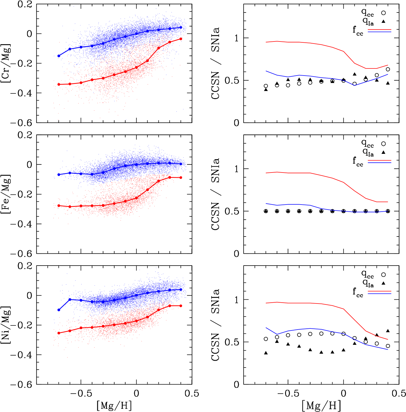
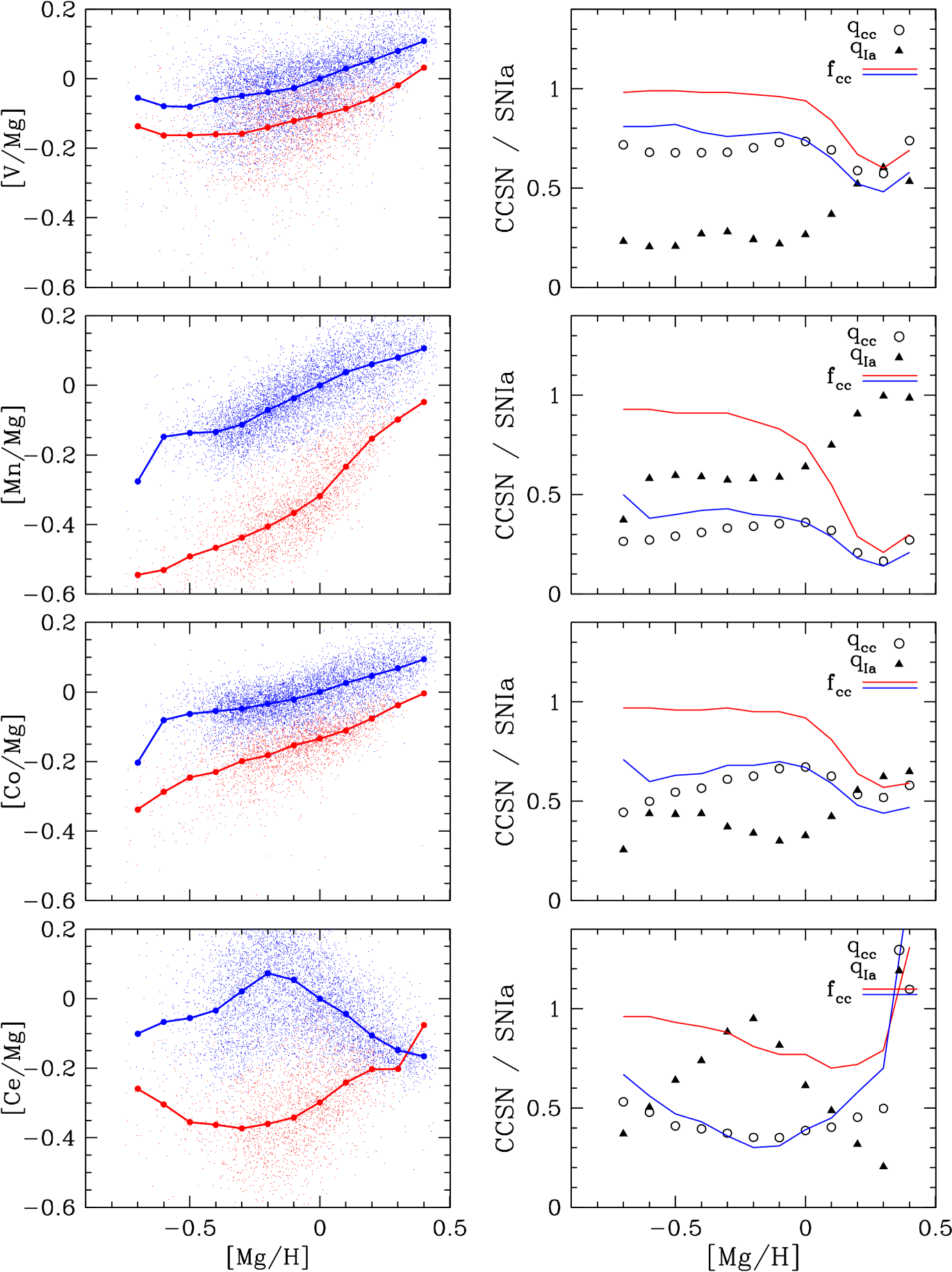
Figures 6 and 7 show sequences and 2-process parameters for iron peak elements with even atomic number (Cr, Fe, Ni) and odd atomic number (V, Mn, Co), respectively. Trends are similar to those shown for DR14 data by W19, though in W19 the trends are flatter with and the trends are steeper and with somewhat larger separation between the low-Ia and high-Ia sequences. For Fe, at all as a consequence of adopting and assuming metallicity independence. For Cr we also infer at . APOGEE Cr abundances exhibit apparent systematics for a significant fraction of stars above solar metallicity (Griffith et al., 2021a), so we regard the median sequences and inferred 2-process parameters as unreliable in the super-solar regime. While trends are similar to trends, the separation of low-Ia and high-Ia sequences is smaller, implying that CCSN contribute 60% of the Ni at solar abundances vs. 50% for iron. We find somewhat higher CCSN fractions at solar abundances for Co and V, 67% and 74%, respectively. (To phrase things still more precisely, in a star with [Fe/Mg]=[Ni/Mg]=[Co/Mg]=[V/Mg]=[Mg/H]=0, we infer that 50/60/67/74% of the star’s Fe/Ni/Co/V atoms were produced in CCSN.)
As in W19 we find that Mn has the largest SNIa contribution of any APOGEE element. Note that Bergemann et al. (2019) find a 0.15-dex difference between 1D LTE and 3D NLTE abundances from H-band Mn I lines, with little dependence on , , or ; here we take the ASPCAP Mn determinations at face value. Although the low-Ia median sequence in is steeply rising, this slope can be largely explained by the increasing SNIa enrichment fraction along the sequence, so that the inferred metallicity dependence of is weak. We infer a sharp rise in at super-solar metallicity, needed to explain the rising trend on the high-Ia sequence. Given the spectral modeling and calibration uncertainties in the super-solar regime, the rising trend of should be viewed with some caution, but it could suggest a change in the physical properties of SNIa progenitors or explosion mechanisms in super-solar stellar populations. A similar pattern of rising at is seen for C+N, Na, V, Co, and (more weakly) Ni. These common trends could indicate a delayed source (SNIa or AGB) that becomes important for all of these elements at high metallicity, though they could also be a sign that our assumptions for separating prompt and delayed components are breaking down in this regime. Like Na, Al, and C+N, the median trend of the high-Ia population drops sharply in the lowest bin for [Mn/Mg] and [Co/Mg], and to a lesser extent for [Ni/Mg].
Figure 7 also presents results for the s-process element Ce. Like Na, V, and K, APOGEE Ce abundances have relatively large statistical uncertainties (mean of 0.043 dex in our sample), and the large scatter about the median trends is likely dominated by observational errors. DR14 did not include Ce abundances, so we cannot compare to W19. However, the large separation between the low-Ia and high-Ia sequences and the non-monotonic metallicity dependence of the high-Ia sequence are qualitatively similar to results from GALAH DR2 for the neutron capture elements Y and Ba (Griffith et al., 2019). A rising-then-falling metallicity dependence is expected for AGB nucleosynthesis of heavy s-process elements: at low [Fe/H] the number of seeds available for neutron capture increases with increasing metallicity, but at high [Fe/H] the number of neutrons per seed becomes too low to produce the heavier s-process elements (Gallino et al., 1998). As with C+N, the decomposition into prompt and delayed components implied by the and values should be regarded as qualitative because the delay time distribution for AGB Ce production should differ from that of SNIa Fe production.
We report the values of and for all elements in Tables 4 and 5 in the Appendix , along with the values of along the two median sequences (Table 6). The value of follows from equation (13). These quantities can be used in equation (20) to exactly reproduce the median sequences shown in Figures 4-7. The values of (equation 8) can be used to correct observed solar abundances to the abundances produced by CCSN, which can then be used to test the predictions of supernova models, as done by W19 (their fig. 20), by Griffith et al. (2019) (their fig. 17), and most comprehensively by Griffith et al. (2021b), who carefully investigate the interplay between IMF-averaged supernova yields and black hole formation scenarios. The solar values of can be similarly used as a test of SNIa yield models, a task we defer to future work.
5 Residual abundances and their correlations
With the 2-process vectors determined by fitting the median sequences of the low-Ia and high-Ia populations, we proceed to fit the values of and for all individual sample stars as described in §2.3. We perform a -minimization fit to the abundances , [O/H], [Si/H], [Ca/H], [Fe/H], and [Ni/H], using the reported ASPCAP observational uncertainties for each measurement. We choose these six elements because they have small mean observational uncertainties, ranging from 0.0084 dex (Fe) to 0.0136 dex (Ca), because they have no major known systematic uncertainties in APOGEE data, because the production of these elements is theoretically expected to be dominated by CCSN and SNIa, and because their ratios span a wide range, giving strong collective leverage on and . The only other abundance with a mean observational error in this range is [(C+N)/Mg], but we do not use this quantity in our fits because it does not represent a single element and because the production of C and (especially) N is expected to have significant AGB contributions. The [Mn/H] abundance also has a small mean observational uncertainty (0.0144 dex), but the strong and unusual metallicity dependence of above could distort inferred ratios in this regime if it is incorrect. The 2-process amplitudes inferred from this six-element fit are close to those inferred from and alone via equations (13) and (18), but they have smaller statistical uncertainties, are robust to observational errors in these two abundances alone, and mitigate artificial correlations among residual abundances from measurement aberration (see Fig. 15 below).
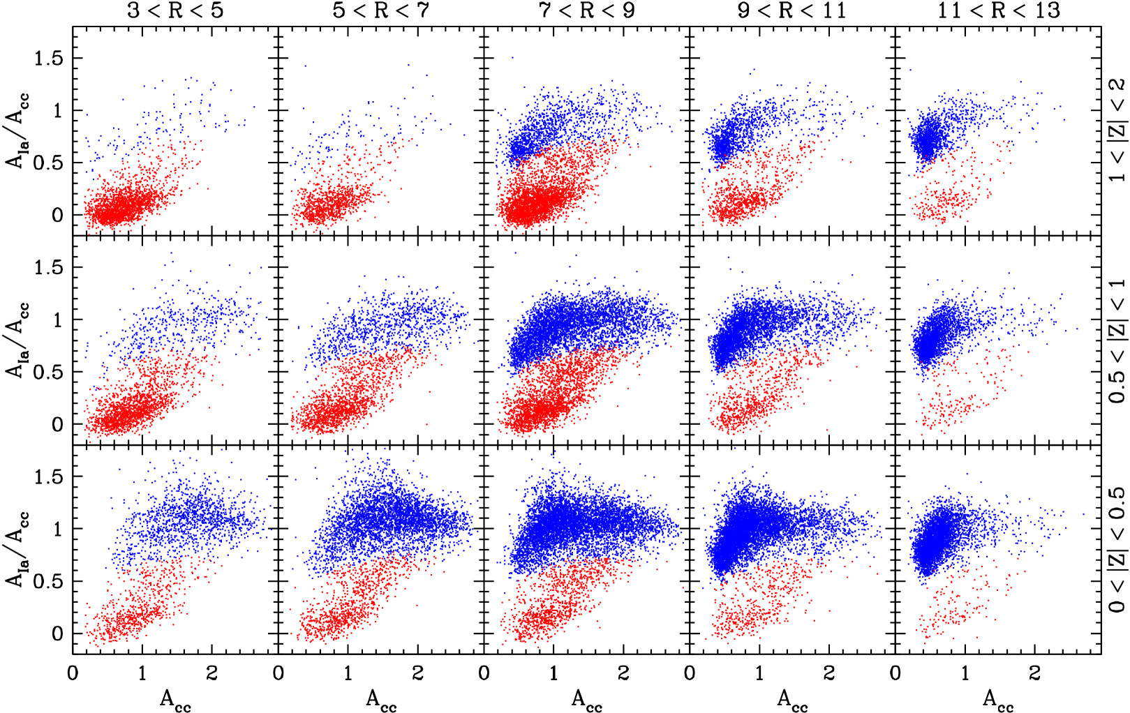
Figure 8 plots the distribution of stars in the plane of vs. in zones of Galactic and , with red and blue points denoting stars in the low-Ia and high-Ia populations, respectively. For this plot we have used our SN100 sample to improve coverage of the inner Galaxy. Although we use our six-element fits for and , this map does not look noticeably different if we use the values inferred from and alone. The -axis quantity is simply a linear measure of metallicity as traced by CCSN elements, in solar units. This plot is analogous to Figure 4 of H15, showing vs. , and still more closely analogous to Figure 3 of W19, showing vs. . Similar to those element-ratio maps, the low-Ia population is more prominent at small and large , and the metallicity () distribution of the high-Ia population shifts towards lower values at larger . However, the non-linear relations between and (equation 13) and between and (equation 18) highlight three features that are less obvious in these earlier maps. First, the median trend of in the low-Ia population rises continuously and approximately linearly with up to , reaching . Second, for the high-Ia stars also show a clear trend of increasing with , especially evident in the annuli. Both of these trends follow from the fact that the low-Ia and high-Ia sequences in are sloped below (see Fig. 1), and their persistence in a plot based on six-element fits implies that these slopes are not caused by vagaries of abundance ratio measurements. Third, the -dex scatter of along the low-Ia and high-Ia sequences, which is dominated by intrinsic scatter rather than measurement noise (Bertran de Lis et al., 2016; Vincenzo et al., 2021a), translates to substantial scatter in at a given metallicity within each population. In the solar annulus () the distribution of is clearly bimodal at sub-solar metallicity, with typical values of for the low-Ia population and for the high-Ia population. This bimodality reflects the bimodality of values, which Vincenzo et al. (2021a) demonstrate is an intrinsic feature of the underlying stellar populations that is robust to -dependent and age-dependent selection effects in the APOGEE sample.
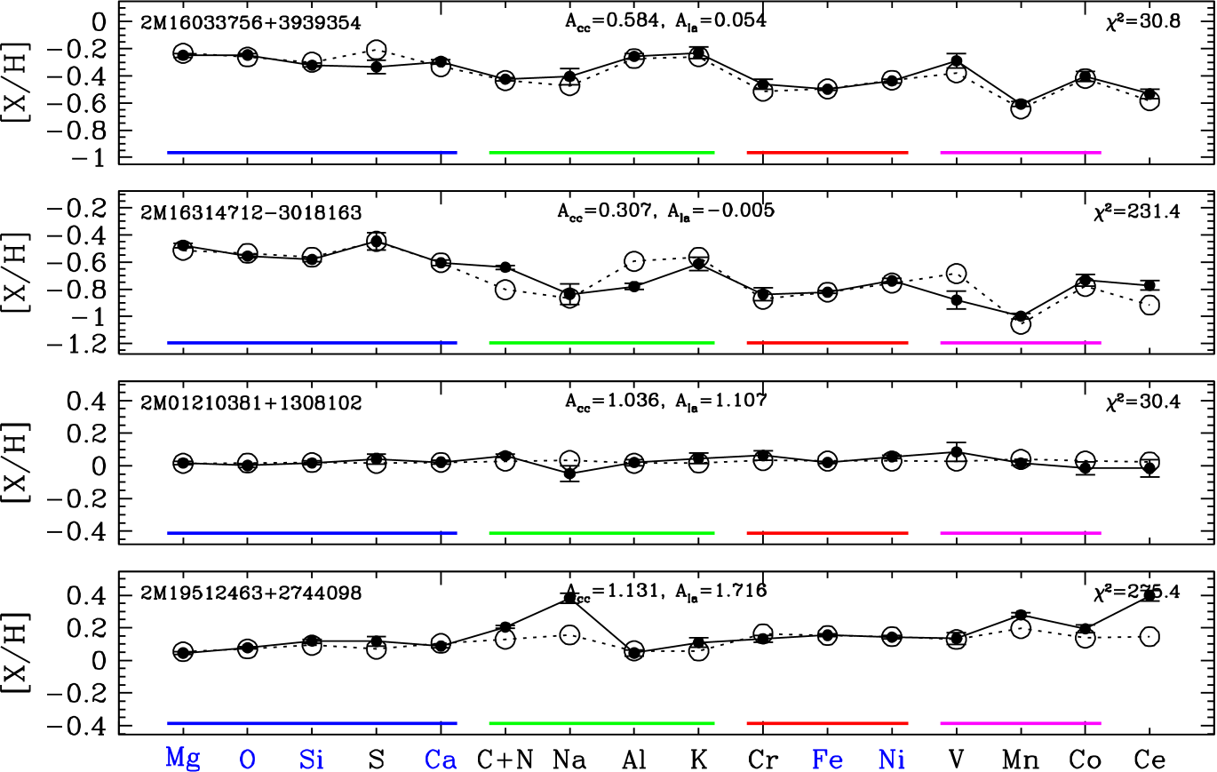
Turning to residual abundances, Figure 9 shows examples of measured vs. predicted abundances for four stars. Recall that for each sample star we fit the two free parameters and using the measured abundances of six elements, then predict all of the abundances using these two process amplitudes and the global values of and that have been inferred from the median trends of the full sample. The first two stars in Figure 9 are low metallicity members ( and 0.307) of the low-Ia population ( and -0.005), one with a value near the median for all sample stars and one with a high value near the 98th-percentile of the distribution. (Negative values can arise for stars with values above the low metallicity plateau.) The third and fourth stars are solar metallicity (, 1.131) stars from the high-Ia population, again one that is near the median of the distribution and one near the 98th-percentile.
For the first star, the 2-process model reproduces the observed abundance pattern quite well, though the value of 30.8 for 14 degrees of freedom (16 elements fit with two free parameters) is inconsistent with a purely statistical fluctuation for Gaussian measurement errors with the reported observational uncertainties. The largest residuals are for S (0.13 dex), V (0.09 dex), Na (0.07 dex), and Cr (0.05 dex), elements with relatively large observational uncertainties in APOGEE. The second star shows -dex residuals for several elements, including C+N, Al, V, and Ce, some overpredicted and some underpredicted. The predicted abundances of the third star are all nearly solar, since , and the observed abundances are also near solar, with the largest residual being 0.08 dex for Na. The fourth star shows large residuals ( dex) for Na and Ce and smaller ( dex) but statistically significant residuals for C+N and Mn. We will discuss other examples of high- outliers in §6.
5.1 Removing trends with
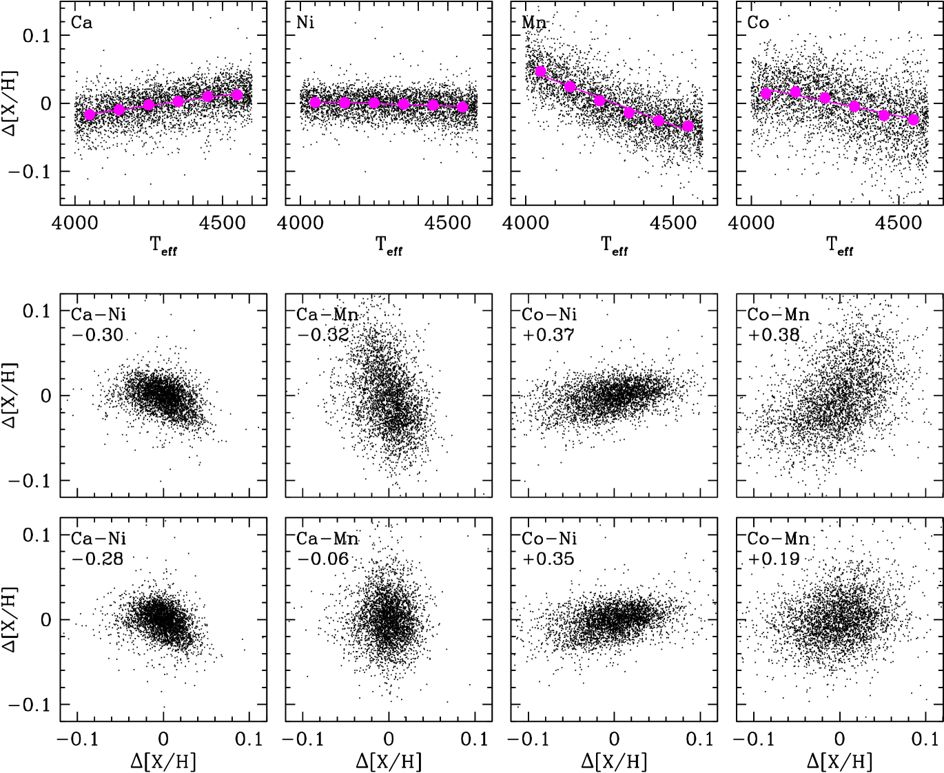
We have limited the range of and in our sample in order to minimize the differential impact of abundance measurement systematics on our results. Nonetheless, there are subtle trends of residual abundances with over this range, as illustrated for four elements in the top row of Figure 10. In this and all subsequent plots we adopt the sign convention
| (29) |
Mn residuals have the strongest trend, with the median abundance residual changing from to as increases from to . Co residuals have a weaker trend of the same sign, Ca residuals have a trend of similar magnitude but opposite sign, and Ni residuals have almost no trend with .
To avoid artificial correlations induced by these trends, we fit them with linear relations and apply corrections to the DR17 APOGEE abundance values:
| (30) |
The values of the zero-point offsets (discussed in §3) and the slopes are listed in Table 1, with values of the latter ranging from (Mg, O, K, Fe, Ni) to (Ca, Na, Al, V, Mn, Co). For Mn, for example, all abundances are increased by 0.002 dex, and the abundances of stars with are further increased by dex, thus increasing the median residual abundance to near zero. We have confirmed that residual trends with and are negligible for all elements after applying these corrections. Note that the abundances plotted in Figures 4-7 include the zero-point offsets but do not have the corrections applied. Median sequences and derived and values are negligibly affected by these trends. They matter for our subsequent analysis (and are used in all subsequent calculations and plots) because they can affect correlations of residual abundances.
The lower half of Figure 10 shows scatterplots of residual abundances for four pairs of these four abundances before (middle row) and after (bottom row) removing the trends. The Ca-Ni correlation is minimally affected because Ni residuals have almost no trend with . The correlation coefficient changes from before correction to after correction. However, Ca and Mn residuals have significant and opposite trends with before correction, causing an artificial anti-correlation with coefficient that is almost entirely removed by the correction. The Co-Ni correlation, like Ca-Ni, is minimally affected by trends. However, the Mn-Co correlation is artificially boosted because residuals of both elements are anti-correlated with , and correcting the trend lowers the correlation coefficient from 0.38 to 0.19.
In sum, we apply small (-dex) detrending corrections to the ASPCAP abundances that remove weak correlations between residual abundances and .
5.2 Simulating the impact of observational errors
If all stars were perfectly described by the 2-process model, the measured abundances would still depart from the predicted abundances because of statistical errors induced by observational noise. It is tricky to predict the distribution and correlation of these noise-induced residuals because the observational uncertainties span a significant range from star-to-star and element-to-element and because some of the measured values are used to fit the 2-process amplitudes and . We have therefore created a simulated data set in which we take each star from the sample, set its true abundances exactly equal to the 2-process predictions given its measured and , then add an “observational” error to each abundance, drawn from a Gaussian distribution with the star’s ASPCAP uncertainty for that element. If an abundance measurement is flagged in the APOGEE data, then we flag it in the simulation as well. We can then apply the same analysis to the simulated data that we apply to our observed sample to understand the results that would be expected if all stars followed the 2-process model and all measurement errors were described by Gaussian noise with the reported observational uncertainties.
5.3 Distribution of residuals
The black curve in Figure 11 shows the cumulative distribution of values for the 34,410 sample stars, computed using all of the elements shown in Figure 9 but omitting flagged element values. The median, 95th, and 99th-percentiles of this distribution are 30, 134, and 438, respectively. Only 13% of stars have values below 14, the number of degrees of freedom for 16 elements and two free parameters, so either the true distribution has intrinsic element scatter relative to the 2-process model or the observational abundance errors exceed those predicted for Gaussian noise with the ASPCAP uncertainties, or both. The red curve shows the distribution for the simulated data set described in §5.2, and in this case 45% of stars have .
The green curve shows the distribution if and are inferred from [Mg/H] and [Fe/Mg] alone instead of the six-element 2-process fit. This leads to only a small increase in values. The blue curve shows the distribution of if we compute element residuals from the observed median sequences instead of the 2-process fits, interpolating the sequences in to avoid any effects of metallicity variation across our 0.1-dex bins. These values are substantially higher (e.g., a median value of 78, vs. 30 for the 2-process residuals), a first demonstration that the 2-process model is removing physical scatter present in the stellar abundance distribution. In other words, a star’s APOGEE abundances are typically closer to those predicted by the 2-process model than they are to the median abundances of stars of the same and the same population (low-Ia or high-Ia), by an amount that is highly statistically significant.
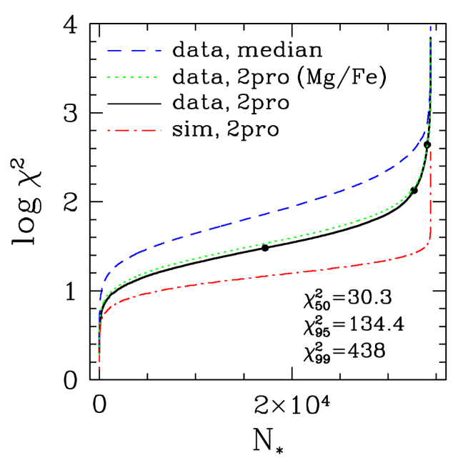
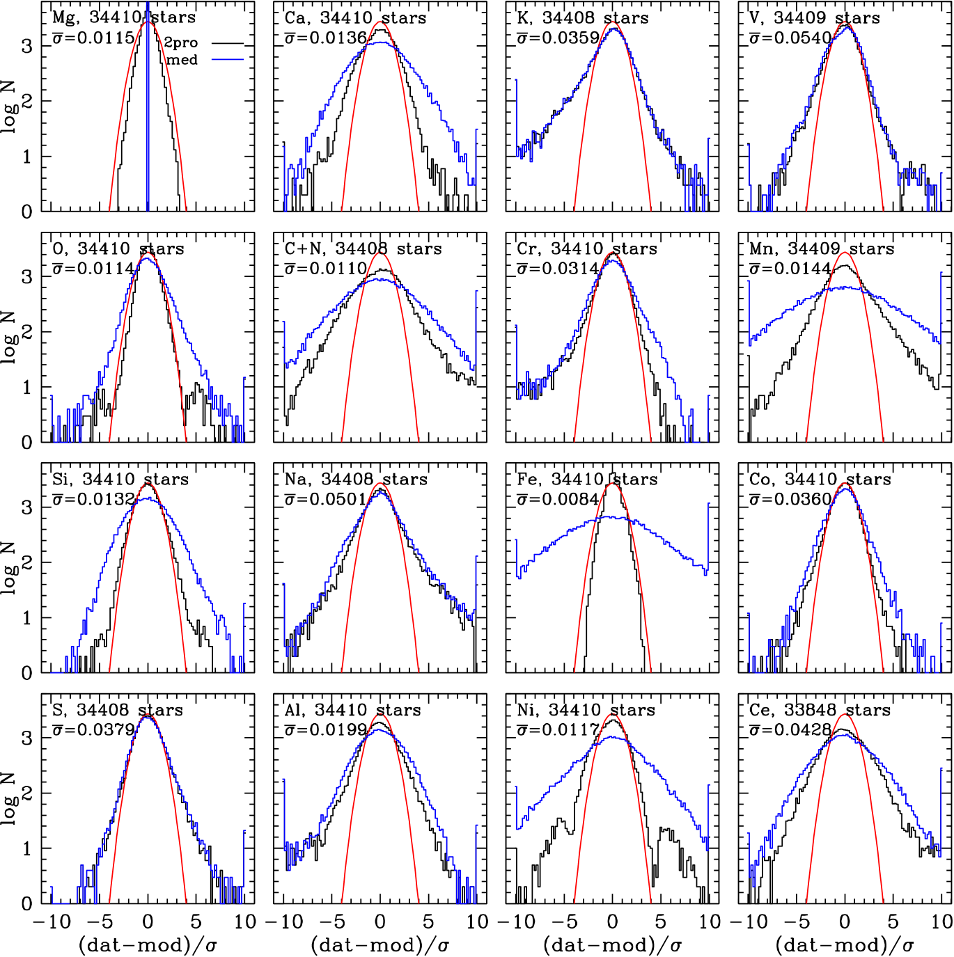
Figure 12 examines the deviation distributions element-by-element. For those elements that have a mean ASPCAP abundance error smaller than 0.015 dex, the deviations from the 2-process model predictions (black histograms) are significantly narrower than the deviations from the median sequence predictions (blue). Some of this improvement arises because many of these elements are used in the 2-process fit, but even if we use only Mg and Fe to determine the 2-process parameters the deviation distributions for the other fit elements are narrower than the distribution of deviations from the median sequences. Mn and C+N, which are not used in the 2-process fit, both show narrower deviations from the 2-process predictions than from the median sequences. For other elements, with larger mean errors, there are only small differences between the 2-process deviation distribution and the median-sequence deviation distribution, presumably because the deviations in both cases are dominated by observational errors. However, the extended tails of the distributions are still noticeably reduced for Al, Cr, Co, and Ce.
Red curves show a unit Gaussian, which is narrower than the 2-process deviation distributions for all elements except Mg and Fe. The simulated star sample drawn from the 2-process model yields deviation distributions (not shown) very close to these unit Gaussians, as expected. For many elements the extended tails of the deviation distribution appear more nearly exponential than Gaussian, and for some elements there is a significant asymmetry between positive and negative deviations in these extended tails. Extended tails and asymmetries could arise from either genuine physical deviations or measurement errors. We investigate this question to a limited degree in §6, though it is difficult to quantify the relative contribution of physical and observational outliers without detailed investigation of the abundance determinations for a large number of stars.
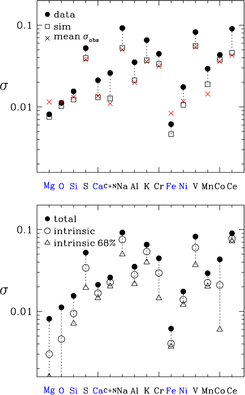
In both panels of Figure 13, filled circles show the rms difference between ASPCAP abundances and 2-process model predictions. In the upper panel, red crosses show the mean abundance error reported by ASPCAP for that element. Open squares show the rms deviations for the simulated data set. These simulated dispersions are generally very similar to the mean abundance errors, though they are significantly lower for Mg and Fe, which carry high weight in the 2-process fit. In the lower panel, we estimate the intrinsic dispersion by subtracting the dispersion of the simulated data from the dispersion of the observational data. If intrinsic and observational scatter contributed equally to the variance, then the intrinsic dispersion would be of the total dispersion. Half of the elements have an intrinsic/total dispersion ratio near or below this value (Mg, O, Si, S, Cr, Fe, V, Co), and the other half have higher ratios that imply intrinsic dispersion dominating over the observational scatter. However, the observational contribution could be underestimated, and the intrinsic dispersion overestimated, if the reported measurement uncertainties are systematically low or if non-Gaussian tails of the measurement errors inflate the dispersion. As already noted, the residual distributions for many elements exhibit exponential tails, which could represent real deviations or non-Gaussian measurement errors. As an alternative estimate of dispersion, we have taken half of the 16-84% percentile range ( for a Gaussian distribution) for the observed residuals, then computed the same quantity for the simulated data and subtracted in quadrature, obtaining the open triangles in Figure 13. These alternative estimates characterize scatter in the core of the residual abundance distribution, with less sensitivity to large deviations (whether physical or observational).
For Mg, O, and Fe we estimate rms intrinsic scatter of only 0.003-0.005 dex, but given the weight of these elements in the 2-process fit a low scatter is expected. For other elements the rms intrinsic scatter ranges from dex (Si, Ca, C+N, Ni, Mn, Co) to dex (Na, K, V, Ce). The percentile-based intinsic scatter estimate is lower for all elements, with Mg, O, Si, S, Ca, C+N, Al, Cr, Fe, Ni, Mn, and Co having values dex and the Na, K, V, and Ce scatter reduced to 0.04-0.07 dex. Our estimates of intrinsic scatter, including the relative values of different elements, are similar to those inferred by TW21 for scatter in APOGEE abundances conditioned on [Mg/H] and [Mg/Fe]. We originally performed our analysis for the APOGEE DR16 data set, and while the relative ranking of elements was nearly the same, the total scatter and estimated intrinsic scatter were consistently higher. The lower estimates of intrinsic scatter in DR17 likely reflect improvements in the abundance analysis that reduce the number of large measurement errors.
In sum, the 2-process model predicts a star’s APOGEE abundances better than the median abundances of similar stars, demonstrating that much of the abundance scatter within the low-Ia and high-Ia populations arises from scatter in SNIa/CCSN ratios at fixed . RMS residuals about 2-process predictions range from dex for the most precisely measured elements to dex for Na, V, and Ce. These dispersions exceed those expected from observational errors alone, implying intrinsic scatter at the dex level, depending on element.
5.4 Covariance of residuals
As emphasized by TW21, correlations are a more robust measure of residual structure in elemental abundance patterns than dispersion, because estimating the intrinsic dispersion requires accurate knowledge of the observational error distribution. The correlations also provide richer information about the sources of residual structure, which could include additional enrichment processes, stochastic sampling of the IMF, binary mass transfer, or even effects like variable depletion of refractory elements in proto-planetary disks or abundances boosted by giant planet engulfment. We compute elements of the covariance matrix of element pairs Xi, Xj as
| (31) |
with defined as the difference between the observed abundance and the 2-process model prediction (equation 29).
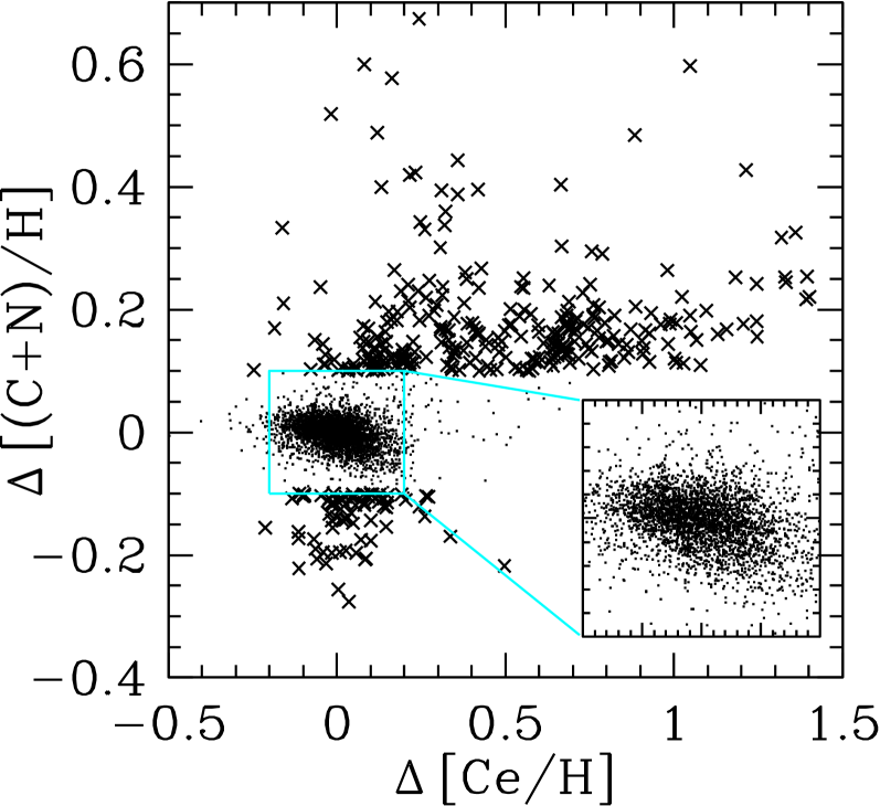
Pairwise scatterplots of element residuals generally resemble the examples shown in Figure 10. In particular, for element pairs with significant correlation or anti-correlation, the scatterplot shows a consistent slope between the core of the distribution and the stars with large residuals. The one exception is (C+N) vs. Ce: the core of the distribution shows a clear anti-correlation of the residual abundances, but there is a population of rare outlier stars with large positive residuals in both (C+N) and Ce, as illustrated in Figure 14. We discuss this population further in §6. To avoid covariance estimates being driven by rare outliers, we eliminate stars with element deviations before computing covariances involving that element. This censoring reverses the sign of the (C+N)-Ce covariance, which would be positive instead of negative if we retained the extreme outliers. It has a moderate impact on some other matrix elements involving Ce or (C+N) and minimal effect on other element pairs.
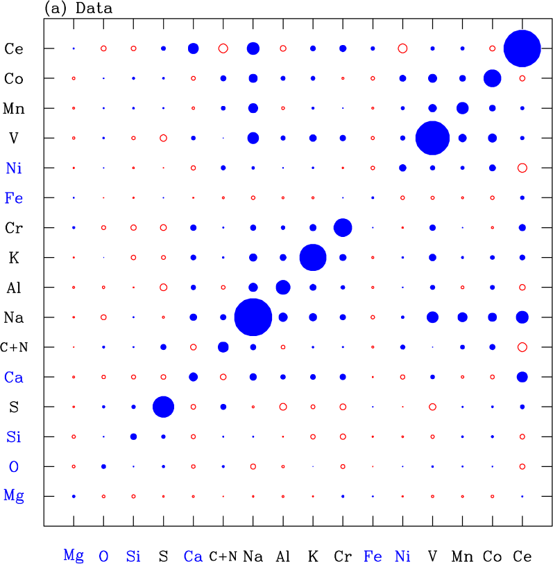
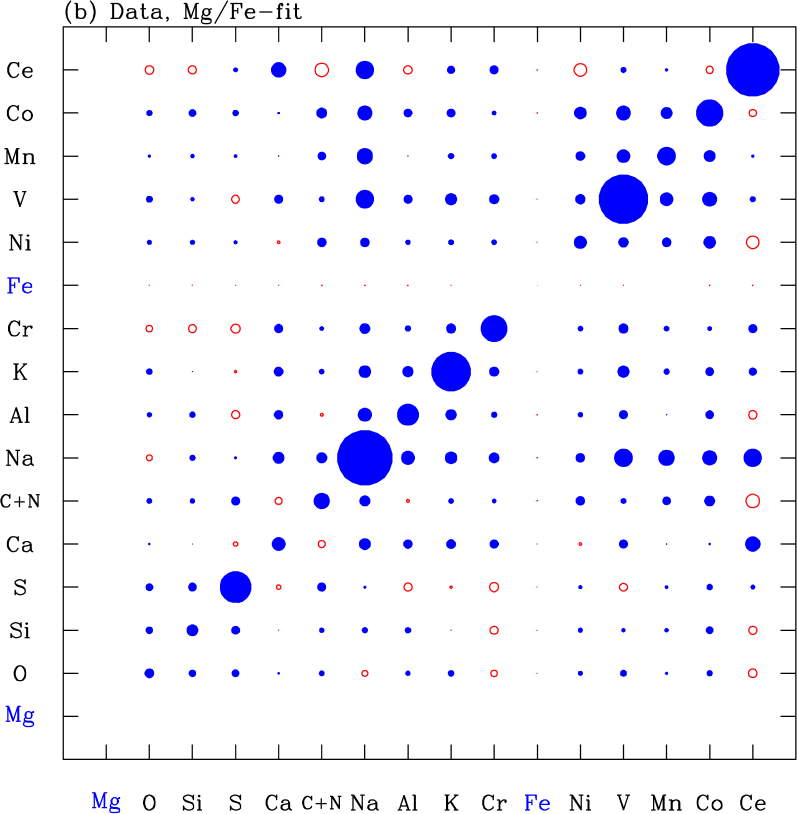
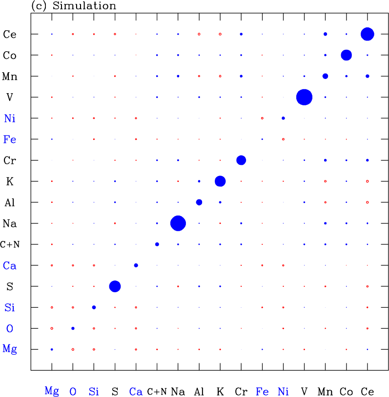
Figure 15a shows the residual abundance covariance matrix of our APOGEE sample. Diagonal elements are the squares of the rms deviations shown by the filled circles in Figure 13. This covariance matrix would look qualitatively similar if we did not remove the temperature trends discussed in §5.1, but the covariances involving pairs of elements with the strongest trends (largest values of in Table 1) would be noticeably affected. Figure 15b shows the residual covariance if we determine and values from [Mg/H] and [Mg/Fe] alone, instead of fitting six elements. Here the correlations are stronger and almost all positive, except those involving Mg and Fe, which have vanishing residuals by definition. These artificial correlations span many elements because random Fe and Mg measurement errors lead to errors in and and thus to correlated deviations from the 2-process predictions, the effect that TW21 describe as “measurement aberration.” Fitting six elements mitigates this effect, though it does not entirely remove it. Figure 15c shows the covariance of the simulated data, which has no intrinsic residual correlations by construction. However, because and must be fit to abundances with random statistical errors, measurement aberration still produces off-diagonal covariances.
The most important conclusion from comparing the simulation covariance matrix to the data covariance matrix is that measurement aberration is much too small to explain the observed covariances. Our conclusion agrees with that of TW21, who investigated the correlation of residual abundances in the conditional probability distribution at fixed and , using an APOGEE sample nearly identical to ours. TW21 also find that the measured residual correlations are much larger than those arising from measurement aberration. Artificial correlations could also arise from the abundance determination itself, e.g., from random errors in leading to correlated deviations in the abundances of multiple elements. TW21 examine this issue by approximately modeling the ASPCAP measurement procedure and conclude that artificial correlations from the measurement method are also much smaller than the observed correlations (see their figure 9).
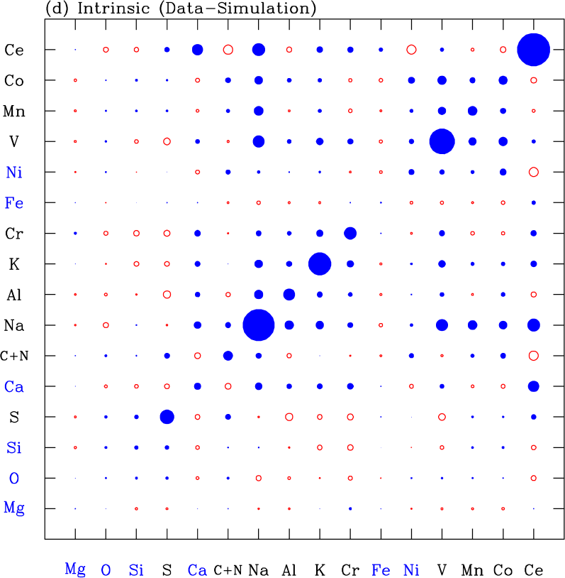
To estimate the covariance matrix of intrinsic deviations from the 2-process model, we subtract the simulated covariance matrix (c) from the data covariance matrix (a). This subtraction produces little change because the elements for the simulation are generally much smaller than those of the data. The result is shown in Figure 15(d). The diagonal elements of this covariance matrix correspond to the open circles in Figure 13. As discussed in §5.3, the estimates of the intrinsic variance are sensitive to knowledge of the observational error distribution, so their magnitudes are uncertain. However, the prominent off-diagonal structures in §5.3 likely represent genuine physical correlations among abundance residuals. The most obvious of these structures are the block of correlations among the iron-peak elements Ni, V, Mn, and Co, and another block of correlations among the elements Ca, Na, Al, K, and Cr. Ce is also positively correlated with all members of this latter group except Al. There is also a noticeable positive correlation of Na with V, Mn, and Co.
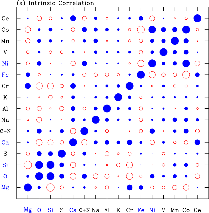
Figure 16a converts this intrinsic covariance matrix to the corresponding correlation matrix,
| (32) |
thus normalizing all diagonal elements to unity. This transformation depends on our estimate of the intrinsic variance, and if we used the percentile-based estimates (triangles in Figure 13) then the off-diagonal correlations would all be larger, though the structure would be similar. Relative to the covariance matrix, this conversion highlights the substantial correlations among elements that have small observational and total scatter. The intrinsic correlation matrix is similar in its main features to that found by TW21 (see their figure 10), including the previously noted correlations among the iron-peak element residuals, positive correlations among O, Si, and S, and positive correlations among Ca, Na, and Al (extending here to include K and Cr). Since conditioning on Mg and Fe has much in common with fitting the 2-process model, we would expect residual correlations to be similar, but details of our analysis are entirely different and independent, so we consider this agreement an encouraging indication that the correlations are qualitatively robust to these details. Many of these correlations are quite strong, e.g. 0.15 or larger, and would be stronger still if we used the percentile-based intrinsic variance estimate.
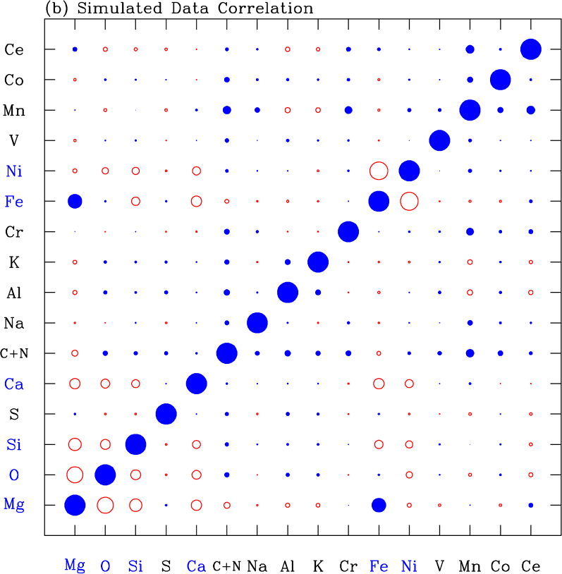
Figure 16b shows the correlations for the simulated data set. This shows that measurement aberration can induce substantial spurious correlations even with six-element fitting. The primary effects are a positive correlation between Mg and Fe and anti-correlations between these elements and the other fit elements (O, Si, Ca, Ni), and to a lesser degree among those elements themselves. In principle our subtraction of the simulated covariance matrix from the data covariance matrix should have removed these artificial correlations from our estimate of the intrinsic correlation matrix. However, given the uncertainties in this procedure (primarily our imperfect knowledge of the observational error distributions), the inferred correlations involving the fit elements should be treated with some caution. If we used only Mg and Fe to infer and , then the off-diagonal correlations for the simulated data set would be comparable in typical magnitude but nearly all positive.
In sum, the measured covariance of residual abundances is larger than expected from observational errors alone, demonstrating the existence of intrinsic physical correlations in the residual abundance patterns. The most prominent of these are correlations among Ca, Na, Al, K, Cr, and Ce and correlations among Ni, V, Mn, and Co.
5.5 Correlations with age and kinematics
Figure 17 plots the amplitude ratio inferred from our 2-process fits against the stellar age inferred from the APOGEE spectra by AstroNN (Leung & Bovy, 2019b; Mackereth et al., 2019), a Bayesian neural network model trained on a subset of APOGEE stars with asteroseismic ages. We use the DR17 AstroNN Value Added Catalog, which will be made available with the DR17 public release. Specifically we use the age_lowess_correct ages, which correct the raw neural network ages for biases at low and high age using a lowess smoothing regression (see Mackereth et al. 2017). We adopt the same Galactic zones shown previously in Figure 8 and again use the SN100 sample to improve coverage of the inner Galaxy. In the solar neighborhood (, ) we compute the median age in narrow bins of , and we repeat this median sequence in other panels for visual reference. We use this order of binning because is measured much more precisely than age, so the median in bins of age cannot be determined as reliably.
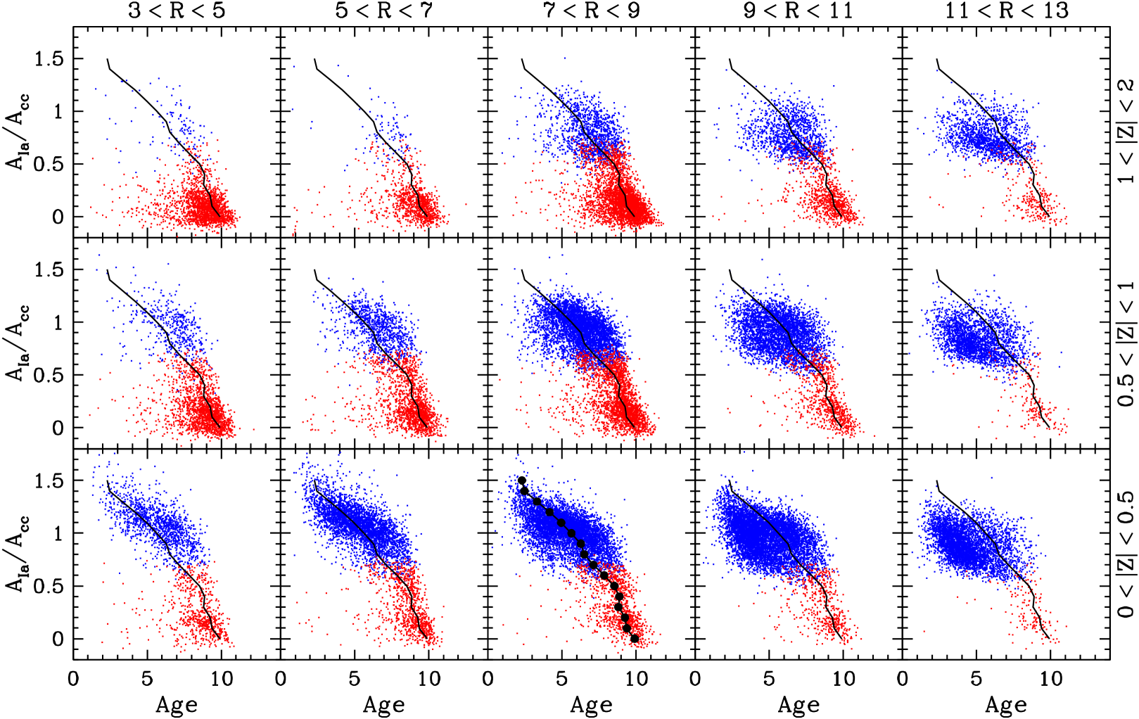
Not surprisingly, the low-Ia stars are systematically older than the high-Ia stars. There is, furthermore, a continuous trend of age with within both the low-Ia and high-Ia populations, and although these two populations are separated in the age trend is continuous across them. The trend is similar in different Galactic zones, though in the high-Ia population at the stars are systematically older in the inner Galaxy and younger in the outer Galaxy at fixed , by roughly 1-2 Gyr. The correlation of age with within the high-Ia population is visible in previous studies (Martig et al., 2016; Miglio et al., 2021), though it is perhaps more obvious in this representation.
The primary spectroscopic diagnostic of age in APOGEE spectra comes from features that trace the C/N ratio (Masseron & Gilmore, 2015; Martig et al., 2016), because the surface C and N abundances are changed by dredge-up on the giant branch in a way that depends on stellar mass, and for red giants the age (slightly longer than the main sequence lifetime) is tightly correlated with mass. Although AstroNN works directly on spectra, it responds primarily to C and N features and returns large age uncertainties when these features are masked. It is therefore unlikely that it is “learning” a correlation between age and other abundance ratios from its asteroseismic training set and then applying that to other stars. However, the birth [C/N] ratio likely depends on stellar metallicity and [/Fe] (Vincenzo et al., 2021b), and these birth abundance trends could induce systematic age errors that correlate with abundances.
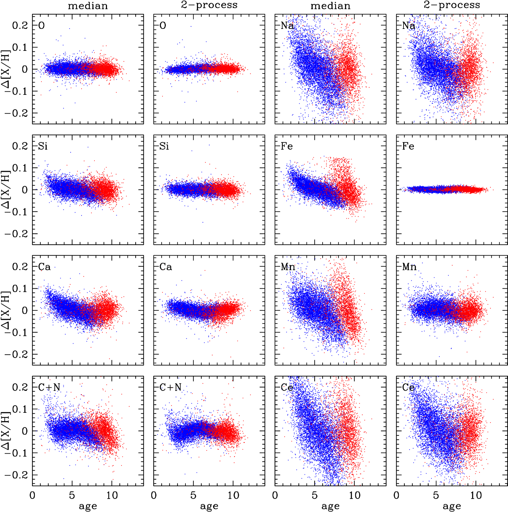
Figure 18 plots residual abundances vs. AstroNN age. We return to using the high SNR-threshold sample to reduce observational contributions to the residual scatter, and we have selected a subset of elements that illustrate a range of behaviors. In the first and third columns, is computed relative to the median sequence of the low-Ia or high-Ia population. We see a clear correlation between and age in the high-Ia population and a weaker correlation in the low-Ia population. This correlation indicates that even though the scatter about the median sequence at fixed is small (about 0.04 dex in , see Vincenzo et al. 2021a), it is correlated with age in the expected sense, with younger stars showing greater Fe enrichment. Mn, which we infer to have the largest SNIa contribution of all APOGEE elements (Figure 7), shows a similarly strong correlation, and Na and Ce show similar correlations in the high-Ia population despite the larger scatter from observational errors. O residuals show no correlation with age, but Si and Ca residuals do, consistent with our inference of a significant SNIa contribution to these two -elements (Figure 4). Residual correlations for C+N are weak, though there is a population of older high-Ia stars that have below-median C+N.
In the second and fourth columns, is computed relative to the predictions of the 2-process model. The residual scatter is smaller for the well measured elements, as seen previously in Figures 12 and 13. The age trends seen previously for Fe, Mn, and Si are removed, and the trend for Ca is reduced though not entirely eliminated. We regard this flattening of age trends as evidence for the physical validity of the 2-process model, which is constructed with no knowledge of the stellar ages. However, residuals from the 2-process model could correlate with age if they are caused by other enrichment processes that have a different time dependence than SNIa. We see a slight correlation of C+N residual with age in the high-Ia population, though there is some risk of a systematic effect because of the central role of these elements in the age determinations.
More strikingly, we see a clear trend of Ce residuals and, to a lesser extent, Na residuals with age in the high-Ia population. Stars with have typical AstroNN ages of 2-3 Gyr, while stars with have typical ages of 4-6 Gyr. Within the high-Ia population, the trend continues to negative and older ages, though there is no clear trend within the low-Ia population. These results are qualitatively consistent with the findings of Sales-Silva et al. (2021) that APOGEE’s [Ce/Fe] and [Ce/] ratios for open clusters increase with decreasing cluster age over at least the past . Previous studies (e.g., da Silva et al. 2012; Nissen 2015; Feltzing et al. 2017) have also shown that abundances of s-process elements are well correlated with age in thin-disk stars. We have already noted (§4) that the separation of median sequences for [Na/Mg] is larger than expected based on the yield models used by Andrews et al. (2017) and Rybizki et al. (2017). The qualitative similarity of age trends for Na and Ce residuals suggests that a common source, presumably AGB stars, makes important contributions to both elements.
In future work we will directly examine trends with asteroseismic ages, instead of the spectroscopic estimates trained on them. However, the current sample is not ideally suited for this purpose because our and cuts eliminate many of the APOGEE stars for which asteroseismic parameters from Kepler are available (Pinsonneault et al., 2018).
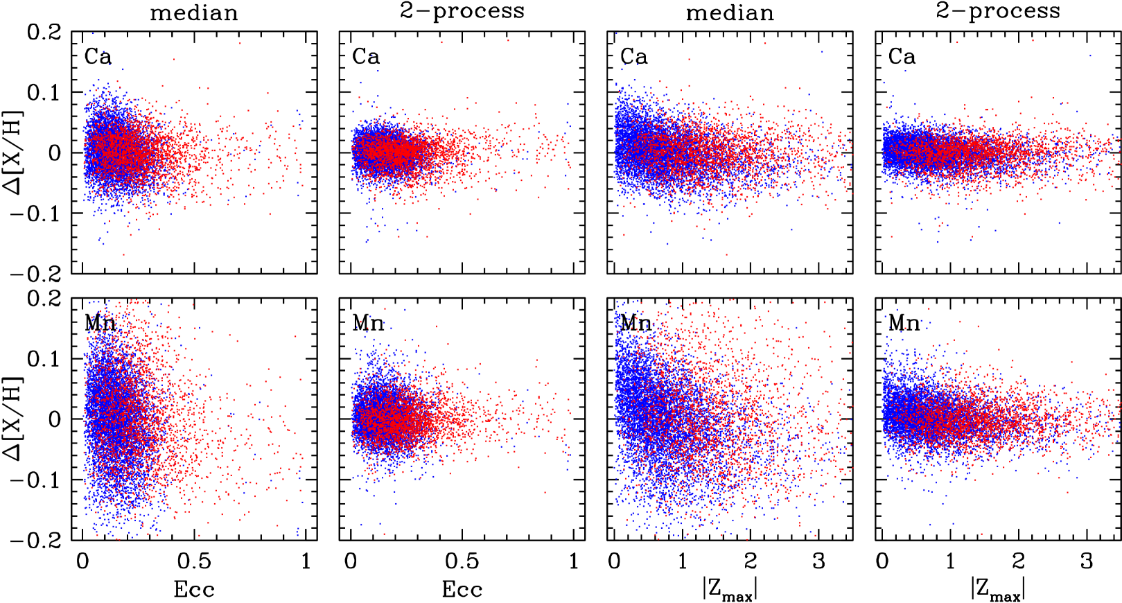
Figure 19 plots residual abundances for Ca and Mn against orbital parameters derived by AstroNN from APOGEE and Gaia data, computed using the fast method of Mackereth et al. (2018) implemented in galpy (Bovy, 2015), assuming the MWPotential2014 gravitational potential from Bovy (2015). The two left columns show residuals vs. eccentricity. Not surprisingly, low-Ia (“thick disk”) stars are more likely to have high orbital eccentricity than high-Ia stars. Within each population, there is a slight tendency for the highest eccentricity stars to have lower [Ca/H] and [Mn/H] relative to the median sequence, but this trend is weak, and it vanishes when examining residuals from the 2-process fits instead of from the median sequence. The right two columns show residuals vs. , the maximum distance a star’s orbit reaches from the midplane. Low-Ia “thick disk” stars are more likely to have high , though a number of stars in the high-Ia population have inferred . Trends (or lack thereof) are similar to those seen for eccentricity but somewhat more pronounced. In particular, high-Ia stars with tend to have higher [Ca/H] and [Mn/H] relative to the median sequences, an effect that is subtle (0.02-0.05 dex) but discernible with a large sample. The coldest “thin disk” stars tend to have higher fractions of elements with SNIa contributions, as expected from the trend of with age (Fig. 17) and the age-velocity relation.
As with eccentricity, shifting from median residuals to 2-process residuals removes these weak correlations. We have examined other elements and find no convincing correlations of individual 2-process residuals with kinematics or with Galactic position. As discussed in §8 below, grouping correlated elements sharpens sensitivity and reveals weak correlations that are difficult to discern in individual element plots like Figures 18 and 19. In §7 we give examples of stellar populations whose median residual abundances clearly depart from those of the main disk sample.
In sum, deviations from median sequences show weak but expected correlations with age and kinematics, with the stars that have higher SNIa/CCSN ratios within each population also having younger ages and colder kinematics. Changing to 2-process residuals removes most of these correlations, but within the high-Ia population the Ce and Na residuals show significant age correlations, with younger stars exhibiting higher abundances of both elements relative to stars with similar and .
6 High- Stars
The 2-process model fits the APOGEE abundances of most disk stars to an accuracy that is comparable to the reported observational uncertainties. However, the estimated intrinsic scatter about the 2-process predictions exceeds 0.01 dex for most elements (Figure 13), and the off-diagonal covariance of abundance residuals demonstrates the physical reality of intrinsic deviations even among stars that appear individually well described by the model (Figures 10 and 15). In this section we examine a selection of stars whose measured abundances are poorly described by the 2-process model, i.e., with high values of . We refer to these stars as outliers, but we note that with sufficiently precise measurements it is likely that most stars would show statistically robust deviations from the 2-process fit. Some of these outlier stars may simply be extreme examples of the same correlated deviations present in the main stellar population, offering clues to the physical drivers of these deviations. In other cases, unusual abundances may arise from rare physical processes that do not affect most stars. Yet other high- cases arise from measurement errors that are much larger than the reported observational uncertainty, for reasons that may be simple (e.g., a poorly deblended line) or subtle (e.g., inaccurate interpolations in a grid of synthetic spectra at an unusual location in abundance space).
High values can arise from single deviant measurements, which may have a variety of mundane observational causes. To preferentially select genuine physical outliers, we have used a modified criterion in which (a) we use the total scatter (filled circles in Figure 13) rather than the observational uncertainty, and (b) for each star, we omit the element that makes the single largest contribution to . This criterion thus requires at least two anomalous abundances, and it downweights the impact of elements that more frequently have observational errors much larger than the reported uncertainties. Figure 20 shows a selection of eight stars drawn from the top 2% of this modified distribution. We list both the original and the modified for each star. For reference, the 98%, 99%, and 99.5% highest values of the modified are 59.9, 97.0, and 154.7, respectively. We selected these eight stars after examining examples in the top 2%, illustrating a few of the common themes that we find within this high- population.
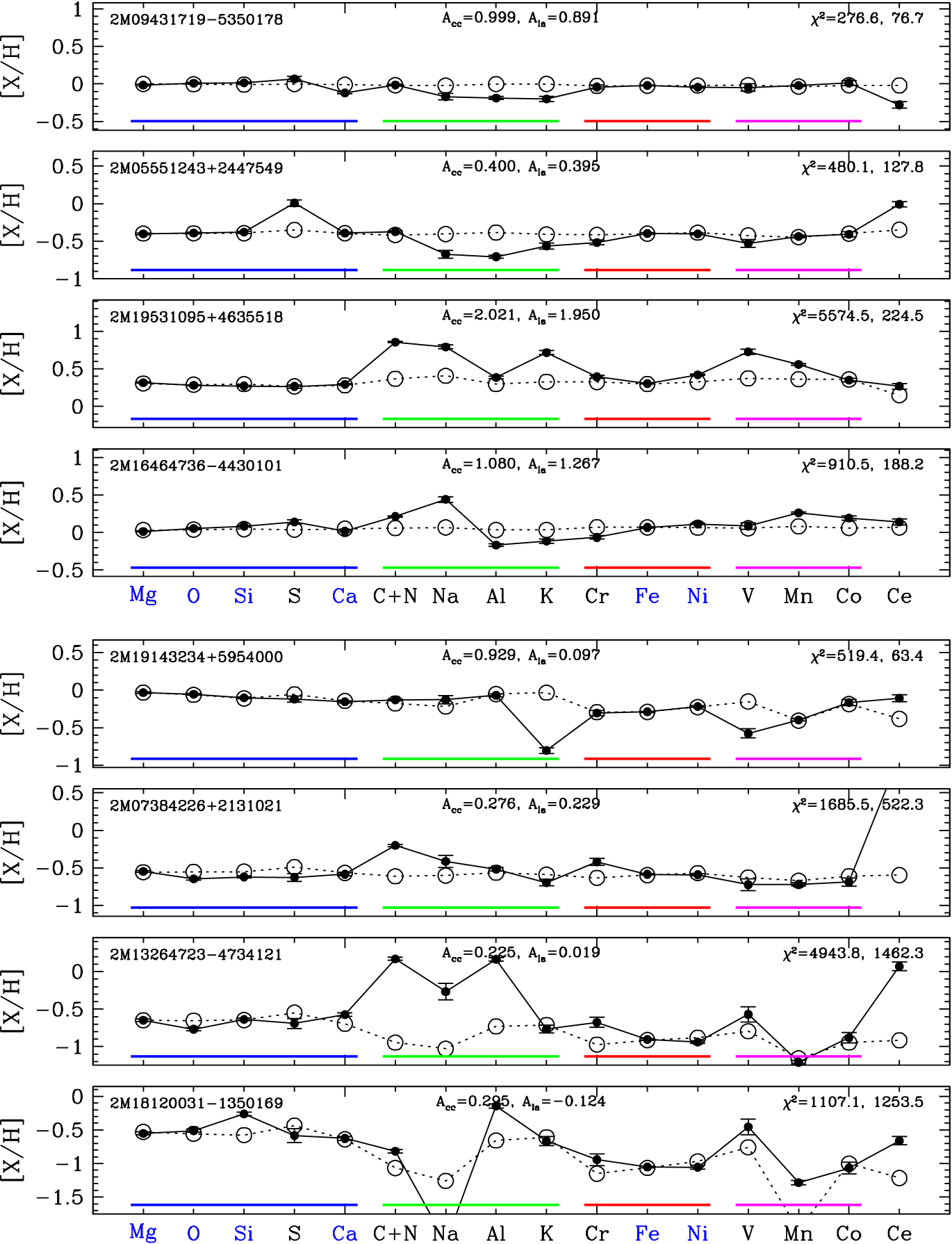
2M09431719-5350178 has nearly solar values of and , but it has low values (relative to the 2-process predictions) of Ca, Na, Al, K, and Ce, by dex for Ce and 0.1-0.2 dex for the other elements. This star individually exemplifies the pattern shown by the block of observed correlations in Figure 15d, and we find similar behavior in some other high- stars. These examples and the residual correlations themselves hint at a common physical source that contributes to these elements and is deficient in some stars. However, we do not have a clear physical interpretation of this pattern. We have not noticed comparably clean examples in which all of these elements are high, though Figure 23 (discussed in §8) shows two examples with high average deviations among these elements.
2M05551243+2447549 is a lower metallicity, high-Ia star (, ) that shows a similar deficiency of Na, Al, and K but a Ce abundance that is enhanced by 0.34 dex, demonstrating that large deviations among these elements do not necessarily move in lockstep. This star also shows a large (0.36-dex) enhancement of S relative to the predicted, near-solar [S/Mg]. This star has broader lines than the synthetic spectral fit, suggesting high rotation, and it has a radial velocity spread of over the 100 days that it was observed, implying a binary companion. While these properties could be connected to unusual abundances, it is also possible that high rotation is causing systematic errors in the ASPCAP abundance measurements, and in the spectroscopic , which is low (by about 0.4 dex) relative to most stars of similar metallicity and .
2M19531095+4635518 is a metal-rich, high-Ia star (, ) that is an extreme outlier in both its standard and its modified . This star has an extremely high C+N residual, with ASPCAP values of [C/Fe]=0.32 and [N/Fe]=1.04. The [O/Fe] from ASPCAP is 0.045, implying a C/O number ratio of 1.01 that puts this star just over the boundary into the carbon star regime, where the stellar spectral features become very different from those of typical, stars. The large deviations in Na, K, V, and Mn may be physical, but they could also be affected by the very strong blends that occur in the carbon star regime, such that any inaccuracies in the ASPCAP synthesis could lead to poor fits or incorrect abundance values.
2M16464736-4430101 displays a pattern that we have found in multiple examples of high- stars of solar or super-solar metallicity. Consistently in these stars, the Na abundance is far above the 2-process prediction (by 0.37 dex in this case), the C+N abundance is moderately elevated ( dex), the Al, K, and Cr abundances are moderately depressed, and the V, Mn, and Co abundances are slightly enhanced. Although this could be a distinctive class of chemically peculiar stars, we suspect that this pattern arises from an artifact of ASPCAP abundance determinations, in part because we find anomalous structures in [X/Fe]-[Fe/H] diagrams for Na, Al, and Mn that do not appear physical. We do not understand the origin of this artifact, though the elevated C+N hints that it could be related to inaccurate interpolation across the model grid near the carbon-star regime, where spectral syntheses change rapidly with stellar parameters.
2M19143234+5954000 has near-solar and an that places it below the median of the low-Ia population at this metallicity (Figure 6). Its high value is driven by extremely low K and low V, and to a lesser extent by elevated Ce. Low K values and to some degree low V values are fairly common among high- stars, and the residual distributions for both elements (especially K) are asymmetric towards negative values (Figure 12). K and V both have weak, sometimes blended features in APOGEE spectra, so the abundances are more subject to statistical and systematic errors. Furthermore, follow-up of the low K population shows that many of them (including this star) have a heliocentric velocity of that happens to place two of APOGEE’s K lines on top of stronger telluric features. It therefore seems likely that the low K abundances are a consequence of imperfect telluric subtraction.
2M07384226+2131021 is a low metallicity,444We refer to stars with as low metallicity because they lie at the metal poor end of our sample and of disk populations in general, though of course halo populations reach to much lower metallicity. high-Ia star (, ) with highly elevated C+N (0.41 dex) and extremely elevated Ce (1.59 dex), as well as moderate enhancements ( dex) in Na and Cr. This star is a member of the old open cluster NGC 2420, and it was identified by Smith & Suntzeff (1987) as an extreme example of a “barium star” based on its strong excess abundances of s-process elements. The extreme Ce enhancement is in line with these previous findings. ASPCAP’s individual C and N abundances are [C/Fe]=0.27 and [N/Fe]=0.73. We find numerous examples of stars with large enhancements of both C+N and Ce, as discussed further below. These enhancements may arise from binary mass transfer from an AGB companion, or from internal AGB enrichment in star clusters, or both. These s-process enhanced stars are frequently referred to as barium stars at high metallicity and CH or CEMP-s stars at low metallicity (e.g., McClure 1985; Lucatello et al. 2005).
2M13264723-4734121 is a low metallicity, low-Ia star (, ) with 0.7-1.1 dex enhancements in C+N, Na, Al, and Ce. The ASPCAP values of [C/Fe] and [N/Fe] are -0.17 and 1.78, respectively, so the elevated C+N is driven entirely by the extreme N enhancement. This star is a member of Cen, a globular cluster that is often hypothesized to be the stripped core of a dwarf galaxy because of its large internal spread (e.g., Smith et al. 2000). The well established and distinctive pattern of enhanced N, Na, Al, and s-process elements is thought to be a signature of self-enrichment by the cluster’s evolved AGB stars (Smith et al., 2000; Johnson & Pilachowski, 2010; Mészáros et al., 2020, 2021). A significant number of the most extreme stars in our sample are members of Cen, and we discuss the abundance pattern of these stars further in §7.
2M18120031-1350169 is a low metallicity star () with unusual abundances for many elements. Its lies well below the low-Ia plateau at , so the 2-process fit assigns it a negative value of . However, even if we set its abundances would depart strongly from the 2-process prediction, especially the high Al, high Ce, low Na, and unusual (0.31-dex) enhancement of Si. The C+N of of this star is only moderately (0.25 dex) above the 2-process prediction, but this enhancement is dominated by an unusual N abundance, with ASPCAP values of [C/Fe]=0.01 and [N/Fe]=0.72. Schiavon et al. (2017) and Fernández-Trincado et al. (2020c) have previously highlighted 2M18120031-1350169 as a N-rich star that is a likely escapee from a globular cluster, part of an extensive population of such stars identified in APOGEE (Schiavon et al., 2017; Fernández-Trincado et al., 2016, 2017; Fernández-Trincado et al., 2019a, 2020b, 2020c). The pattern of high N, Al, and Ce resembles that found for Cen and could reflect a similar self-enrichment process. However, this star does not show Na enhancement, and the Si enhancement seen here does not appear in our Cen stars (see Figure 22 below), though enhanced Si is found in a population of field stars in the inner halo (dubbed “Jurassic”; Fernández-Trincado et al. 2019b, 2020a), which may arise from tidally disrupted globular clusters. Intriguingly, Masseron et al. (2020a) identified 2M18120031-1350169 as one of 15 APOGEE stars with extreme P enhancement, finding [P/Fe]=1.65 using a custom analysis of the APOGEE spectrum (rather than the ASPCAP abundance). The unusually high [X/Fe] values for Mg, O, Si, and Al are also found in the other members of this P-rich population (see Figure 9 of Masseron et al. 2020a), and the high [Ce/Fe] accords with the enhanced s-process abundances found in follow-up optical spectroscopy by Masseron et al. (2020b). From the overall abundance patterns, Masseron et al. (2020a, b) argue that the chemical peculiarities of these stars do not originate in globular clusters or binary mass transfer, and they are a challenge to explain with existing stellar nucleosynthesis models. The source of 2M18120031-1350169’s unusual enrichment is unclear, but it is encouraging that a simple analysis readily turns up some of the most interesting stars found in independent studies.
Instead of selecting stars based on values, one can look for specific abundance anomaly patterns. For example, motivated by examples like 2M07384226+2131021, we have searched for stars that have unusual enhancements of both C+N and Ce. With high thresholds of 0.2 dex in C+N and 0.8 dex in Ce, we find 24 such stars in our disk sample, six of which are members of Cen. Further investigation of several of these cases shows evidence of velocity variations among the multiple APOGEE visits, supporting the idea that some of these anomalous patterns arise in binary systems. If we lower the thresholds to 0.15 dex and 0.5 dex, the number of high-(C+N)/high-Ce stars rises to 87, and to 127 if we select from the larger SN100 sample. We have not yet carried out a systematic census to assess the frequency of likely binaries or of cluster members other than Cen.
Stars with anomalous abundances of single elements may also be interesting, but these require careful individual vetting. For example, we found two stars with unusually high Ca abundances that arose because a particular combination of radial velocity and APOGEE fiber placed one of the Ca lines on previously unrecognized bad pixels in one of the APOGEE spectrograph detectors. Some other cases of anomalous abundances appear to arise from high rotation broadening weak features in a way that affects multiple elements. Others arise in stars that appear to be double-lined spectroscopic binaries. Rare outliers can diagnose unusual problems in data reduction and abundance measurements as well as physically unusual systems. As the above examples show, it is not always easy to tell one from the other. None of the eight stars in Figure 20 has obvious problems in its APOGEE spectrum, but they could nonetheless be affected by abundance measurement systematics.
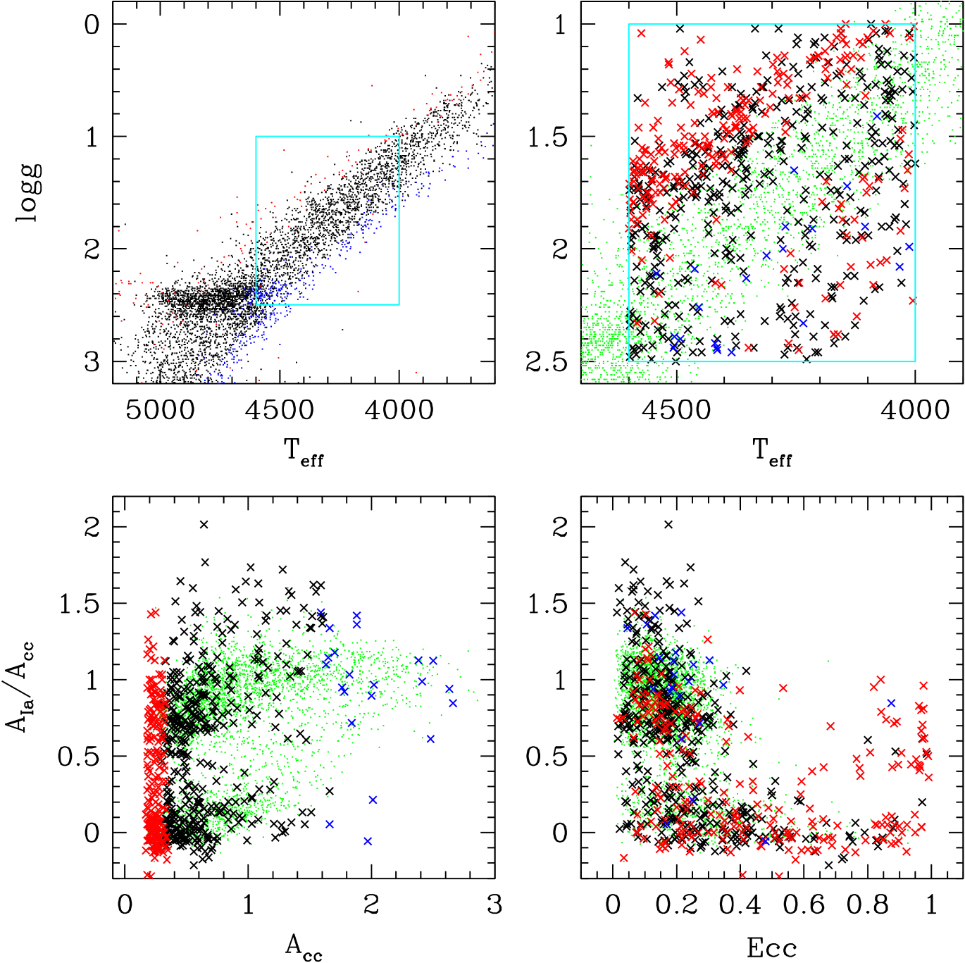
Figure 21 presents a more global view of the high- stars, selected as the sample members with modified values in the highest 2%, showing their distributions in vs. , vs. , and vs. orbital eccentricity (taken from the DR17 AstroNN catalog). The high- stars span the sample’s entire range in these parameters, but they do not follow the same distribution as the background stars (green dots, a random subset of our full sample). The high- stars are preferentially low metallicity, which is physically plausible because it is easier to perturb abundances (e.g., with mass transfer) if they are low to begin with, but which could also be a sign of measurement errors when features are weak. In the - diagram, most of the high- stars have low for their , which is an expected consequence of their preferentially low metallicity. However, the low metallicity stars that have high are likely to be cases where anomalous abundance patterns are affecting the spectroscopic estimates or where unusual properties of the spectrum (e.g., broad lines from high rotation) are producing erroneous values of and perhaps of the abundances as well. We find high- stars throughout the thin and thick disk populations, and they are clearly overrepresented among the high eccentricity, high-Ia population that likely corresponds to accreted halo stars. We return to this point in subsequent sections.
The literature on chemically peculiar stars is voluminous and rich. The examples in Figure 20 illustrate the possibilities for pursuing such studies with 2-process residual abundances. For our high-SNR disk star sample, the top 2% of the distribution already corresponds to nearly 700 stars, so exploiting this approach will be a substantial research effort in its own right. While there are many ways to find chemically anomalous stars, 2-process residuals have the virtue of automatically relating a star’s abundances to values that are typical for its metallicity and [/Fe]. This normalization makes it easier to identify stars that have moderate deviations across multiple elements but no single extreme values, such as the first example in Figure 20. Using machine learning techniques to pick out stars whose abundance patterns have low conditional probability given their values of and is another potentially powerful approach to this problem, well suited to take advantage of large homogeneous data sets like APOGEE (TW21).
7 Residual abundances of selected stellar populations
One goal of 2-process modeling is to assist the identification of chemically distinctive stellar populations, generically referred to as chemical tagging. Describing a star’s elemental abundance measurements with two parameters and residuals does not create new information, but it may improve the effectiveness of tagging algorithms by extracting two dimensions that vary widely in the disk, bulge, and halo populations and that shift many abundances in a strongly correlated, non-linear way. The 2-process+residual decomposition also prevents one from multi-counting abundance deviations that all reflect the same underlying changes in the bulk levels of a star’s CCSN and SNIa enrichment. We plan to pursue chemical tagging with residual abundances in future work. Here we illustrate prospects with the simpler but related exercise of examining residual abundances of selected stellar populations.
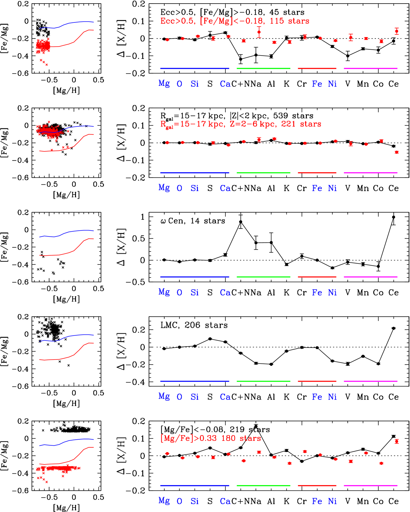
Figure 21, and Figure 25 below, suggest that the high eccentricity population may have distinctive abundances, particularly those high eccentricity stars that lie significantly above the plateau. This high-Ia (low-), high eccentricity population was identified by Nissen & Schuster (2010) as the likely remnant of a disrupted dwarf galaxy. Evidence for a dynamically distinct population became much stronger with Gaia data, and the accreted population is now identified as the remnant of the relatively massive “Gaia Sausage/Enceladus” (GSE) dwarf galaxy that merged early in the Milky Way’s history (Belokurov et al., 2018; Helmi et al., 2018). In the top right panel of Figure 22, black points show the median residual abundances of the 45 stars in our SN100 disk sample that have orbital eccentricity , , and . We estimate uncertainties in these medians as the dispersion of medians of 1000 bootstrap resamplings, i.e., for each resampling we choose 45 stars from the sample with replacement and compute the median, then take the standard deviation of these medians as the representative error bar. The median abundances of C+N, Na, Al, Ni, V, Mn, and Co are all depressed by 0.05-0.12 dex relative to other disk stars with matched values of . The median Ca abundance is elevated by a small but statistically significant 0.03 dex. By contrast, the median residual abundances for the high-eccentricity low-Ia stars () are statistically compatible with zero (red points). GSE stars are chemically distinct from other high-eccentricity stars in their ratios, and they are distinct from disk stars with similar metallicity and in their abundances of multiple odd- elements. The distinctive abundances of these stars may contribute to the drop of median [X/Mg] ratios in the lowest bin of the high-Ia population, seen in Figures 5-7 for C+N, Na, Al, Ni, Mn, and Co.
The second row shows stars with and satisfying our usual , , and cuts (§3) and . The 2-process model is “trained” using stars with , so none of the stars at contributed to calibrating the process vectors and . Nonetheless, the median residual abundances of all elements in this population are within 0.02 dex (and mostly within 0.01 dex) of zero. Despite their presence in the outer reaches of the stellar disk, these stars have APOGEE abundances very close to those of low metallicity, high-Ia stars in the rest of the disk. This similarity could indicate that these stars were born at smaller and migrated outward, or it could simply indicate that their enrichment history was similar despite their distinctive location. The outer disk is warped, with substantially more stars in the anti-center direction at these radii residing at large positive than at large negative . Red points show stars in the same radial range with . This population also has median abundances within 0.02 dex of the main disk population, except for Ce which is depressed by 0.05 dex. At larger (), Hayes et al. (2018) have found that stars in the “Triangulum-Andromeda” overdensity (Majewski et al., 2004; Rocha-Pinto et al., 2004; Sheffield et al., 2014) also have APOGEE abundance ratios similar to those of normal Milky Way disk stars.
One of the most dramatic abundance outliers in Figure 20 is a member of Cen, and we first noticed Cen as a distinctive population in our analysis because many of the extreme high- stars at low metallicity had similar sky coordinates. In the third row of Figure 22 we have selected all stars in the SN100 disk sample that have angular coordinates within of the cluster center at , and heliocentric velocity . The 14 stars selected have a mean with a dispersion of , while other sample stars that satisfy the angular selection have heliocentric velocities of to . The Cen stars have values ranging from our sample cutoff of up to . Like the star shown in Figure 20, their median residual abundances of C+N and Ce are extremely elevated (by 0.9-1 dex), and their median Na and Al residuals are +0.4 dex. Ca, K, Ni, and Co all show median deviations at the 0.1-0.2 dex level. Many of these stars have below the plateau value of , so they are assigned (unphysical) negative values of . The negative median deviations of most iron-peak elements may be a consequence of the 2-process predictions extrapolating poorly to this regime. Three of the Cen stars have near the median sequence of the low-Ia disk population. Like the other Cen members, these three stars all have extremely elevated (0.7-1.1 dex) C+N, Na, Al, and Ce, positive Ca residuals (0.1-0.2 dex) and negative Ni residuals (0.05-0.25 dex). Mészáros et al. (2021) present an APOGEE analysis of a much larger sample (982 stars) of Cen members, identifying multiple sub-populations in the (Fe,Al,Mg) distribution and examining abundance ratio trends in detail (see also Johnson & Pilachowski 2010).
In the fourth row we show residual abundances for stars identified as probable members of the LMC by Hasselquist et al. (2021), drawn from several different APOGEE programs targeting LMC stars (Nidever et al. 2020; Santana et al. 2021). For this sample we drop our geometrical cuts, but we do apply the same cuts in , , , and SNR to ensure a fair comparison to stars in our disk sample. We caution that of the 10655 LMC candidates in our original sample only 207 pass our and cuts. Most stars are lower because they must be luminous in order for APOGEE to obtain high SNR spectra at the distances of the LMC. It is possible that stars passing our cut are on the tail of the error distribution and have systematic abundance errors as a result.
Taking the measurements at face value, we note first that the 2-process model trained on Milky Way disk stars predicts the median LMC abundances of many APOGEE elements to 0.1 dex or better, which is an impressive degree of similarity given the radically different star formation environments and enrichment histories. However, several elements show median depressions of 0.15-0.2 dex (Na, Al, Ni, V, Co), and C+N and Mn show median depressions of 0.07 and 0.11 dex, respectively. The largest deviation is a 0.22-dex enhancement of Ce, and S and Ca show median enhancements of 0.10 and 0.06 dex. Similar deviations are found by Hasselquist et al. (2021) comparing the median [X/Mg] ratios of the LMC to values for the high-Ia Milky Way disk in the overlapping metallicity range. The tracks of the LMC imply a low star formation efficiency at early times, and an upward turn in at high suggests a substantial increase of star formation in the past (Nidever et al. 2020; Hasselquist et al. 2021), in qualitative agreement with photometric studies (Harris & Zaritsky, 2009; Weisz et al., 2013; Nidever et al., 2021). The different enrichment history of the LMC has left its imprint on the relative abundances of Ce, Ni, and multiple odd- elements in addition to the ratios.
Comparison of disk and LMC abundances can be improved by selecting a disk sample with the same distribution as the LMC sample, as for the disk-bulge comparison by Griffith et al. (2021a). This approach can also be applied to APOGEE observations of the Sgr dwarf and tidal stream (Hayes et al., 2020), and with lower metallicity samples it can be used to compare the Milky Way disk and halo to other dwarf satellites observed by APOGEE (Hasselquist et al. 2021) and to compare the satellites among themselves. Interpretation of these results would be aided by chemical evolution models that predict relative enrichment patterns for AGB elements and elements with metallicity-dependent yields in different regimes of star formation efficiency and star formation history.
All of the above populations are selected based on geometric and kinematic criteria. The final row of Figure 22 shows residual abundances for stars in our main disk sample selected to have unusually high or low values of [Mg/Fe], roughly of the sample in each case (see Figure 1 for reference). Red points show stars that lie at least 0.03 dex above our adopted plateau value of . The other elements that enter the 2-process fit (O, Si, Ca, Ni) have median deviations below 0.02 dex, so this population does not seem to arise from unusual values of Mg or Fe in isolation. The median residual [Mg/Fe] is 0.008, significantly smaller than the -dex offset from . The 2-process model assigns negative (unphysical) values of to these stars, and the -dex median residuals for many of the elements with large (0.08 dex for Ce) may be a consequence of extrapolating the model to this extreme regime. K shows an intriguing -dex median residual even though it has . A plausible scenario is that the enrichment of these rare high-[Mg/Fe] disk stars is dominated by CCSN that have moderately lower Fe and Ni yields relative to elements, perhaps just from stochastic sampling of the IMF. As previously noted, many Cen stars have high [Mg/Fe], but the high-[Mg/Fe] population as a whole does not show the extreme residual abundances of the Cen population. The AstroNN parameters for these stars indicate preferentially old ages and a wide range of eccentricities, as one would expect from their high [/Fe] ratios, but they exhibit no obvious clumping in and .
The stars with (black points) do show distinctive abundances, most notably for Na (0.17 dex) and Ce (0.11 dex). The small residuals for O, Si, Ca, and Ni again implies that this population is not produced by poor Mg or Fe measurements or by isolated variations of these two elements. These stars have a mean AstroNN age of only , as expected based on Figure 17 and their high values of . The elevated Na and Ce residuals of this population are thus another facet of the correlation of these residuals with age, seen previously in Figure 18. However, S and C+N residuals do not show strong correlations with age but nonetheless exhibit -dex enhancements in this low-[Mg/Fe] population. If we consider the far more numerous () stars with , the median residuals of Na and Ce are only 0.014 dex and 0.020 dex, respectively, and median residuals of all other elements are smaller than 0.01 dex. Thus, the very low [Mg/Fe] stars do appear to be a distinct population, in both age and abundance patterns. These stars are preferentially low eccentricity and close to the Galactic plane, as expected for a young population, but they also do not exhibit obvious clumping in and .
8 Beyond two processes
The covariance of residuals demonstrated in Figure 15 (and by TW21) implies that we should do more than simply look at residuals element-by-element. Theoretically, we would like to describe stellar abundances in terms of all of the astrophysical processes that contribute significantly to their origin. Empirically, we can describe star-by-star variations in terms of components that vary multiple elements in concert. The latter approach is similar in spirit to applying principal component analysis to stellar abundances (Andrews et al., 2012; Ting et al., 2012; Andrews et al., 2017), but focusing on residuals allows us to first remove the CCSN and SNIa processes that we know make dominant contributions to most APOGEE elements. Both approaches are connected to the underlying question of the dimensionality of the stellar distribution in chemical abundance space: if we have measurements of abundances for every star, how well can the full distribution (not just the mean trends) of those abundances in -dimensional space be approximated by a 1-dimensional curve, a 2-dimensional surface, a 3-dimensional hypersurface, etc.? (For related discussion see §5.1 of TW21.) In this section we first discuss the generalization of the 2-process model to additional processes (§8.1) and the relation between process fluctuations and residual correlations (§8.2). We then turn to an empirical approach of fitting correlated residual components (§8.3) and look for correlations of those components with age and kinematics (§8.4).
8.1 An N-process model of abundances
As a mathematical exercise, it is trivial to generalize the 2-process model of §2 to processes. The abundance of element in a star is given by
| (33) |
We use greek subscripts to denote processes and latin subscripts to denote elements, and for compactness we have omitted the -dependence of and have not introduced a separate index to denote the star. As with the 2-process model, the process vectors are taken to be universal at a given metallicity across all stars in the population, while the amplitudes vary from star-to-star and are defined to be for a star with solar abundances. The generalizations of equations (19,20,6,8) are:
| (34) | |||||
| (35) | |||||
| (36) | |||||
| (37) |
where all sums are over .
In our discussion below we will take to represent CCSN and to represent SNIa. The obvious choice for is AGB enrichment, while larger could represent rarer processes that are important for some elements, such as neutron star mergers, magnetar winds, etc. However, we caution that partitioning enrichment channels into a moderate number of discrete processes is an approximate exercise, and a characterization that is adequate for one stellar abundance sample may become inadequate for a sample with higher measurement precision or a different range of stellar populations. For example, at one level of precision it may be fine to treat CCSN enrichment as a single IMF-averaged process, while at higher precision or for a metal-poor stellar population one may need to consider stochastic variations in IMF sampling. The mass dependence of AGB yields is different for different elements, and because the lifetimes of stars depend strongly on mass it may not be adequate to describe AGB enrichment in terms of a single IMF-averaged process. For any source (CCSN, SNIa, AGB, etc.), the relative production of elements that have very different metallicity dependence will change to some degree with the enrichment history of the stellar population.
Despite these caveats, an N-process description offers a powerful way to isolate two largely distinct aspects of Galactic chemical evolution (GCE) models: nucleosynthetic yields and enrichment history. While the enrichment history — which is itself affected by accretion, star formation, and gas flows — can strongly affect metallicity distribution functions, it has much more restricted impact on element ratios. In the N-process language, the enrichment history determines the joint distribution of process amplitudes and its trends with age and kinematics, but the nucleosynthetic yields determine the process vectors with little dependence on enrichment history. For 2-process modeling with APOGEE data, we have the advantage that some elements (O, Mg) are expected to arise almost entirely from CCSN and that Fe and Ni provide well measured diagnostics of SNIa enrichment. To characterize a third process, we would like one or more well measured elements that have minimal contributions from SNIa to serve as markers of this process. There are no ideal candidates in current APOGEE data, though Ce is a possibility, and if C and N could be individually corrected to birth abundance values then they might provide a further foothold for quantifying AGB enrichment. With GALAH data or joint APOGEE-GALAH data sets (Nandakumar et al., 2020), neutron capture elements such as Ba, Y, and Eu may provide valuable diagnostics of additional processes.
8.2 Process fluctuations and residual correlations
The N-process model provides a conceptual language for thinking about residual abundance correlations like those shown in Figs. 15 and 16. First, we adjust equation (33) to allow “intrinsic noise” in individual abundances that is not described by the N-process model,
| (38) |
where would be the fractional variance of the residual abundance of element if we knew each star’s exactly, and we assume and for . If the model includes all processes that are important for the production of element then we expect . The 2-process fit is applied to elements that we expect to be dominated by , 2 (CCSN and SNIa). At given values of , , the stellar population has mean values of the process amplitudes for . The mean abundances in the population are
| (39) |
To predict the correlations of observed abundance residuals, we must allow for the fact that we do not know each star’s true values of and but instead have estimates of these quantities, which we denote by and . Our abundance measurements are also affected by observational noise
| (40) |
where is the fractional variance of the measurement errors. The residual abundances for a given star are
| (41) |
To approximate these residuals we introduce
| (42) |
and
| (43) |
using to represent observational and intrinsic differences, respectively. We make the first-order Taylor expansion
| (44) |
Writing
| (45) |
and
| (46) |
and applying equations (42-46) to equation (41) yields, after some manipulation,
| (47) | |||||
The first term represents the sum of “intrinsic noise” and observational noise. The second term is the most physically interesting, showing the impact of random fluctuations in additional processes beyond CCSN and SNIa. The last four terms represent the “measurement aberration” discussed by TW21 and in §5.4 above.
To obtain an expression for covariance that is tractable enough to be conceptually useful, we ignore the last two terms of equation (47), and we assume that , that , and that for . It is not clear that any of these approximations is accurate in a realistic case, but the resulting expression does illuminate several of the effects that influence the covariance of residuals:
| (48) | |||||
If measurement aberration is small enough to be neglected, then off-diagonal covariances all arise from the second term. These off-diagonal covariances can be small either because the variation in process amplitudes at fixed is small, so that , or because the processes make small contributions to the abundances of elements or , so that . Covariances alone offer no way to distinguish these two cases. However, if the second term dominates over the other three, then the off-diagonal correlation will be large for elements that come largely from a single process, even if the covariance is small because .
As a concrete example of this point, consider a pair of elements whose production is dominated by AGB stars. Because AGB enrichment is delayed in time like SNIa, we expect to increase with both and , and at solar abundances we expect . Even if the variance of is small, it is responsible for most of the variation in the two elements, so the correlation coefficient will be near unity even though itself is small. In fact the correlation coefficient can be large even if the elements themselves have large contributions from CCSN and SNIa, because the variation at fixed still comes from other processes. However, in this case it is more challenging to distinguish the true correlations caused by additional processes from the artificial correlations induced by measurement aberration (non-zero and ).
In light of this discussion, the large correlation coefficients seen in Figure 16 or in Figure 8 of TW21 are not surprising. Even when element abundances are predicted to high accuracy by a 2-parameter model, or by conditioning on two elements, the intrinsic correlations of the residual abundances will be high if they are dominated by a small number of additional processes.
An interesting feature of equation (48) is that it generates only positive correlations if the are positive. Anti-correlations can arise if the process amplitudes themselves are anti-correlated, , a possibility that (for simplicity) we did not allow in deriving equation (48). They could also arise from processes that deplete some elements (negative ) but produce others, which could happen in unusual circumstances. Measurement aberration may easily lead to , since one is fitting parameters to abundances that have contributions from both processes. The largest anti-correlations in Figure 16 involve elements that contribute to the fit, and similar features appear in the simulated data, which suggests that these anti-correlations are dominated by measurement aberration. If intrinsic anti-correlations can be well established empirically then they could be quite physically informative, since they are not easy to produce.
8.3 Fitting additional components
While we would ideally like to infer values of for additional processes from the 2-process residuals, then fit to obtain values of for individual stars as we did for and , it is not clear that there is any practical way to do this without theoretical priors on what elements to assign to what processes. For the current APOGEE data, the challenge is exacerbated by the fact that the residuals from the 2-process predictions are usually not much larger than the estimated observational noise, and the observational error distribution is itself uncertain. Correlation of residuals can be measured at high significance in a large sample, but the residual abundances of individual stars are mostly measured at low or moderate significance. In future work, we will use chemical evolution simulations that incorporate multiple enrichment channels and stochastic variations to guide strategies for isolating additional processes from observed abundance distributions.
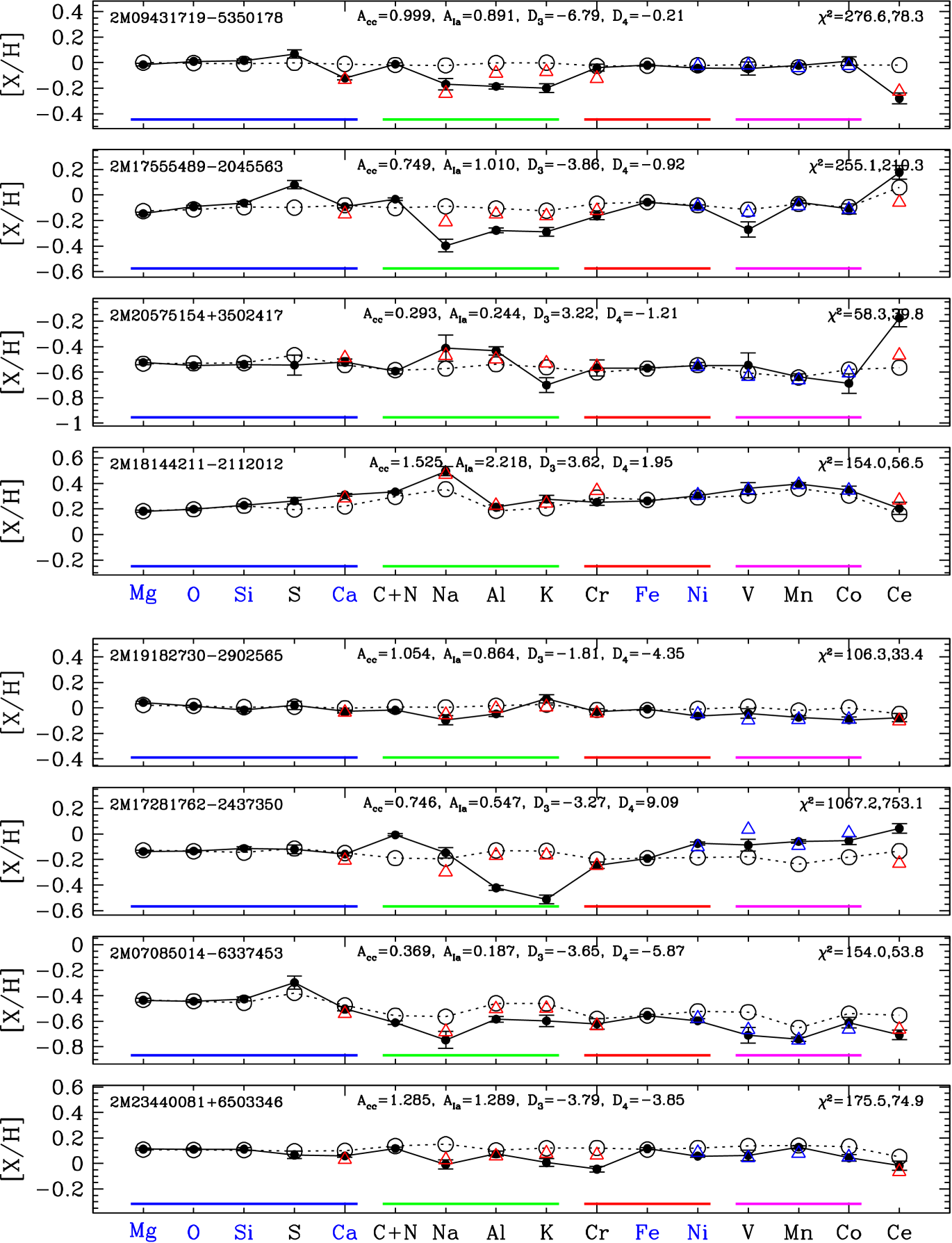
For a data-driven approach, the most obvious tack is to apply principal component analysis (PCA) to our estimate of the intrinsic covariance matrix of residual abundances in Figure 15d. The new components would be the eigenvectors of this matrix that have the largest eigenvalues and thus explain the largest fraction of the variance. However, there is no reason to expect the physical enrichment processes to produce orthogonal components in abundance space, so even if the intrinsic covariance matrix were perfectly known the eigenvectors would represent mixtures of the physical processes. We have also found that the results of PCA are sensitive to minor details of how we treat the data and measure the covariance, making physical interpretation difficult. For now we adopt a simpler approach that is loosely motivated by the discussion in §8.2.
We pick a subset of elements that show significant correlations and that we suspect on physical grounds should be treated as a group. For each group, we have a covariance matrix of residual abundances . Suppose that the residuals within this element group arise from a single process plus uncorrelated “noise” that may include both observational noise and intrinsic element-by-element scatter:
| (49) |
In contrast to our notation in §8.2, , , and are all in dex, and we use in place of because it represents a deviation from the mean amplitude rather than an amplitude that is defined to be unity at solar abundances.
Under these assumptions, the predicted covariance matrix of these elements is
| (50) |
where represents the variance in the residual abundance that is not explained by the correlated deviations. As previously noted, from covariances alone we cannot distinguish between large with small and small with large . We arbitrarily take and infer the corresponding values of by minimizing the cost function
| (51) |
i.e., by minimizing the squared deviation between the predicted and observed off-diagonal values of the covariance matrix for the elements in the group. The values of then follow from matching the predicted and observed diagonal components (equation 50). We require to have sufficient off-diagonal constraints to determine the values of . Since we have assumed , we see from equation (49) that if then the typical residual abundances of can be explained predominantly by the correlated fluctuations with other elements in the group, while if then independent fluctuations dominate over this correlated contribution. The relative values of indicate the relative deviations of elements associated with process fluctuations .
Based on Figure 16a we have selected two element groups, one () comprised of Ca, Na, Al, K, Cr, and Ce, and the second () comprised of Ni, V, Mn, and Co. There is some arbitrariness in this choice. For example, Na and K show significant correlations with the iron-peak group in addition to Ca, Al, and Ce, and Al is (weakly) anti-correlated with Ce and (weakly) positively correlated with Ni, V, and Co. One must be cautious about naively applying nucleosynthesis intuition to residual abundances because we have already removed the main effects of CCSN and SNIa through the 2-process fit. For example, even though K comes mainly from CCSN and Mn comes mainly from SNIa, the deviations from typical K and Mn abundances at a given and could be physically linked.
Conceptually, we could imagine that Ca, Na, Al, K, Cr, and Ce all have contributions from AGB stars, and that positive and negative values of represent stars that have more or less than the average amount of AGB enrichment relative to stars with the same and (2nd term on the r.h.s. of equation 47). The component could be driven by a subset of SNIa (or even CCSN) that have higher yields of Ni, V, Mn, and Co, and positive and negative values of would represent stars enriched by more or fewer than the average number of such unusual supernovae. However, this physical interpretation is by no means unique. These caveats notwithstanding, our approach offers a plausible way to combine physical expectations with data-driven lessons to search for correlated element deviations on a star-by-star basis.
| Elem | ||||
|---|---|---|---|---|
| Ca | ||||
| Na | ||||
| Al | ||||
| K | ||||
| Cr | ||||
| Ce |
Note. — Coefficients for the elements comprising component 3. For a star with amplitude deviation the model prediction of changes by dex (equation 49). The variance not explained by the correlated contribution is (equation 50). When fitting values for individual stars, elements are weighted by the inverse-square of (equation 52).
| Elem | ||||
|---|---|---|---|---|
| Ni | ||||
| V | ||||
| Mn | ||||
| Co |
Note. — Coefficients for the elements comprising component 4.
Tables 2 and 3 report our inferred values of and for these two components. The sum of and is equal to the variance of the element’s residual deviations from the 2-process fit (equation 50). For a star with a given value of , the change in the predicted from adding component is (equation 49). We estimate the value of for each star from the weighted average
| (52) |
which minimizes . We weight by the inverse of the variance estimated from the 16-84% percentile range of the observed residual abundance distribution, which is less sensitive to outliers than the variance itself; we list the values of in the fourth column of Tables 2 and 3. This choice weights the elements more uniformly than if we used the observational error estimates. We omit elements that have flagged data values for a given star. The final column of the tables gives the relative change of the elements associated with each component. A given value of changes the predicted Ce and Na abundances by about twice as much as the predicted Ca and K abundances and by -5 times as much as the predicted Cr and Al abundances. The range of values is somewhat smaller, with V the element most sensitive to and Ni the least sensitive. With the exception of Ca, the values of exceed those of , indicating that the correlated deviations associated with these two processes explain only a small portion of the observed residual abundance variance for these elements. This finding is consistent with the results of TW21, who concluded that at least five “components” (implemented there as individual conditioning elements) beyond Mg and Fe are needed to reduce residual fluctuations in APOGEE abundances to a level consistent with observational uncertainties alone.
Figure 23 shows examples of fits to eight stars that have unusually large values (in the outer 2% tails) of or or both. In each of these cases, the large or reduces coherent residuals across most or all of the elements in the component, typically 0.05 dex or larger. However, there are also examples (not shown) where a single highly discrepant abundance drives a large component amplitude. Not surprisingly, for these stars selected to have large or the 4-process fit achieves a large reduction relative to the 2-process fit, but the median reduction across the whole sample is only 4.8. The first star shown in Figure 23 is also the first star shown in the selection of high- stars in Figure 20. The addition of and (unimportant in this case) reduces from 277 to 78, though it still does not produce agreement within the reported observational uncertainties for all of the deviant elements. This pattern, a substantial reduction but significant remaining deviations after the 4-process fit, holds for most of the examples, though the component typically explains the deviations (usually smaller) in Ni, V, Mn, and Co fairly well. The final two stars in Figure 23 have unusually large negative values of both and .
8.4 Correlations with age and kinematics
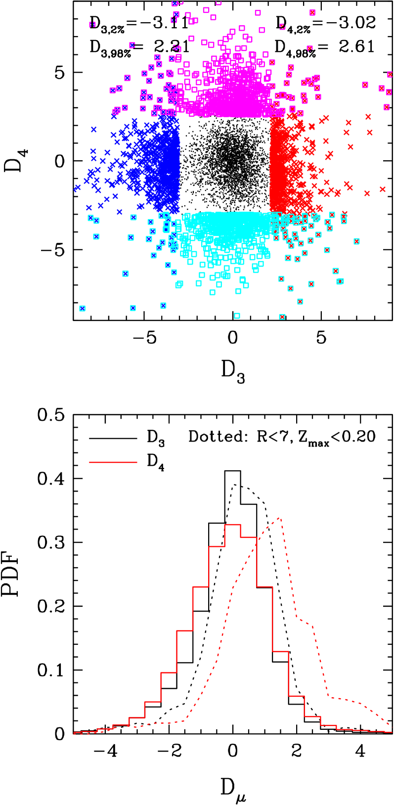
In the top panel of Figure 24, colored points show for stars in the outer 2% tails of the or distributions, and black dots show a random sampling of stars in the inner 96% of both distributions. The values of and are essentially uncorrelated, with a Pearson correlation coefficient of , changing to if we restrict to the inner 96%. The lower panel plots the distribution of component amplitudes, which are slightly skew-negative for both and . For the most part, we find no obvious trends of or with Galactic position. However, stars near the midplane in the inner Galaxy (, ) tend to have slightly higher values of and , as shown by the shifted distributions in this panel. In other words, stars of the inner thin disk tend to have slightly elevated values of the ten elements that contribute to these components, relative to other stars with the same values of and . The mean values of and for this population are higher by 0.44 and 1.31, corresponding to mean differences and of only 0.013 dex and 0.031 dex for the two most sensitive elements (Ce and V, respectively), and smaller shifts for other elements. This subtle change of chemistry is detectable because we have many stars to average over and have controlled through 2-process fitting for the much larger differences between the inner thin disk and the full sample in and (mean offsets of 0.56 and 0.42, respectively, corresponding to shifts of dex in and dex in ). If we define the inner thin disk based on the current midplane distance rather than dynamically estimated maximum distance, i.e., by instead of , then the shift of the distribution is similar but the shift of the distribution is weaker, with a mean offset of only 0.25 instead of 0.44.
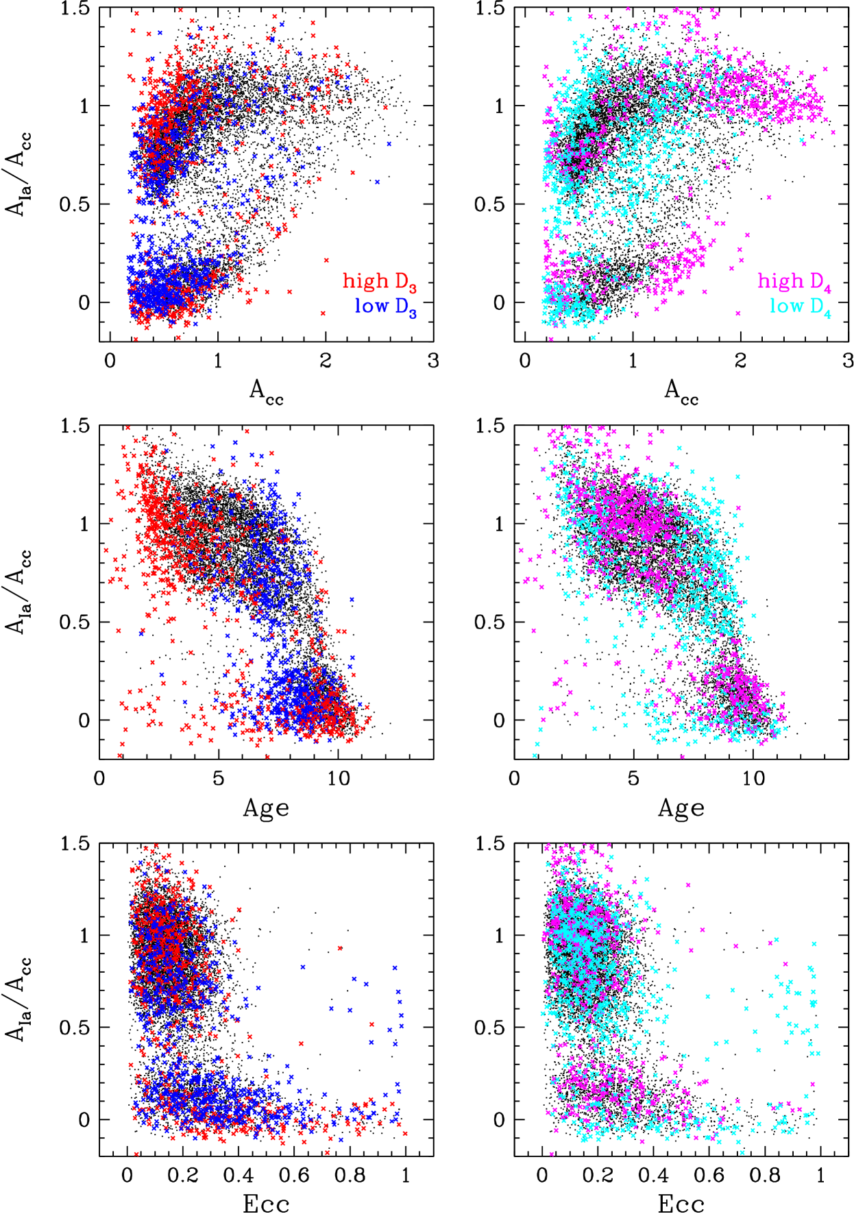
Figure 25 plots the outliers (left) and the outliers (right) in the planes of vs. , vs. age, and vs. eccentricity, with a random subset of the full sample plotted for comparison. The outliers arise throughout the distribution with no obvious clustering, though there is some overrepresentation of low- outliers among metal-rich stars that are in between the low-Ia and high-Ia populations (, ). The outliers are present at all ages, though there is a clear tendency for high- stars to have younger ages (by ) in the high-Ia population, and a significant number of high- stars have low and young estimated ages. There is also a concentration of low- stars at ages of 6-8 Gyr.
Outliers are also widely distributed in the plane of vs. eccentricity. However, there is a clear excess of stars with low and low that have high eccentricity and elevated values of relative to other high eccentricity disk stars. This population also has low values of (and thus of ), near the lower boundary of our sample. The second-to-last star in Figure 23 is a member of this high-eccentricity population, with , though it was chosen for this plot based on its and values alone. We have already seen this population stand out in the sample of high- stars (Figure 21), and the top row of Figure 22 shows that the “accreted halo” stars (a.k.a. GSE stars) have negative residuals of all four elements in the component and of two of the elements (Na and Al) in the component. The extreme and values are another signature of the distinctive abundance patterns of this population.
We view this analysis as a first step in exploiting the information encoded by correlated patterns of residual abundances. The component formalism introduced here offers a data-motivated way to compute average deviations of correlated elements with appropriate relative weights, obtaining measurements that are higher SNR than the deviations of individual elements. The geometric, age, and kinematic patterns in Figures 24 and 25 demonstrate that the and component amplitudes are capturing genuine physical distinctions among stellar populations. However, extreme values of these components arise in stars throughout the disk with a wide range of ages, kinematics, and CCSN and SNIa enrichment levels.
9 Conclusions
We have developed a novel approach to statistical analysis of multi-element abundance distributions of large stellar samples and applied it to the final (DR17) data release of APOGEE-2 (from SDSS-IV), which includes a homogeneous re-analysis of spectra from APOGEE in SDSS-III. Our primary sample consists of 34,410 stars with , , , , and , with the last two cuts adopted to limit the impact of differential systematics on abundance measurements. We consider the -elements Mg, O, Si, S, and Ca, the light odd- elements Na, Al, and K, the even- iron-peak elements Cr, Fe, and Ni, the odd- iron-peak elements V, Mn, and Co, the s-process element Ce, and the element combination C+N, employed because C+N is conserved during dredge-up processes that change the individual C and N surface abundances in the convection zones of red giants. Following W19 and Griffith et al. (2019), we fit the median trends of low-Ia and high-Ia populations with a 2-process model that approximates stellar abundance patterns as the sum of a CCSN contribution that tracks Mg enrichment and an SNIa contribution that tracks the SNIa Fe enrichment. For elements with substantial contributions from processes other than CCSN and SNIa, the 2-process model approximately separates a “prompt” and “delayed” enrichment component. With the global model parameters ( and for each element X in 0.1-dex bins of ) determined from the median sequences, we proceed to fit each sample star’s measured abundances with two free parameters ( and ) that scale the amplitude of the two processes (equation 1; Figure 3). We characterize each star by its values of and and the residuals from this 2-process fit.
9.1 Median sequences and their implications
For the 14 elements in common with W19’s analysis (based on DR14), we find similar results for median sequences and thus draw similar conclusions about the relative CCSN and SNIa contributions. Among the -elements, Si and Ca are inferred to have significant SNIa contributions, though not as large as those of iron-peak elements. Among the light odd- elements, Al and K appear to be dominated by CCSN, but the low-Ia and high-Ia populations have substantially different [Na/Mg] ratios, implying a large delayed contribution to Na that could be associated with SNIa or AGB sources. Among the iron-peak elements, Mn is inferred to have the largest SNIa contribution. The most significant differences from DR14 are that the increasing metallicity trend of [Al/Mg] becomes flat in DR17 and that the steeply rising trends of [V/Mg] with metallicity become shallower. While W19 fit the median trends with power-law metallicity dependence for the CCSN and SNIa processes, here we adopt a generalized metallicity dependence in bins of [Mg/H] such that the 2-process model reproduces the observed [X/Mg] sequences exactly. Several elements — Na, V, Mn, Co, and to a lesser extent Ni — show evidence of rapidy rising SNIa yields for , though this conclusion is sensitive to the accuracy of APOGEE’s abundances in the super-solar metallicity regime.
For [(C+N)/Mg] and [Ce/Mg], both new to this study, we find substantial gaps between the median sequences of low-Ia and high-Ia stars, implying a substantial contribution from delayed sources. For these elements, the delayed source is probably AGB enrichment rather than SNIa. The metallicity dependence of the high-Ia [Ce/Mg] sequence is non-monotonic, peaking at , similar to the behavior seen in GALAH DR2 for the neutron-capture elements Y, Ba, and La (Griffith et al., 2019). The rising trend at low [Mg/H] can be understood from the increase of seed nuclei for neutron capture, which shifts to a falling trend when the ratio of seed nuclei to free neutrons becomes too large to allow the s-process to reach heavy nuclei (Gallino et al., 1998). The low-Ia/high-Ia median trends for [(C+N)/Mg] and [Ce/Mg] are a powerful empirical test for supernova and AGB yield predictions. The and values that we derive for other elements allow tests of supernova yield models (e.g., Griffith et al. 2021b) that are insensitive to uncertainties in other aspects of disk chemical evolution.
9.2 Residual abundance scatter and correlations
Turning to residual abundances, we find that the distribution of residuals from the 2-process predictions is narrower than the distribution of residuals from the observed median sequences for all of the elements that APOGEE measures well (i.e., with mean observational uncertainties below 0.03 dex; see Figure 12). This reduction implies that much of the observed scatter in [Mg/Fe] at fixed [Mg/H] within the low-Ia and high-Ia populations is intrinsic (Bertran de Lis et al., 2016; Vincenzo et al., 2021a), reflecting real variations in SNIa/CCSN enrichment ratios, and that accounting for these variations correctly predicts variations in other elements. Similarly, we find that using residuals from the 2-process predictions rather than residuals from median sequences largely removes trends with stellar age and orbital parameters (Figures 18 and 19). However, Ce and Na residuals both show clear correlations with age in the high-Ia population, with the youngest stars showing higher abundances of both elements relative to other stars with similar and .
After subtracting the observational uncertainties reported by ASPCAP from the observed scatter, we infer rms intrinsic scatter in the 2-process residuals ranging from dex to dex for most elements, with values up to dex for Na, K, V, and Ce (Figure 13). Our estimates of the characteristic intrinsic scatter and of the relative scatter among different elements agree quite well with the estimates of TW21 for scatter in abundances conditioned on [Fe/H] and [Mg/Fe], and with those of Ness et al. (2019) for scatter conditioned on [Fe/H] and age.
More informative than the element-by-element scatter is the covariance of residual abundances between elements (equation 31). We find significant off-diagonal covariances among many elements, with many values clearly exceeding the expected covariance from observational errors alone (Figure 15). Our estimates of 2-process residual correlations (Figure 16) agree qualitatively with those found by TW21 for conditional abundance residuals despite many differences in methodology, a reassuring indication of the robustness of the results. Correcting the observed covariances for observational contributions remains uncertain because the observational error distributions are not fully understood. The clearest findings are two “blocks” of correlated residuals, one involving Ca, Na, Al, K, Cr, and Ce and the other comprised of Ni, V, Mn, and Co. For most correlated element pairs, the bi-variate distribution of residuals shows a consistent slope between the core of the distribution and the tails (see Figure 10 for examples). This structure suggests that the residuals are mostly driven by a continuous spectrum of variations, e.g., by the relative contribution of processes beyond CCSN and SNIa, or by stochastic sampling of the CCSN and SNIa populations combined with imperfect mixing in the ISM. The one striking exception to this rule is the (C+N)-Ce correlation (Figure 14), where the core of the distribution shows a clear anti-correlation but a population of rare outliers exhibits strong positive deviations of both (C+N) and Ce. These highly enhanced stars could be a consequence of mass transfer from AGB companions or of second-generation AGB enrichment in star clusters.
9.3 High- stars and selected populations
By automatically normalizing a star’s abundances to those of other stars with similar [Mg/H] and [Mg/Fe], 2-process fitting makes it easy to identify outlier stars with unusual measured abundance patterns. This approach is especially valuable for cases with moderate deviations (e.g., 0.05-0.1 dex) across multiple elements, which might be difficult to pick out in an eyeball scan of [X/Fe]-[Fe/H] diagrams. Unfortunately, easy identification does not mean easy interpretation, and a key challenge is distinguishing physical outliers from cases where measurement errors are much larger than the reported observational uncertainties. Among the physical outliers, some may be extreme examples of the same variations that produce residual correlations in the bulk of the population, while others may arise from rare physical processes that affect only a small fraction of stars.
Figure 20 presents a selection of eight stars from the that comprise the top 2% of the residual distribution. These examples include two stars with depressed Na, Al, and K abundances and low or high Ce, a carbon star that also has high measured abundances of Na, Al, and V, a “barium” star first identified by Smith & Suntzeff (1987) that is one of the extreme (C+N)-Ce outliers, a member of the Cen globular cluster with 0.5-1 dex enhancements in C+N, Na, Al, and Ce, and a N-rich star with elevated Al, Ce, and Si, which has been independently identified both as a possible globular cluster escapee (Schiavon et al., 2017; Fernández-Trincado et al., 2017; Fernández-Trincado et al., 2019a, 2020c, 2020b) and as a member of a small population of chemically peculiar stars with extreme P enhancement (Masseron et al., 2020a, b). Another star shows strong deficiencies of K and V, an effect that we see in multiple stars but that may be a consequence of radial velocity placing stellar features over strong telluric lines that are difficult to subtract precisely. Another shows a distinctive pattern of enhanced Na, elevated C+N and Mn, and depressed Al, K, and Cr. We also see this pattern in multiple outlier stars, but we remain unsure whether it represents an unusual physical abundance pattern or a subtle observational systematic.
Residual abundances may prove to be a powerful tool for chemical tagging studies, i.e., for identifying groups of stars that share distinctive abundance patterns suggesting a common birth environment. In this paper we have illustrated these prospects with the much simpler exercise of computing the median residual abundances of a few select stellar populations (Figure 22). Stars with high eccentricity, low metallicity (), and relatively low () have been previously identified as “accreted halo” stars (Nissen & Schuster, 2010), probably formed in the “Gaia-Sausage/Enceladus” dwarf (Belokurov et al., 2018; Helmi et al., 2018). Relative to 2-process model predictions, these stars have C+N, Na, and Al abundances that are low by about 0.1 dex and Ni, V, Mn, and Co abundances that are low by -0.1 dex. However, high eccentricity stars in the same range with have median abundance residuals consistent with zero. Stars observed by APOGEE in the LMC that overlap our disk star metallicity, , and range show a similar abundance pattern to the GSE stars, and a 0.2-dex enhancement of Ce. The 14 Cen members that fall in our disk sample show extreme (-dex) enhancements of C+N and Ce and large (-dex) enhancements of Na and Al. Stars in the outer disk (), either near the midplane () or well above it () have abundances entirely consistent with those of our sample, with the slight exception of a 0.05-dex median depression of Ce in the high- population. Each of these results is a target for chemical evolution models of these populations, and many other populations can be studied in similar fashion.
9.4 Beyond 2-process
We do not expect the 2-process model to provide a complete description of stellar abundances, and the intrinsic scatter of , the element-to-element correlations among residuals, the outlier stars, and the distinctive patterns of selected populations all demonstrate empirically that it does not. In §8 we have taken some first steps towards a more general “N-process” model. On the theoretical side, we have proposed a natural generalization of the 2-process formalism that can encompass an arbitrary number of additional processes, and we have shown, approximately, how variations in the relative amplitudes of those processes would translate into correlated residuals from the 2-process fits (equations 45-48). On the observational side, we have used the observed covariance matrix of residual abundances (Figure 15) to define two new “components” with weighted contributions of Ca, Na, Al, K, Cr, Ce (component 3) and Ni, V, Mn, Co (component 4). We then fit amplitudes and defining the deviations of these components to all stars, with by construction. We find stars with high and low values of and throughout the disk and widely spread in , , age, and kinematics (Figure 25). However, the GSE population has low and , the high- stars have preferentially young ages in both the low-Ia and high-Ia populations, and the coldest subset of the inner thin disk (, ) has slightly elevated mean values of and .
9.5 Prospects and challenges
The combination of 2-process fitting and residual abundance analysis is a potentially powerful new tool for interpreting multi-element abundance measurements in large spectroscopic surveys such as APOGEE, GALAH, and SDSS-V.555This approach may also prove valuable for lower resolution surveys such as LAMOST and DESI, but its natural application is to data sets that achieve precision of 0.01-0.05 dex or better for multiple elements that probe a variety of nucleosynthetic pathways. This method has much in common with the conditional PDF method of TW21, in which one matches stars in [Fe/H], [Mg/Fe], and other abundances or parameters as desired. Each method may have practical advantages for some applications. The greatest challenge to exploiting these approaches is fully characterizing the observational contributions to abundance residuals, to their correlations and systematic trends, and to abundance outliers. One way forward is to make more comprehensive use of repeat observations (see §5.4 of Jönsson et al. 2020) to map out the distribution and correlations of “statistical” errors, which arise from photon noise but also from effects such as telluric line contamination and varying line spread functions that are difficult to predict from models and simulations. A second is to exhaustively follow up a large sample of 2-process outliers and run to ground any observational systematics that give rise to them. A third is to compare results from different abundance analysis pipelines to determine which residual abundance correlations and outlier populations are robust and which are sensitive to analysis choices. Samples of stars with observations and abundance measurements from two separate surveys, such as APOGEE and GALAH, allow a complete end-to-end comparison for elements in common, as well as extending the number of elements that trace different astrophysical sources. For some investigations, high-resolution, high-SNR observations of smaller samples that are matched in stellar parameters, such as “solar twin” studies (Ram´ırez et al., 2009; Nissen, 2015; Bedell et al., 2018), may be a valuable complement to the larger samples from massive surveys.
Residual abundance analysis imposes stiff demands on the accuracy of stellar abundance pipelines. Even after restricting our sample to and , we find trends of residuals with that we must remove before measuring element-to-element correlations (Figure 10). To compare distinct populations such as bulge and disk or disk and satellites, one must create comparison samples that are matched in (e.g., Griffith et al. 2021a; Hasselquist et al. 2021) and/or condition on and as variables in addition to abundances (TW21). Such comparisons would become more straightforward if the systematics in APOGEE abundances were removed either by empirical calibration or, preferably, by identifying and correcting the effects that give rise to them.
There are numerous natural follow-ons to this initial effort in residual abundance cartography, some that can be done with the existing sample, some requiring similar analysis of different APOGEE subsets, and some involving new or different observational data. Systematic examination of the high- population should turn up a variety of physically unusual stars, perhaps including previously unknown categories. Comparison of samples with and without binarity signatures in their radial velocity variations could reveal more subtle impacts than the C+N/Ce outliers already identified. Residual abundances offer new ground for clustering searches in the high-dimensional space of chemistry and kinematics, especially useful for uncovering populations that could span a range of and . With the 2-process model “trained” on samples with matched and ranges, one can compare residual abundance patterns among the disk, bulge, halo, dwarf satellites, and star clusters, building on the results of Griffith et al. (2021a) and Hasselquist et al. (2021) and the examples in Figure 22. A third generation of the APOKASC catalog (Pinsonneault et al. 2014, 2018; Pinsonneault et al. in prep.) will soon provide asteroseismic masses, ages, and evolutionary states for APOGEE stars in DR17. This sample can be used to look for more subtle trends of residual abundances with age, to look for trends with evolutionary state or internal rotation that could be signatures of non-standard mixing processes, and to disentangle C+N into separate C and N components (see Vincenzo et al. 2021b). Combinations of APOGEE and GALAH data will provide cross-checks on common elements and a wider range of elements tracing a greater variety of nucleosynthetic origins. In combination with Gaia space velocities, residual abundances should be well suited to the program of Orbital Torus Imaging (Price-Whelan et al., 2021), which exploits the fact that stellar abundance patterns in steady state may depend on orbital actions but should be invariant with respect to their conjugate angles. The Milky Way Mapper program of SDSS-V will obtain APOGEE spectra for an order of magnitude more stars than DR17, enabling much more comprehensive mapping of disk, bulge, and halo abundance patterns and much more powerful constraints on clustering in chemo-dynamical space.
Theoretically, this approach would benefit from a new generation of Galactic chemical evolution models that predict joint distributions of multiple elements from multiple astrophysical sources. Models that combine stellar radial migration with radially dependent gas accretion, star formation, and outflow histories have achieved impressive (but not complete) success in reproducing many aspects of the observed joint distributions of metallicity, , age, , and (e.g., Schönrich & Binney 2009; Minchev et al. 2013, 2014, 2017; Johnson et al. 2021). A natural next step is to extend these models to additional elements, using yields that are theoretically motivated but also empirically constrained to reproduce observed median trends. Radial mixing of populations with different enrichment histories will then produce fluctuations in abundances at fixed and (or and ). These “mixture” models will provide useful guidance for extending the 2-process formalism, sharpening the ideas outlined in §8.
We suspect that stellar migration alone will prove insufficient to explain the observed level of residual fluctuations and their correlations. Radial gas flows and galactic fountains may also be important ingredients in chemical evolution (e.g., Bilitewski & Schönrich 2012; Pezzulli & Fraternali 2016), but we again suspect that they will alter mean trends without adding scatter in residual abundances. Instead we expect that explaining the observed residual covariances will require models that incorporate localized star formation and gradual ISM mixing, and it may also require stochastic sampling of the supernova and AGB populations. Recent galactic evolution models offer steps in this direction (Armillotta et al., 2018; Krumholz & Ting, 2018; Kamdar et al., 2019). Our results provide a quantitative testing ground for such models.
Over a decade of observations and increasingly sophisticated data analysis, APOGEE has obtained an unprecedented trove of high-precision, high-dimensional stellar abundance data, probing all components of the Milky Way and several of its closest neighbors. The combination of 2-process modeling and residual abundance analysis is one way to exploit the rich complexity of this data set, taking advantage of its high dimensionality and helping to disentangle the intertwined impacts of nucleosynthetic yields and Galactic enrichment history. Systematic application of these tools to APOGEE and its brethren, and comparison to a range of theoretical models, will teach us much about the physics of nucleosynthesis in stars and supernovae, about the processes that distribute elements through the ISM and into new stellar generations, and about the particular events that have shaped our galactic home.
References
- Adibekyan et al. (2012) Adibekyan, V. Z., Sousa, S. G., Santos, N. C., et al. 2012, A&A, 545, A32, doi: 10.1051/0004-6361/201219401
- Anders et al. (2014) Anders, F., Chiappini, C., Santiago, B. X., et al. 2014, A&A, 564, A115, doi: 10.1051/0004-6361/201323038
- Andrews et al. (2012) Andrews, B. H., Weinberg, D. H., Johnson, J. A., Bensby, T., & Feltzing, S. 2012, Acta Astron., 62, 269. https://arxiv.org/abs/1205.4715
- Andrews et al. (2017) Andrews, B. H., Weinberg, D. H., Schönrich, R., & Johnson, J. A. 2017, ApJ, 835, 224, doi: 10.3847/1538-4357/835/2/224
- Armillotta et al. (2018) Armillotta, L., Krumholz, M. R., & Fujimoto, Y. 2018, MNRAS, 481, 5000, doi: 10.1093/mnras/sty2625
- Bedell et al. (2018) Bedell, M., Bean, J. L., Meléndez, J., et al. 2018, ApJ, 865, 68, doi: 10.3847/1538-4357/aad908
- Belokurov et al. (2018) Belokurov, V., Erkal, D., Evans, N. W., Koposov, S. E., & Deason, A. J. 2018, MNRAS, 478, 611, doi: 10.1093/mnras/sty982
- Bensby et al. (2003) Bensby, T., Feltzing, S., & Lundström, I. 2003, A&A, 410, 527, doi: 10.1051/0004-6361:20031213
- Bensby et al. (2014) Bensby, T., Feltzing, S., & Oey, M. S. 2014, A&A, 562, A71, doi: 10.1051/0004-6361/201322631
- Bergemann et al. (2019) Bergemann, M., Gallagher, A. J., Eitner, P., et al. 2019, A&A, 631, A80, doi: 10.1051/0004-6361/201935811
- Bertran de Lis et al. (2016) Bertran de Lis, S., Allende Prieto, C., Majewski, S. R., et al. 2016, A&A, 590, A74, doi: 10.1051/0004-6361/201527827
- Bilitewski & Schönrich (2012) Bilitewski, T., & Schönrich, R. 2012, MNRAS, 426, 2266, doi: 10.1111/j.1365-2966.2012.21827.x
- Blanton et al. (2017) Blanton, M. R., Bershady, M. A., Abolfathi, B., et al. 2017, AJ, 154, 28, doi: 10.3847/1538-3881/aa7567
- Bovy (2015) Bovy, J. 2015, ApJS, 216, 29, doi: 10.1088/0067-0049/216/2/29
- Bovy et al. (2019) Bovy, J., Leung, H. W., Hunt, J. A. S., et al. 2019, MNRAS, 490, 4740, doi: 10.1093/mnras/stz2891
- Bovy et al. (2014) Bovy, J., Nidever, D. L., Rix, H.-W., et al. 2014, ApJ, 790, 127, doi: 10.1088/0004-637X/790/2/127
- Bowen & Vaughan (1973) Bowen, I. S., & Vaughan, A. H., J. 1973, Appl. Opt., 12, 1430, doi: 10.1364/AO.12.001430
- Buder et al. (2018) Buder, S., Asplund, M., Duong, L., et al. 2018, MNRAS, 478, 4513, doi: 10.1093/mnras/sty1281
- Conroy et al. (2019) Conroy, C., Naidu, R. P., Zaritsky, D., et al. 2019, ApJ, 887, 237, doi: 10.3847/1538-4357/ab5710
- Cristallo et al. (2015) Cristallo, S., Straniero, O., Piersanti, L., & Gobrecht, D. 2015, ApJS, 219, 40, doi: 10.1088/0067-0049/219/2/40
- Cunha et al. (2017) Cunha, K., Smith, V. V., Hasselquist, S., et al. 2017, ApJ, 844, 145, doi: 10.3847/1538-4357/aa7beb
- da Silva et al. (2012) da Silva, R., Porto de Mello, G. F., Milone, A. C., et al. 2012, A&A, 542, A84, doi: 10.1051/0004-6361/201118751
- De Silva et al. (2015) De Silva, G. M., Freeman, K. C., Bland-Hawthorn, J., et al. 2015, MNRAS, 449, 2604, doi: 10.1093/mnras/stv327
- Eisenstein et al. (2011) Eisenstein, D. J., Weinberg, D. H., Agol, E., et al. 2011, AJ, 142, 72, doi: 10.1088/0004-6256/142/3/72
- Feltzing et al. (2017) Feltzing, S., Howes, L. M., McMillan, P. J., & Stonkutė, E. 2017, MNRAS, 465, L109, doi: 10.1093/mnrasl/slw209
- Fernández-Trincado et al. (2020a) Fernández-Trincado, J. G., Beers, T. C., & Minniti, D. 2020a, A&A, 644, A83, doi: 10.1051/0004-6361/202039434
- Fernández-Trincado et al. (2020b) Fernández-Trincado, J. G., Beers, T. C., Minniti, D., et al. 2020b, A&A, 643, L4, doi: 10.1051/0004-6361/202039207
- Fernández-Trincado et al. (2019a) Fernández-Trincado, J. G., Beers, T. C., Tang, B., et al. 2019a, MNRAS, 488, 2864, doi: 10.1093/mnras/stz1848
- Fernández-Trincado et al. (2020c) Fernández-Trincado, J. G., Chaves-Velasquez, L., Pérez-Villegas, A., et al. 2020c, MNRAS, 495, 4113, doi: 10.1093/mnras/staa1386
- Fernández-Trincado et al. (2016) Fernández-Trincado, J. G., Robin, A. C., Moreno, E., et al. 2016, ApJ, 833, 132, doi: 10.3847/1538-4357/833/2/132
- Fernández-Trincado et al. (2017) Fernández-Trincado, J. G., Zamora, O., García-Hernández, D. A., et al. 2017, ApJ, 846, L2, doi: 10.3847/2041-8213/aa8032
- Fernández-Trincado et al. (2019b) Fernández-Trincado, J. G., Beers, T. C., Placco, V. M., et al. 2019b, ApJ, 886, L8, doi: 10.3847/2041-8213/ab5286
- Fuhrmann (1998) Fuhrmann, K. 1998, A&A, 338, 161
- Gallino et al. (1998) Gallino, R., Arlandini, C., Busso, M., et al. 1998, ApJ, 497, 388, doi: 10.1086/305437
- Garc´ıa Pérez et al. (2016) García Pérez, A. E., Allende Prieto, C., Holtzman, J. A., et al. 2016, AJ, 151, 144, doi: 10.3847/0004-6256/151/6/144
- Gilmore et al. (2012) Gilmore, G., Randich, S., Asplund, M., et al. 2012, The Messenger, 147, 25
- Grevesse et al. (2007) Grevesse, N., Asplund, M., & Sauval, A. J. 2007, Space Sci. Rev., 130, 105, doi: 10.1007/s11214-007-9173-7
- Griffith et al. (2019) Griffith, E., Johnson, J. A., & Weinberg, D. H. 2019, ApJ, 886, 84, doi: 10.3847/1538-4357/ab4b5d
- Griffith et al. (2021a) Griffith, E., Weinberg, D. H., Johnson, J. A., et al. 2021a, ApJ, 909, 77, doi: 10.3847/1538-4357/abd6be
- Griffith et al. (2021b) —. 2021b, ApJ, 909, 77, doi: 10.3847/1538-4357/abd6be
- Gunn et al. (2006) Gunn, J. E., Siegmund, W. A., Mannery, E. J., et al. 2006, AJ, 131, 2332, doi: 10.1086/500975
- Gustafsson et al. (2008) Gustafsson, B., Edvardsson, B., Eriksson, K., et al. 2008, A&A, 486, 951, doi: 10.1051/0004-6361:200809724
- Harris & Zaritsky (2009) Harris, J., & Zaritsky, D. 2009, AJ, 138, 1243, doi: 10.1088/0004-6256/138/5/1243
- Hasselquist et al. (2016) Hasselquist, S., Shetrone, M., Cunha, K., et al. 2016, ApJ, 833, 81, doi: 10.3847/1538-4357/833/1/81
- Hayden et al. (2014) Hayden, M. R., Holtzman, J. A., Bovy, J., et al. 2014, AJ, 147, 116, doi: 10.1088/0004-6256/147/5/116
- Hayden et al. (2015) Hayden, M. R., Bovy, J., Holtzman, J. A., et al. 2015, ApJ, 808, 132, doi: 10.1088/0004-637X/808/2/132
- Hayes et al. (2018) Hayes, C. R., Majewski, S. R., Hasselquist, S., et al. 2018, ApJ, 859, L8, doi: 10.3847/2041-8213/aac38c
- Hayes et al. (2020) —. 2020, ApJ, 889, 63, doi: 10.3847/1538-4357/ab62ad
- Helmi et al. (2018) Helmi, A., Babusiaux, C., Koppelman, H. H., et al. 2018, Nature, 563, 85, doi: 10.1038/s41586-018-0625-x
- Holtzman et al. (2015) Holtzman, J. A., Shetrone, M., Johnson, J. A., et al. 2015, AJ, 150, 148, doi: 10.1088/0004-6256/150/5/148
- Hubeny & Lanz (2017) Hubeny, I., & Lanz, T. 2017, arXiv e-prints, arXiv:1706.01859. https://arxiv.org/abs/1706.01859
- Iben (1965) Iben, Icko, J. 1965, ApJ, 142, 1447, doi: 10.1086/148429
- Johnson & Pilachowski (2010) Johnson, C. I., & Pilachowski, C. A. 2010, ApJ, 722, 1373, doi: 10.1088/0004-637X/722/2/1373
- Johnson & Weinberg (2020) Johnson, J. W., & Weinberg, D. H. 2020, MNRAS, 498, 1364, doi: 10.1093/mnras/staa2431
- Johnson et al. (2021) Johnson, J. W., Weinberg, D. H., Vincenzo, F., et al. 2021, arXiv e-prints, arXiv:2103.09838. https://arxiv.org/abs/2103.09838
- Jönsson et al. (2020) Jönsson, H., Holtzman, J. A., Allende Prieto, C., et al. 2020, AJ, 160, 120, doi: 10.3847/1538-3881/aba592
- Kamdar et al. (2019) Kamdar, H., Conroy, C., Ting, Y.-S., et al. 2019, ApJ, 884, 173, doi: 10.3847/1538-4357/ab44be
- Karakas (2010) Karakas, A. I. 2010, MNRAS, 403, 1413, doi: 10.1111/j.1365-2966.2009.16198.x
- Kollmeier et al. (2017) Kollmeier, J. A., Zasowski, G., Rix, H.-W., et al. 2017, arXiv e-prints, arXiv:1711.03234. https://arxiv.org/abs/1711.03234
- Krumholz & Ting (2018) Krumholz, M. R., & Ting, Y.-S. 2018, MNRAS, 475, 2236, doi: 10.1093/mnras/stx3286
- Leung & Bovy (2019a) Leung, H. W., & Bovy, J. 2019a, MNRAS, 489, 2079, doi: 10.1093/mnras/stz2245
- Leung & Bovy (2019b) —. 2019b, MNRAS, 483, 3255, doi: 10.1093/mnras/sty3217
- Lucatello et al. (2005) Lucatello, S., Tsangarides, S., Beers, T. C., et al. 2005, ApJ, 625, 825, doi: 10.1086/428104
- Luo et al. (2015) Luo, A.-L., Zhao, Y.-H., Zhao, G., et al. 2015, Research in Astronomy and Astrophysics, 15, 1095, doi: 10.1088/1674-4527/15/8/002
- Mackereth et al. (2018) Mackereth, J. T., Crain, R. A., Schiavon, R. P., et al. 2018, MNRAS, 477, 5072, doi: 10.1093/mnras/sty972
- Mackereth et al. (2017) Mackereth, J. T., Bovy, J., Schiavon, R. P., et al. 2017, MNRAS, 471, 3057, doi: 10.1093/mnras/stx1774
- Mackereth et al. (2019) Mackereth, J. T., Bovy, J., Leung, H. W., et al. 2019, MNRAS, 489, 176, doi: 10.1093/mnras/stz1521
- Majewski et al. (2004) Majewski, S. R., Ostheimer, J. C., Rocha-Pinto, H. J., et al. 2004, ApJ, 615, 738, doi: 10.1086/424586
- Majewski et al. (2017) Majewski, S. R., Schiavon, R. P., Frinchaboy, P. M., et al. 2017, AJ, 154, 94, doi: 10.3847/1538-3881/aa784d
- Martig et al. (2016) Martig, M., Fouesneau, M., Rix, H.-W., et al. 2016, MNRAS, 456, 3655, doi: 10.1093/mnras/stv2830
- Masseron et al. (2020a) Masseron, T., García-Hernández, D. A., Santoveña, R., et al. 2020a, Nature Communications, 11, 3759, doi: 10.1038/s41467-020-17649-9
- Masseron et al. (2020b) Masseron, T., García-Hernández, D. A., Zamora, O., & Manchado, A. 2020b, ApJ, 904, L1, doi: 10.3847/2041-8213/abc6ac
- Masseron & Gilmore (2015) Masseron, T., & Gilmore, G. 2015, MNRAS, 453, 1855, doi: 10.1093/mnras/stv1731
- Matteucci & Greggio (1986) Matteucci, F., & Greggio, L. 1986, A&A, 154, 279
- McClure (1985) McClure, R. D. 1985, JRASC, 79, 277
- McWilliam (1997) McWilliam, A. 1997, ARA&A, 35, 503, doi: 10.1146/annurev.astro.35.1.503
- Mészáros et al. (2012) Mészáros, S., Allende Prieto, C., Edvardsson, B., et al. 2012, AJ, 144, 120, doi: 10.1088/0004-6256/144/4/120
- Mészáros et al. (2020) Mészáros, S., Masseron, T., García-Hernández, D. A., et al. 2020, MNRAS, 492, 1641, doi: 10.1093/mnras/stz3496
- Mészáros et al. (2021) Mészáros, S., Masseron, T., Fernández-Trincado, J. G., et al. 2021, MNRAS, 505, 1645, doi: 10.1093/mnras/stab1208
- Miglio et al. (2021) Miglio, A., Chiappini, C., Mackereth, J. T., et al. 2021, A&A, 645, A85, doi: 10.1051/0004-6361/202038307
- Minchev et al. (2013) Minchev, I., Chiappini, C., & Martig, M. 2013, A&A, 558, A9, doi: 10.1051/0004-6361/201220189
- Minchev et al. (2014) —. 2014, A&A, 572, A92, doi: 10.1051/0004-6361/201423487
- Minchev et al. (2017) Minchev, I., Steinmetz, M., Chiappini, C., et al. 2017, ApJ, 834, 27, doi: 10.3847/1538-4357/834/1/27
- Nandakumar et al. (2020) Nandakumar, G., Hayden, M. R., Sharma, S., et al. 2020, arXiv e-prints, arXiv:2011.02783. https://arxiv.org/abs/2011.02783
- Ness et al. (2016) Ness, M., Zasowski, G., Johnson, J. A., et al. 2016, ApJ, 819, 2, doi: 10.3847/0004-637X/819/1/2
- Ness et al. (2019) Ness, M. K., Johnston, K. V., Blancato, K., et al. 2019, ApJ, 883, 177, doi: 10.3847/1538-4357/ab3e3c
- Nidever et al. (2014) Nidever, D. L., Bovy, J., Bird, J. C., et al. 2014, ApJ, 796, 38, doi: 10.1088/0004-637X/796/1/38
- Nidever et al. (2015) Nidever, D. L., Holtzman, J. A., Allende Prieto, C., et al. 2015, AJ, 150, 173, doi: 10.1088/0004-6256/150/6/173
- Nidever et al. (2020) Nidever, D. L., Hasselquist, S., Hayes, C. R., et al. 2020, ApJ, 895, 88, doi: 10.3847/1538-4357/ab7305
- Nidever et al. (2021) Nidever, D. L., Olsen, K., Choi, Y., et al. 2021, AJ, 161, 74, doi: 10.3847/1538-3881/abceb7
- Nissen (2015) Nissen, P. E. 2015, A&A, 579, A52, doi: 10.1051/0004-6361/201526269
- Nissen & Schuster (2010) Nissen, P. E., & Schuster, W. J. 2010, A&A, 511, L10, doi: 10.1051/0004-6361/200913877
- Osorio et al. (2020) Osorio, Y., Allende Prieto, C., Hubeny, I., Mészáros, S., & Shetrone, M. 2020, A&A, 637, A80, doi: 10.1051/0004-6361/201937054
- Pezzulli & Fraternali (2016) Pezzulli, G., & Fraternali, F. 2016, MNRAS, 455, 2308, doi: 10.1093/mnras/stv2397
- Pinsonneault et al. (2014) Pinsonneault, M. H., Elsworth, Y., Epstein, C., et al. 2014, ApJS, 215, 19, doi: 10.1088/0067-0049/215/2/19
- Pinsonneault et al. (2018) Pinsonneault, M. H., Elsworth, Y. P., Tayar, J., et al. 2018, ApJS, 239, 32, doi: 10.3847/1538-4365/aaebfd
- Price-Whelan et al. (2021) Price-Whelan, A. M., Hogg, D. W., Johnston, K. V., et al. 2021, ApJ, 910, 17, doi: 10.3847/1538-4357/abe1b7
- Ram´ırez et al. (2009) Ramírez, I., Meléndez, J., & Asplund, M. 2009, A&A, 508, L17, doi: 10.1051/0004-6361/200913038
- Rocha-Pinto et al. (2004) Rocha-Pinto, H. J., Majewski, S. R., Skrutskie, M. F., Crane, J. D., & Patterson, R. J. 2004, ApJ, 615, 732, doi: 10.1086/424585
- Rybizki et al. (2017) Rybizki, J., Just, A., & Rix, H.-W. 2017, A&A, 605, A59, doi: 10.1051/0004-6361/201730522
- Schiavon et al. (2017) Schiavon, R. P., Zamora, O., Carrera, R., et al. 2017, MNRAS, 465, 501, doi: 10.1093/mnras/stw2162
- Schönrich & Binney (2009) Schönrich, R., & Binney, J. 2009, MNRAS, 396, 203, doi: 10.1111/j.1365-2966.2009.14750.x
- Sheffield et al. (2014) Sheffield, A. A., Johnston, K. V., Majewski, S. R., et al. 2014, ApJ, 793, 62, doi: 10.1088/0004-637X/793/1/62
- Shetrone et al. (2015) Shetrone, M., Bizyaev, D., Lawler, J. E., et al. 2015, ApJS, 221, 24, doi: 10.1088/0067-0049/221/2/24
- Shetrone et al. (2019) Shetrone, M., Tayar, J., Johnson, J. A., et al. 2019, ApJ, 872, 137, doi: 10.3847/1538-4357/aaff66
- Skrutskie et al. (2006) Skrutskie, M. F., Cutri, R. M., Stiening, R., et al. 2006, AJ, 131, 1163, doi: 10.1086/498708
- Smith & Suntzeff (1987) Smith, V. V., & Suntzeff, N. B. 1987, AJ, 93, 359, doi: 10.1086/114320
- Smith et al. (2000) Smith, V. V., Suntzeff, N. B., Cunha, K., et al. 2000, AJ, 119, 1239, doi: 10.1086/301276
- Smith et al. (2021) Smith, V. V., Bizyaev, D., Cunha, K., et al. 2021, AJ, 161, 254, doi: 10.3847/1538-3881/abefdc
- Steinmetz et al. (2006) Steinmetz, M., Zwitter, T., Siebert, A., et al. 2006, AJ, 132, 1645, doi: 10.1086/506564
- Ting et al. (2016) Ting, Y.-S., Conroy, C., & Rix, H.-W. 2016, ApJ, 816, 10, doi: 10.3847/0004-637X/816/1/10
- Ting et al. (2012) Ting, Y.-S., Freeman, K. C., Kobayashi, C., De Silva, G. M., & Bland-Hawthorn, J. 2012, MNRAS, 421, 1231, doi: 10.1111/j.1365-2966.2011.20387.x
- Ting & Weinberg (2021) Ting, Y.-S., & Weinberg, D. H. 2021, arXiv e-prints, arXiv:2102.04992. https://arxiv.org/abs/2102.04992
- Tinsley (1980) Tinsley, B. M. 1980, Fund. Cosmic Phys., 5, 287
- Ventura et al. (2013) Ventura, P., Di Criscienzo, M., Carini, R., & D’Antona, F. 2013, MNRAS, 431, 3642, doi: 10.1093/mnras/stt444
- Vincenzo et al. (2021a) Vincenzo, F., Weinberg, D. H., Miglio, A., Lane, R. R., & Roman-Lopes, A. 2021a, arXiv e-prints, arXiv:2101.04488. https://arxiv.org/abs/2101.04488
- Vincenzo et al. (2021b) Vincenzo, F., Weinberg, D. H., Montalbán, J., et al. 2021b, arXiv e-prints, arXiv:2106.03912. https://arxiv.org/abs/2106.03912
- Weinberg et al. (2019) Weinberg, D. H., Holtzman, J. A., Hasselquist, S., et al. 2019, ApJ, 874, 102, doi: 10.3847/1538-4357/ab07c7
- Weisz et al. (2013) Weisz, D. R., Dolphin, A. E., Skillman, E. D., et al. 2013, MNRAS, 431, 364, doi: 10.1093/mnras/stt165
- Wilson et al. (2019) Wilson, J. C., Hearty, F. R., Skrutskie, M. F., et al. 2019, PASP, 131, 055001, doi: 10.1088/1538-3873/ab0075
- Yanny et al. (2009) Yanny, B., Rockosi, C., Newberg, H. J., et al. 2009, AJ, 137, 4377, doi: 10.1088/0004-6256/137/5/4377
- Zamora et al. (2015) Zamora, O., García-Hernández, D. A., Allende Prieto, C., et al. 2015, AJ, 149, 181, doi: 10.1088/0004-6256/149/6/181
- Zasowski et al. (2013) Zasowski, G., Johnson, J. A., Frinchaboy, P. M., et al. 2013, AJ, 146, 81, doi: 10.1088/0004-6256/146/4/81
- Zasowski et al. (2017) Zasowski, G., Cohen, R. E., Chojnowski, S. D., et al. 2017, AJ, 154, 198, doi: 10.3847/1538-3881/aa8df9
- Zasowski et al. (2019) Zasowski, G., Schultheis, M., Hasselquist, S., et al. 2019, ApJ, 870, 138, doi: 10.3847/1538-4357/aaeff4
Appendix A Tables of and
Tables 4 and 5 report our inferred values of and , respectively, for all 16 abundances and all 12 bins of . The and vectors (column 9 and column 4 of these tables) are plotted in Figure 3. Table 6 gives the ratio of along the low-Ia and high-Ia sequences, inferred from equation (18) using the measured median values plotted in Figure 1. These ratios and the values of and can be used in equation (20) to exactly reproduce the median vs. sequences shown by the red and blue points in the left panels of Figures 4-7.
| Elem | -0.6 | -0.5 | -0.4 | -0.3 | -0.2 | -0.1 | 0.0 | 0.1 | 0.2 | 0.3 | 0.4 | |
|---|---|---|---|---|---|---|---|---|---|---|---|---|
| Mg | 1.000 | 1.000 | 1.000 | 1.000 | 1.000 | 1.000 | 1.000 | 1.000 | 1.000 | 1.000 | 1.000 | 1.000 |
| O | 0.994 | 0.973 | 0.954 | 0.943 | 0.934 | 0.929 | 0.926 | 0.923 | 0.906 | 0.870 | 0.844 | 0.800 |
| Si | 1.034 | 0.975 | 0.899 | 0.872 | 0.852 | 0.833 | 0.824 | 0.814 | 0.784 | 0.747 | 0.703 | 0.726 |
| S | 1.228 | 1.268 | 1.173 | 1.120 | 1.087 | 1.032 | 0.974 | 0.923 | 0.853 | 0.780 | 0.711 | 0.636 |
| Ca | 0.901 | 0.868 | 0.821 | 0.792 | 0.784 | 0.767 | 0.754 | 0.744 | 0.717 | 0.689 | 0.686 | 0.683 |
| C+N | 0.466 | 0.470 | 0.512 | 0.549 | 0.580 | 0.615 | 0.655 | 0.700 | 0.718 | 0.671 | 0.643 | 0.531 |
| Na | 0.346 | 0.410 | 0.446 | 0.483 | 0.523 | 0.552 | 0.594 | 0.620 | 0.582 | 0.419 | 0.275 | 0.279 |
| Al | 0.847 | 0.825 | 0.829 | 0.854 | 0.887 | 0.917 | 0.941 | 0.955 | 0.968 | 0.946 | 0.906 | 0.966 |
| K | 0.871 | 0.848 | 0.886 | 0.913 | 0.923 | 0.949 | 0.980 | 1.006 | 1.023 | 1.007 | 1.017 | 0.934 |
| Cr | 0.434 | 0.441 | 0.442 | 0.462 | 0.472 | 0.485 | 0.493 | 0.496 | 0.459 | 0.510 | 0.561 | 0.630 |
| Fe | 0.501 | 0.501 | 0.501 | 0.501 | 0.501 | 0.501 | 0.501 | 0.501 | 0.501 | 0.501 | 0.501 | 0.501 |
| Ni | 0.537 | 0.558 | 0.580 | 0.585 | 0.596 | 0.600 | 0.601 | 0.597 | 0.546 | 0.503 | 0.482 | 0.454 |
| V | 0.717 | 0.679 | 0.678 | 0.678 | 0.679 | 0.703 | 0.729 | 0.735 | 0.692 | 0.588 | 0.573 | 0.739 |
| Mn | 0.265 | 0.272 | 0.292 | 0.310 | 0.332 | 0.341 | 0.354 | 0.360 | 0.320 | 0.207 | 0.165 | 0.272 |
| Co | 0.445 | 0.500 | 0.546 | 0.566 | 0.611 | 0.627 | 0.665 | 0.672 | 0.626 | 0.535 | 0.519 | 0.580 |
| Ce | 0.531 | 0.478 | 0.410 | 0.395 | 0.373 | 0.352 | 0.351 | 0.387 | 0.404 | 0.453 | 0.498 | 1.097 |
| Elem | -0.6 | -0.5 | -0.4 | -0.3 | -0.2 | -0.1 | 0.0 | 0.1 | 0.2 | 0.3 | 0.4 | |
|---|---|---|---|---|---|---|---|---|---|---|---|---|
| Mg | 0.000 | 0.000 | 0.000 | 0.000 | 0.000 | 0.000 | 0.000 | 0.000 | 0.000 | 0.000 | 0.000 | 0.000 |
| O | 0.105 | 0.064 | 0.056 | 0.064 | 0.069 | 0.076 | 0.075 | 0.077 | 0.089 | 0.112 | 0.124 | 0.161 |
| Si | 0.018 | 0.061 | 0.131 | 0.141 | 0.158 | 0.180 | 0.181 | 0.186 | 0.208 | 0.245 | 0.289 | 0.264 |
| S | 0.413 | -0.099 | -0.016 | -0.004 | -0.007 | 0.034 | 0.059 | 0.077 | 0.121 | 0.170 | 0.211 | 0.265 |
| Ca | 0.206 | 0.143 | 0.183 | 0.218 | 0.243 | 0.261 | 0.262 | 0.256 | 0.262 | 0.274 | 0.269 | 0.269 |
| C+N | 0.366 | 0.490 | 0.460 | 0.411 | 0.367 | 0.325 | 0.299 | 0.300 | 0.342 | 0.441 | 0.518 | 0.667 |
| Na | 0.260 | 0.573 | 0.575 | 0.505 | 0.456 | 0.409 | 0.361 | 0.380 | 0.508 | 0.757 | 1.001 | 1.155 |
| Al | -0.353 | 0.178 | 0.202 | 0.179 | 0.148 | 0.105 | 0.073 | 0.045 | 0.020 | 0.041 | 0.077 | 0.018 |
| K | 0.066 | 0.085 | 0.068 | 0.062 | 0.065 | 0.043 | 0.016 | -0.006 | 0.000 | 0.039 | 0.036 | 0.144 |
| Cr | 0.386 | 0.460 | 0.504 | 0.507 | 0.505 | 0.491 | 0.482 | 0.504 | 0.568 | 0.530 | 0.498 | 0.463 |
| Fe | 0.499 | 0.499 | 0.499 | 0.499 | 0.499 | 0.499 | 0.499 | 0.499 | 0.499 | 0.499 | 0.499 | 0.499 |
| Ni | 0.368 | 0.504 | 0.472 | 0.447 | 0.404 | 0.376 | 0.377 | 0.403 | 0.480 | 0.539 | 0.580 | 0.629 |
| V | 0.232 | 0.205 | 0.207 | 0.269 | 0.280 | 0.241 | 0.220 | 0.265 | 0.367 | 0.520 | 0.604 | 0.533 |
| Mn | 0.373 | 0.582 | 0.596 | 0.591 | 0.573 | 0.581 | 0.588 | 0.640 | 0.750 | 0.906 | 0.996 | 0.987 |
| Co | 0.256 | 0.438 | 0.435 | 0.439 | 0.371 | 0.340 | 0.300 | 0.328 | 0.424 | 0.556 | 0.624 | 0.649 |
| Ce | 0.369 | 0.504 | 0.640 | 0.738 | 0.883 | 0.950 | 0.815 | 0.613 | 0.487 | 0.317 | 0.205 | -0.407 |
| Sequence | -0.6 | -0.5 | -0.4 | -0.3 | -0.2 | -0.1 | 0.0 | 0.1 | 0.2 | 0.3 | 0.4 | |
|---|---|---|---|---|---|---|---|---|---|---|---|---|
| Low-Ia | 0.055 | 0.036 | 0.051 | 0.053 | 0.058 | 0.089 | 0.128 | 0.189 | 0.350 | 0.548 | 0.636 | 0.632 |
| High-Ia | 0.710 | 0.753 | 0.734 | 0.719 | 0.766 | 0.875 | 0.960 | 1.000 | 1.028 | 1.042 | 1.042 | 1.018 |