Chiral symmetry restoration in RQED at finite temperature in the supercritical coupling regime
Abstract
We explore the conditions for chiral symmetry breaking in reduced (or pseudo) quantum electrodynamics at finite temperature in connection with graphene and other 2D-materials with an underlying Dirac behavior of the charge carriers. By solving the corresponding Schwinger-Dyson equation in a suitable truncation (either the non-local Nash gauge including vacuum polarization effects in the large fermion family number limit or the quenched rainbow approximation, in a Landau-like gauge) and neglecting wavefunction renormalization effects, we find the need of the effective coupling to exceed a critical value in order for chiral symmetry to be broken, in agreement with known results from other groups. In this supercritical regime, we add the effects of a thermal bath at temperature and find the critical values of this parameter that lead to chiral symmetry restoration.
I Introduction
Gauge symmetry lies at the cornerstone of modern physics tHooft:1995wad . Apart from gravity, fundamental interactions are described by quantum field theories in which the gauge principle describes precisely the manner in which matter fields interact through the exchange of gauge bosons. Electroweak and strong interactions, for instance, are described based on the observation that both matter and gauge fields live in a four-dimensional Poincaré space-time (see, for instance, Donoghue:1992dd ). Of course, these models can be formulated in space-times of different dimensionality. The Schwinger model Schwinger:1962tp is the incarnation of quantum electrodynamics (QED) in (1+1)-dimensions, wheres the t’ Hooft model tHooft:1974pnl is the analog of quantum chromodynamics (QCD) in the same dimensionality. Adding gravity to the set of fundamental interactions, in order to avoid anomalies in space-time of larger dimensionality, brane-world scenarios (see, for instance, Refs. Maartens:2003tw ; Maartens:2010ar ; Brax:2003fv ; Brax:2004xh ; Johnson:2000ch and references within) require that the matter and gauge fields of the standard model of particle physics live in the four-dimensional space-time corresponding to a brane, whereas gravity fields can propagate in extra (bulk) dimensions. This analogy has been put forward to describe the low-energy behavior of graphene and other Dirac matter systems.
Graphene has been theoretically studied for over seven decades Wallace . Nevertheless, the experimental isolation of graphene flakes graphene1 ; graphene2 ; graphene3 has boosted, in addition to the search of technological applications, the interest in exploring the connection of the full family of 2D Dirac matter systems and the phenomenology of high energy physics, basically because the low-energy quasiparticle excitations in these materials are described by a 2D massless Dirac equation. The long-range Coulomb interactions in graphene are introduced via minimal coupling. Nevertheless, the electromagnetic field is not restricted to the graphene plane, and therefore a mere dimensional reduction of QED to a plane to account for these interactions is inappropriate. An alternative has been proposed in terms of a gauge theory of electromagnetic interactions where the gauge and matter fields have dynamics in different space-time dimensions. Pseudo Marino:1992xi or Reduced QED Gorbar:2001qt ; Teber:2012de (we adopt the latter name and refer to the theory as RQED) is a gauge theory which for graphene allows the dynamics of electrons in (2+1)-dimensions, but the electromagnetic field is described in (3+1)-D. Then, by coupling a current defined in the plane of motion of electrons, the Lagrangian of the theory develops fractional powers of the D’ Alambertian operator, describing interesting features as compared with ordinary QED in (3+1) and (2+1)-dimensions. Photons remain transverse on the plane, but the infrared divergence in the pole of its propagator is softened from Marino:1992xi ; Gorbar:2001qt ; Teber:2012de .
Perturbation theory aspects of the theory have been widely explored by several groups Teber:2012de ; Kotikov:2013kcl ; Kotikov:2013eha ; Teber:2014ita ; Teber:2016unz ; Teber:2018goo ; Teber:2018qcn ; Kotikov:2018wxe up to two-loops. Non-perturbative aspects of the theory have been already addressed (see, for instance, Refs. Gorbar:2001qt ; Kotikov:2016wrb ; Kotikov:2016yrn ; Ahmad:2016dsb ). In particular, the Schwinger-Dyson equation (SDE) for the fermion propagator has been explored in Gorbar:2001qt incorporating vacuum polarization effects at the leading order of the ( representing fermion family number, in the large limits) approximation. The authors of that work find that using the non-local Nash gauge, it is possible to break the chiral symmetry of the massless theory if the effective coupling of the model exceeds a critical value. This corresponds to consider the number of fermion familes below a critical value for a fixing the electromagnetic coupling and vice versa. At the critical , the electromagnetic coupling diverges. The dynamically generated mass in this case follows a Miransky scaling law and the full critical line in the plane is explored in detail. On different grounds, the SDE has also been considered in Alves:2013bna by quenching the theory truncating the said equation in the rainbow approximation. Working in Landau gauge and neglecting wavefunction renormalization effects. The resulting gap equation has a similar form as in the unquenched case of Gorbar:2001qt , but the effective coupling has a rather different physical interpretation, as it corresponds to the bare electromagnetic coupling.
This scenario has been also considered at finite temperature by the same group Nascimento:2015ola . Provided the coupling exceeds the critical value in vacuum, these authors estimate the ratio of the dynamical mass in vacuum and the critical temperature to be of order . In this article, we revisit the calculations in Gorbar:2001qt ; Alves:2013bna ; Nascimento:2015ola within the static or constant mass approximation Ahmad:2015cgh . We first confirm the critical value for the effective coupling above which chiral symmetry is broken in vacuum. We then explore the behavior of the dynamical mass and critical temperature for symmetry restoration. We present our findings in the following manner. Section II we describe the Lagrangian and Feynman rules of the theory. We also discuss the conditions for chiral symmetry breaking by solving the corresponding SDE. We promote this equation at finite temperature in Sect. III. We introduce the so-called Constant Mass Approximation (CMA) in Sect. IV and conclude in Sect. V
II Chiral Symmetry Breaking in vacuum
Feynman rules for RQED follow from the Lagrangian
| (1) |
where is the electromagnetic field tensor and the corresponding gauge field, is the electric charge and the 4-component fermion field. Dirac matrices are represented by the matrices . Greek indices run from 0 to 2 and is the corresponding D’ Alambertian operator, which appears in the Lagrangian with fractional power.
The bare 2-point functions derived from (1) are Marino:1992xi ; Gorbar:2001qt ; Teber:2012de
| (2) |
which corresponds to the Landau-like gauge bare photon propagator. Notice the softening of the infrared divergence of the propagator, resulting from the non-perturbative integration of the third component of the stress tensor of the ordinary electromagnetic field coupled to the matter field in the plane of motion of electrons. The massless fermion propagator remains
| (3) |
Non-perturbatively, the Schwinger-Dyson equation (SDE) for the latter is expressed as
| (4) |
where the electron self-energy is
| (5) |
where and and represent to the full electron-photon vertex and full photon propagator. Given a particular form of these Green functions, the general solution to Eq. (4) is
| (6) |
Following the conventions of Refs. Alves:2013bna ; Nascimento:2015ola , we search for the corresponding solution within the so-called rainbow-ladder truncation, where we replace and given in (2). As a further simplification, we neglect wavefunction renormalization effects by setting , such that from (5), the mass function verifies the gap equation
| (7) |
where . It has been discussed in Ref. Alves:2013bna that in order to have a non-trivial solution to the above Eq. (7), which would correspond to a chiral symmetry breaking solution, the coupling should exceed the critical value . Moreover, the dynamical mass follows a Miransky scaling law. This expression is identical to Eq. (22) of Ref. Gorbar:2001qt if we identify
| (8) |
In the remaining of this article we review this scenario in a hot medium characterized by a temperature .
III SDE at finite T
At finite temperature, within the Matsubara formalism, we replace any integral over the temporal component of any four-vector by the summation
| (9) |
where the fermionic Matsubara frequencies are . In this formalism, the gap equation reads Nascimento:2015ola
| (10) |
where we have used the shorthand notation and the symbol refers to the fact that divergent integrals are to be regularized with an ultraviolet cut-off .
Introducing the dimensionless quantities,
| (11) |
the gap equation becomes
| (12) |
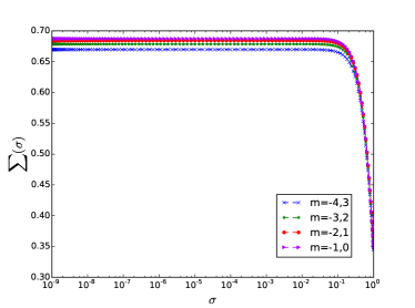
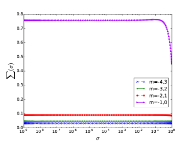
where is the angle between the vectors , with magnitudes and , respectively. In this expression, the cut-off does not appear in the momentum integrations, but in the number of Matsubara frequencies that are summed up. We solve the above equation (12) fixing and appropriately and then recursively search for the solution starting from a given numerical seed. The double numerical integration is performed using Gaussian quadratures, after rescaling the radial component of momentum. In Fig. 1 we show, for the sake of illustration, the solution of the gap equation as a function of the momentum with Matsubara frequencies at two different temperatures and the same fixed value of . We observe that when is close to zero (left panel), every mass function has almost the same height as , but the larger the temperature, the height of all diminishes, except for the corresponding to (right panel).
Once we are able to identify a stable solution for each , we explore the behavior of the chiral condensate, which is the order parameter for the chiral transition and is defined as
| (13) | |||||
This condensate is finite when chiral symmetry is broken, and vanishes when this symmetry is restored. The value of at which this happens is , the critical temperature for the chiral symmetry restoration.
IV Chiral symmetry breaking at finite and constant mass approximation
Because chiral symmetry breaking is an infrared phenomenon, it basically is encoded in the behavior of . Therefore, in the constant mass approximation Ahmad:2015cgh , we replace all mass functions involved in the SDE with their values at zero momentum. Denoting , the gap equation becomes
| (14) |
In what follows, we select the cut-off such that
| (15) |
and write all temperature scales proportional to multiples of , namely, . Performing momentum integration analytically, we have that
| (16) | |||||
This transcendental equation can be solved self consistently, giving the behavior of each as a function of temperature. Near the critical point, we expect to approach zero. Assuming a linear behavior of near criticality, we have that
| (17) | |||||
For the zeroth Matsubara frequency , the above relation simplifies to
| (18) |
Now, because , it follows that
| (19) | |||||
Because of our assumption that near the critical point the temperature-dependent approaches to zero point perpendicularly, in consistency with the Clausius-Clapeyron criterion, we reach to the equality ():
| (20) |
Summation over is finite for every value of temperature, which allow us to obtain the behavior of the critical coupling for each . Considering a cutoff , the behavior of the critical coupling as a function of can be observed in Fig. 2.
The critical coupling can also be obtained from the chiral condensate, which in this approximations reads
| (21) | |||||
In the same Fig. 2, a comparison is shown between the values of derived from Eqs. (20) and (LABEL:condcma), with a qualitative agreement. A fit to this behavior is of the form
| (23) |
This behavior is in disagreement with the finding of Ref. Nascimento:2015ola , which establishes that
| (24) |
As , the last expression is inconsistent with the zero temperature value of the critical coupling .
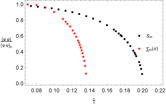
Next, maintaining the fixed value of and taking , in Fig. 3 we show the behavior of the normalized condensate as a function of . We also compare the findings of the condensate including the full momentum dependence of the mass functions. We observe that the number of Matsubara frequencies taken into account is enough to reproduce the correct physical behavior expected for the condensate, namely, it approaches the vertical axis roughly as a constant at small temperature, whereas it hits the horizontal axis with a vertical line as approaches to the critical temperature. The difference of the for both the approximations is due to the static nature of the CMA.
Moreover, fixing the value of the temperature, the condensate as a function of the coupling is depicted in Fig. 4. Results from SDE and CMA are in qualitative agreement, namely, in both cases the condensate starts rising just above and saturate at large . The difference of the for this to happen is due to the nature of CMA.
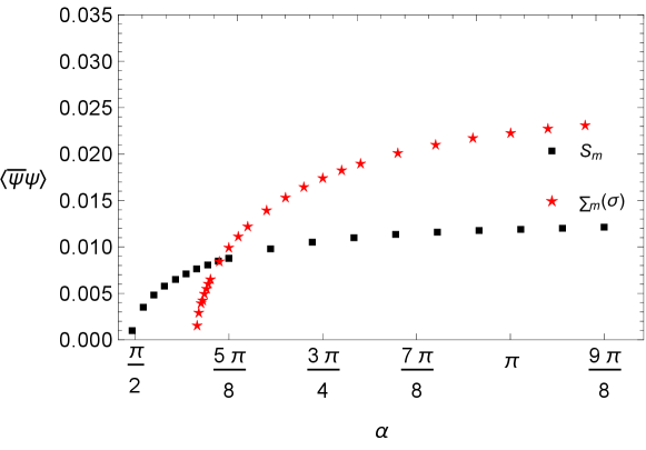
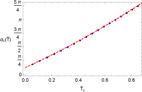
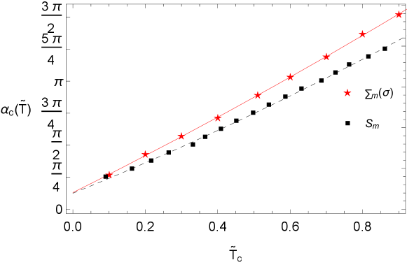
We also depict the critical coupling as a function of from these condensates in Fig. 5. The behavior is qualitatively the same and the error of the CMA does not exceed a few percent in the range of temperatures of our framework as compare with the full SDE prediction. The behavior remains quadratic, of the form
| (25) |
for the CMA (dashed curve) and
| (26) |
for (solid curve).
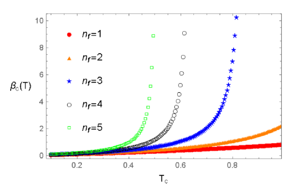
If we consider vacuum polarization effect Gorbar:2001qt , we show the effective coupling as a function of temperature for different fermion families in figure 6.
| (27) |
V Conclusions
In this article, we have revisited the behavior of chiral symmetry restoration in RQED in a heat bath. First, we have computed the critical coupling for chiral symmetry breaking by solving the SDE numerically. Then, the critical temperature is obtained at the point in parameter space in the supercritical regime where the chiral condensate vanishes. We have further approximated the solution to the gap equation in the so-called constant mass approximation by neglecting any momentum dependence of the mass function and taking into account only their IR value. Neither of these numerical solutions agree with the behavior predicted by Nascimento:2015ola . Our numerical procedure shows that there is no critical behavior for none of the values of the cutoff. Instead, the behavior of the critical coupling behaves as a second order polynomial of Temperature. Furthermore, in the limit , the predicted critical coupling for the momentum dependent mass coincides with the critical coupling predicted within the CMA. Extensions to this work are currently under consideration by adding vacuum polarization effects and a chemical potential. Results shall be reported elsewhere.
Acknowledgements.
The authors would like to thank Valery P. Gusynin for valuable comments. JCR acknowledges support from FONDECYT (Chile) under Grant No. 1170107.References
- (1) G. ’t Hooft, Adv. Ser. Math. Phys. 19, 1-683 (1994).
- (2) J. Donoghue, E. Golowich and B. R. Holstein, Camb. Monogr. Part. Phys. Nucl. Phys. Cosmol. 2, 1-540 (1992).
- (3) J. S. Schwinger, Phys. Rev. 128, 2425-2429 (1962).
- (4) G. ’t Hooft, Nucl. Phys. B 75, 461-470 (1974).
- (5) R. Maartens. Living Rev. Rel. 7, 7 (2004).
- (6) R. Maartens and K. Koyama. Living Rev. Rel. 13, 5 (2010).
- (7) P. Brax and C. van de Bruck. Class. Quant. Grav. 20, R201-R232 (2003).
- (8) P. Brax, C. van de Bruck and A. C. Davis. Rept. Prog. Phys. 67, 2183-2232 (2004).
- (9) C. V. Johnson. [arXiv:hep-th/0007170 [hep-th]].
- (10) P. R. Wallace, Phys. Rev. 71 (9): 622–634 (1947).
- (11) Novoselov K S, Geim A K, Morozov S V, Jiang D, Zhang Y, Dubonos S V, Grigorieva I V and Firsov A A Science 306 666 (2004).
- (12) Novoselov K S, Geim A K, Morozov S V, Jiang D, Katsnelson M I, Grigorieva I V, Dubonos S V and Firsov A A, Nature 438, 197–200 (2005).
- (13) Zhang Y, Tan Y-W, Horst L S and Kim P, Nature 438 201 (2005).
- (14) E. Marino, Nucl. Phys. B 408, 551-564 (1993)
- (15) E. Gorbar, V. Gusynin and V. Miransky, Phys. Rev. D 64, 105028 (2001).
- (16) S. Teber, Phys. Rev. D 86, 025005 (2012).
- (17) A. Kotikov and S. Teber, Phys. Rev. D 87, no.8, 087701 (2013).
- (18) A. Kotikov and S. Teber, Phys. Rev. D 89, no.6, 065038 (2014).
- (19) S. Teber and A. Kotikov, EPL 107, no.5, 57001 (2014).
- (20) S. Teber and A. Kotikov, Theor. Math. Phys. 190, no.3, 446-457 (2017).
- (21) S. Teber and A. Kotikov, Phys. Rev. D 97, no.7, 074004 (2018).
- (22) S. Teber and A. Kotikov, JHEP 07, 082 (2018).
- (23) A. Kotikov and S. Teber, Phys. Part. Nucl. 50, no.1, 1-41 (2019).
- (24) A. Ahmad, J. J. Cobos-Martínez, Y. Concha-Sánchez and A. Raya, Phys. Rev. D 93, no.9, 094035 (2016) doi:10.1103/PhysRevD.93.094035 [arXiv:1604.03886 [hep-ph]].
- (25) A. Kotikov, V. Shilin and S. Teber, Phys. Rev. D 94, no.5, 056009 (2016).
- (26) A. Kotikov and S. Teber, Phys. Rev. D 94, no.11, 114010 (2016).
- (27) V. Alves, W. S. Elias, L. O. Nascimento, V. Juričić and F. Peña, Phys. Rev. D 87, no.12, 125002 (2013).
- (28) L. O. Nascimento, V. Alves, F. Peña, C. M. Smith and E. Marino, Phys. Rev. D 92, 025018 (2015).
- (29) A. Ahmad, A. Ayala, A. Bashir, E. Gutiérrez and A. Raya, J. Phys. Conf. Ser. 651, no.1, 012018 (2015) doi:10.1088/1742-6596/651/1/012018