This paper was converted on www.awesomepapers.org from LaTeX by an anonymous user.
Want to know more? Visit the Converter page.

Choosing the pp in LpL_{p} loss: rate adaptivity on the symmetric location problem

Yu-Chun Kao, Min Xu, and Cun-Hui Zhang
Department of Statistics
Rutgers University, New Brunswick, NJ, USA
Corresponding author: Min Xu, Department of Statistics, Rutgers University, New Brunswick, NJ, USA (email: mx76@stat.rutgers.edu)
(July 30, 2025)
Abstract

Given univariate random variables Y1,,YnY_{1},\ldots,Y_{n} distributed uniformly on [θ01,θ0+1][\theta_{0}-1,\theta_{0}+1], the sample midrange Y(n)+Y(1)2\frac{Y_{(n)}+Y_{(1)}}{2} is the MLE for the location parameter θ0\theta_{0} and has estimation error of order 1/n1/n, which is much smaller compared with the 1/n1/\sqrt{n} error rate of the usual sample mean estimator. However, the sample midrange performs poorly when the data has say the Gaussian N(θ0,1)N(\theta_{0},1) distribution, with an error rate of 1/logn1/\sqrt{\log n}. In this paper, we propose an estimator of the location θ0\theta_{0} with a rate of convergence that can, in many settings, adapt to the underlying distribution which we assume to be symmetric around θ0\theta_{0} but is otherwise unknown. When the underlying distribution is compactly supported, we show that our estimator attains a rate of convergence of n1αn^{-\frac{1}{\alpha}} up to polylog factors, where the rate parameter α\alpha can take on any value in (0,2](0,2] and depends on the moments of the underlying distribution. Our estimator is formed by minimizing the LγL_{\gamma}-loss with respect to the data, for a power γ2\gamma\geq 2 chosen in a data-driven way – by minimizing a criterion motivated by the asymptotic variance. Our approach can be directly applied to the regression setting where θ0\theta_{0} is a function of observed features and motivates the use of LγL_{\gamma} loss function with a data-driven γ\gamma in certain settings.

1 Introduction

Given random variables Y1,,YndUniform(θ01,θ0+1)Y_{1},\ldots,Y_{n}\stackrel{{\scriptstyle d}}{{\sim}}\text{Uniform}(\theta_{0}-1,\theta_{0}+1), the optimal estimator for the center θ0\theta_{0} is not the usual sample mean Y¯\bar{Y} but rather the sample midrange Ymid=Y(n)+Y(1)2Y_{\text{mid}}=\frac{Y_{(n)}+Y_{(1)}}{2}, which is also the MLE. Indeed, we have that

𝔼|Y(n)+Y(1)2θ0|\displaystyle\mathbb{E}\biggl{|}\frac{Y_{(n)}+Y_{(1)}}{2}-\theta_{0}\biggr{|} 𝔼|Y(n)θ012|+𝔼|Y(1)θ0+12|\displaystyle\leq\mathbb{E}\biggl{|}\frac{Y_{(n)}-\theta_{0}-1}{2}\biggr{|}+\mathbb{E}\biggl{|}\frac{Y_{(1)}-\theta_{0}+1}{2}\biggr{|}
=1𝔼Y(n)θ02+𝔼Y(1)θ02=2n+1,\displaystyle=1-\mathbb{E}\frac{Y_{(n)}-\theta_{0}}{2}+\mathbb{E}\frac{Y_{(1)}-\theta_{0}}{2}=\frac{2}{n+1},

which is far smaller than the 1/n1/\sqrt{n} error of the sample mean; a two points argument in Le Cam (1973) shows that the 1/n1/n rate is optimal in this case. One may also show via the Lehman–Scheffe Theorem that sample midrange is the uniformly minimum variance unbiased (UMVU) estimator. However, sample midrange is a poor choice when Y1,,YndN(θ0,1)Y_{1},\ldots,Y_{n}\stackrel{{\scriptstyle d}}{{\sim}}N(\theta_{0},1), where we have that 𝔼|Ymidθ0|\mathbb{E}|Y_{\text{mid}}-\theta_{0}| is of order 1/logn1/\sqrt{\log n}. These observations naturally motivate the following question: let pp be a univariate density symmetric around 0 and suppose Y1,,YnY_{1},\ldots,Y_{n} has the distribution p(θ0)p(\,\cdot-\theta_{0}) which is the location shift of pp, can we construct an estimator of the location θ0\theta_{0} whose rate of convergence adapts to the unknown underlying distribution pp?

This question has not yet been addressed by the wealth of existing knowledge, dating back to at least Stein (1956), on symmetric location estimation, which focuses on semiparametric efficiency for asymptotically Normal estimators. The classical theory states that when the underlying density pp is regular in the sense of being differentiable in quadratic mean (DQM), there exists n\sqrt{n}-consistent estimator which has the same asymptotic variance as the best estimator when one does know the underlying density pp; in other words, under the regular regime and in terms of asymptotic efficiency, one can perfectly adapt to the unknown distribution. The adaptive estimators rely on being able to consistently estimate the unknown density at an appropriate rate.

In contrast, the setting where θ0\theta_{0} can be estimated at a rate faster than n\sqrt{n} is irregular in that the Fisher information is infinity and any n\sqrt{n}-asymptotically Normal estimator is suboptimal; the underlying distribution is not DQM and is difficult to estimate. Even the problem of choosing between only the sample mean Y¯\bar{Y} and the sample midrange YmidY_{\text{mid}} is nontrivial, as we show in this paper that tried-and-true method of cross-validation fails in this setting (see Remark 2.1 for the detailed discussion).

If the underlying density pp is known, the optimal rate in estimating the location θ0\theta_{0} is governed by how quickly the function ΔH(p(),p(Δ))\Delta\mapsto H\bigl{(}p(\cdot),p(\cdot-\Delta)\bigr{)} decreases as Δ\Delta goes to zero, where H(p,q):={(p(x)q(x))2𝑑x}1/2H(p,q):=\bigl{\{}\int(\sqrt{p(x)}-\sqrt{q(x)})^{2}dx\bigr{\}}^{1/2} is the Hellinger distance. To be precise, for any estimator θ^\widehat{\theta}, we have

lim infnsupθ0𝔼θ0{nH(p(θ0),p(θ^))}>0,\liminf_{n\rightarrow\infty}\sup_{\theta_{0}}\mathbb{E}_{\theta_{0}}\bigl{\{}\sqrt{n}H\bigl{(}p(\cdot-\theta_{0}),p(\,\cdot-\widehat{\theta})\bigr{)}\bigr{\}}>0,

where the supremum can be taken in a local ball of shrinking radius around any point in \mathbb{R}; see for example Theorem 6.1 of Chapter I of Ibragimov and Has’ Minskii (2013) for an exact statement. Le Cam (1973) also showed that the MLE attains this convergence rate under mild conditions. Therefore, if H2(p(),p(Δ))H^{2}\bigl{(}p(\cdot),p(\cdot-\Delta)\bigr{)} is of order |Δ|α|\Delta|^{\alpha} for some α>0\alpha>0, then the optimal rate of the error 𝔼θ0|θ^θ0|\mathbb{E}_{\theta_{0}}|\widehat{\theta}-\theta_{0}| is n1αn^{-\frac{1}{\alpha}}. If the underlying density pp is DQM, then we have that α=2\alpha=2 which yields the usual rate of n12n^{-\frac{1}{2}}. But, if pp is the uniform density on [1,1][-1,1], we have α=1\alpha=1 which gives an optimal rate of n1n^{-1}.

The behavior of the function ΔH(p(),p(Δ))\Delta\mapsto H\bigl{(}p(\cdot),p(\cdot-\Delta)\bigr{)} depends on the smoothness of the underlying density pp. In the extreme case where pp has a Dirac delta point mass at 0 for instance, H(p(),p(Δ))H\bigl{(}p(\cdot),p(\cdot-\Delta)\bigr{)} is bounded away from 0 for any Δ>0\Delta>0. This is expected since, in this case, we can estimate θ0\theta_{0} perfectly by localizing the discrete point mass. More generally, discontinuities in the density function or singularities in its first derivative anywhere can increase H(p(),p(Δ))H\bigl{(}p(\cdot),p(\cdot-\Delta)\bigr{)} and thus lead to a faster rate in estimating the location θ0\theta_{0}. Interested readers can find a detailed discussion and a large class of examples in Chapter VI of Ibragimov and Has’ Minskii (2013).

When the underlying density pp is unknown, it becomes unclear how to design a rate adaptive location estimator. One possible approach is to nonparametrically estimate pp, but we would need our density estimator to be able to accurately recover the points of discontinuities in pp or singularities in pp^{\prime} – this goes beyond the scope of existing theory on nonparametric density estimation which largely deals with estimating a smooth density pp. Because of the clear difficulty in analyzing rate adaptive location estimation problem in its fullest generality, we focus on rate adaptivity among compactly supported densities which exhibit discontinuity or singularity at the boundary points of the support; the uniform density on [1,1][-1,1] for instance has discontinuity at the boundary points 1-1 and 11.

With the more precise goal in mind, we study a simple class of estimators of the form θ^γ=argminθi=1n|Yiθ|γ\widehat{\theta}_{\gamma}=\operatorname*{arg\,min}_{\theta}\sum_{i=1}^{n}|Y_{i}-\theta|^{\gamma} where the power γ2\gamma\geq 2 is selected in a data-driven way. Estimators of this form encompass both the sample mean Y¯\bar{Y}, with γ=2\gamma=2, and the sample midrange, with γ\gamma\rightarrow\infty. These estimators are easy to interpret, easy to compute, and can be extended in a straightforward way to the regression setting where θ0\theta_{0} is a linear function of some observed covariates.

The key step is selecting the optimal power γ\gamma from the data; in particular, γ\gamma must be allowed to diverge with nn in order for the resulting estimator to have an adaptive rate. Since θ^γ\widehat{\theta}_{\gamma} is unbiased for any γ2\gamma\geq 2, the ideal selection criterion is to minimize the variance. In this work, we approximate the variance of θ^γ\widehat{\theta}_{\gamma} by its asymptotic variance, which has a finite sample empirical analog that can be computed from the empirical central moments of the data. We then select γ\gamma by minimizing the empirical asymptotic variance, using Lepski’s method to ensure that we consider only those γ\gamma’s for which the empirical asymptotic variance is a good estimate of the population version. For any distribution with a finite second moment, the resulting estimator has rate of convergence at least as fast as O~(n1/2)\widetilde{O}(n^{-1/2}), where we use the O~()\widetilde{O}(\cdot) notation to suppress log-factors. Moreover, for any compacted supported density pp that satisfies a moment condition of the form |z|γp(z)𝑑zγα\int|z|^{\gamma}p(z)\,dz\asymp\gamma^{-\alpha} for some α(0,2]\alpha\in(0,2], our estimator attains an adaptive rate of O~(n1α)\widetilde{O}(n^{-\frac{1}{\alpha}}).

Our estimation procedure can be easily adapted to the linear regression setting where we have Yi=Xiβ0+ZiY_{i}=X_{i}^{\top}\beta_{0}+Z_{i} where ZiZ_{i} has a distribution symmetric around 0. It is computationally fast using second order methods and can be directly applied on real data. Importantly, it is robust to violation of the symmetry assumption. More precisely, if Yi=θ0+ZiY_{i}=\theta_{0}+Z_{i} and the noise ZiZ_{i} has a distribution that is asymmetric around 0 but still has mean zero, then our estimator will converge to 𝔼Yi=θ0\mathbb{E}Y_{i}=\theta_{0} nevertheless.

The rest of our paper is organized as follows: we finish Section 1 reviewing existing work and defining commonly used notation. In Section 2, we formally define the problem and our proposed method; we also show that our proposed method has a rate of convergence that is at least O~(n12)\widetilde{O}(n^{-\frac{1}{2}}) (Theorem 2.1). In Section 3, we prove that our proposed estimator has an adaptive rate of convergence O~(n1α)\widetilde{O}(n^{-\frac{1}{\alpha}}) where α(0,2]\alpha\in(0,2] is determined by a moment condition on the noise distribution. We perform empirical studies in Section 4 and conclude with a discussion of open problems in Section 5.

1.1 Literature review

Starting from the seminal paper by Stein (1956), a long series of work, for example Stone (1975)Beran (1978), and many others (Van Eeden, 1970; Bickel, 1982; Schick, 1986; Mammen and Park, 1997; Dalalyan et al., 2006) showed, under the regular DQM setting, we can attain an asymptotically efficient estimator θ^\widehat{\theta} by taking a pilot estimator θ^init\widehat{\theta}_{\text{init}}, applying a density estimation method on the residues Z~i=Yiθ^init\widetilde{Z}_{i}=Y_{i}-\widehat{\theta}_{\text{init}} to obtain a density estimate p^\widehat{p}, and then construct θ^\widehat{\theta} either by maximizing the estimated log-likelihood, by taking one Newton step using an estimate of the Fisher information, or by various other related schemes; see Bickel et al. (1993) for more discussion on adaptive efficiency. Interestingly, Laha (2021) recently showed that the smoothness assumption can be substituted by a log-concavity condition instead.

Also motivated in part by the contrast between sample midrange and sample mean, Baraud et al. (2017) and Baraud and Birgé (2018) propose the ρ\rho-estimator. When the underlying density pp is known, the ρ\rho-estimator has optimal rate in estimating the location. When pp is unknown, the ρ\rho-estimator would need to estimate pp nonparametrically; it is not clear under what conditions it would attain adaptive rate. Moreover, computing the ρ\rho-estimator in practice is often difficult.

Our estimator is related to methods in robust statistics (Huber, 2011), although our aim is different. Our asymptotic variance based selector can be seen as a generalization of a procedure proposed by Lai et al. (1983), which uses the asymptotic variance to select between the sample mean and the median. Another somewhat related line of work is that of Chierichetti et al. (2014) and Pensia et al. (2019), which study location estimation when Z1,,ZnZ_{1},\ldots,Z_{n} are allowed to have different distributions, all of which are still symmetric around 0, and construct robust estimators that interestingly adapt to the heterogeneity of the distributions of the ZiZ_{i}’s.

1.2 Notation

We write [n]:={1,2,,n}[n]:=\{1,2,\ldots,n\}. We write ab:=min(a,b)a\wedge b:=\min(a,b), ab:=max(a,b)a\vee b:=\max(a,b), (a)+:=a0(a)_{+}:=a\vee 0 and (a):=(a0)(a)_{-}:=-(a\wedge 0). For two functions f,gf,g, we write fgf\gtrsim g if there exists a universal constant C>0C>0 such that fCgf\geq Cg; we write fgf\asymp g or fgf\propto g if fgf\gtrsim g and gfg\gtrsim f. We use CC to denote a positive universal constants whose value may be different from instance to instance. We use the O~()\widetilde{O}(\cdot) notation to represent rate of convergence ignoring poly-log factors.

2 Method

We observe random variables Y1,,YnY_{1},\ldots,Y_{n} such that

Yi=θ0+Zi for i[n]Y_{i}=\theta_{0}+Z_{i}\text{ for $i\in[n]$}

where θ0\theta_{0}\in\mathbb{R} is the unknown location and Z1,,ZndPZ_{1},\ldots,Z_{n}\stackrel{{\scriptstyle d}}{{\sim}}P where PP is an unknown distribution with density p()p(\cdot) symmetric around zero. Our goal is to estimate θ0\theta_{0} from the observations Y1,,YnY_{1},\ldots,Y_{n}.

2.1 A simple class of estimators

Our approach is motivated by the fact that both the sample mean and the sample midrange minimize the γ\ell^{\gamma} norm of the residual for different values of γ\gamma. More precisely,

Y¯\displaystyle\bar{Y} :=1ni=1nYi=argminθi=1n|Yiθ|2, and\displaystyle:=\frac{1}{n}\sum_{i=1}^{n}Y_{i}=\operatorname*{arg\,min}_{\theta\in\mathbb{R}}\sum_{i=1}^{n}|Y_{i}-\theta|^{2},\quad\text{ and }
Ymid\displaystyle Y_{\text{mid}} :=Y(n)+Y(1)2=argminθmaxi[n]|Yiθ|=limγargminθi=1n|Yiθ|γ.\displaystyle:=\frac{Y_{(n)}+Y_{(1)}}{2}=\operatorname*{arg\,min}_{\theta\in\mathbb{R}}\max_{i\in[n]}|Y_{i}-\theta|=\lim_{\gamma\rightarrow\infty}\operatorname*{arg\,min}_{\theta\in\mathbb{R}}\sum_{i=1}^{n}|Y_{i}-\theta|^{\gamma}.

This suggests an estimation scheme where we first select the power γ2\gamma\geq 2 in a data-driven way and then output the empirical center with respect to the γ\ell^{\gamma} norm:

θ^γ:=argminθi=1n|Yiθ|γ.\widehat{\theta}_{\gamma}:=\operatorname*{arg\,min}_{\theta\in\mathbb{R}}\sum_{i=1}^{n}|Y_{i}-\theta|^{\gamma}.

It is clear that Y¯=θ^2\bar{Y}=\widehat{\theta}_{2} and that θ^γ\widehat{\theta}_{\gamma} approaches YmidY_{\text{mid}} as γ\gamma increases, that is, Ymidθ^:=limγθ^γY_{\text{mid}}\equiv\widehat{\theta}_{\infty}:=\lim_{\gamma\rightarrow\infty}\widehat{\theta}_{\gamma}. We in fact have a deterministic bound of |θ^γYmid||\widehat{\theta}_{\gamma}-Y_{\text{mid}}| in the following lemma:

Lemma 1.

Let Y1,,YnY_{1},\ldots,Y_{n} be nn arbitrary points on \mathbb{R}, then

|θ^γYmid|2(Y(n)Y(1))lognγ.|\widehat{\theta}_{\gamma}-Y_{\text{mid}}|\leq 2(Y_{(n)}-Y_{(1)})\frac{\log n}{\gamma}.

We prove Lemma 1 in Section S1 of the appendix. It is important to note that, by Lemma 1, we need to consider γ\gamma as large as nn to approximate YmidY_{\text{mid}} with error that is of order lognn\frac{\log n}{n}. Therefore, in settings where YmidY_{\text{mid}} is optimal, we need γ\gamma to be able to diverge with nn.

Estimators of form θ^γ\widehat{\theta}_{\gamma} is simple, easy to compute via Newton’s method (see Section S1.4 of the appendix), and interpretable even for asymmetric distributions. The key question is of course, how do we select the power γ\gamma? It is necessary to allow γ\gamma to increase with nn to attain adaptive rate but selecting a power γ\gamma that is too large can introduce tremendous excess variance. As is often said, ”with great power comes great responsibility”.

Before describing our approach in the next subsection, we give some remarks on two approaches that seem reasonable but in fact have significant limitations.

Remark 2.1.

(Suboptimality of Cross-validation)
Cross-validation is a natural method for choosing the best estimator among some family, but this fails in our problem. To illustrate why, we consider the simpler problem where we choose between only the sample mean θ^2\widehat{\theta}_{2} and the sample midrange θ^\widehat{\theta}_{\infty}. We consider held-out validation where we divide our data into training data DtrainD^{\text{train}} and test data DtestD^{\text{test}} each with nn data points. We compute θ^2train,θ^train\widehat{\theta}_{2}^{\text{train}},\widehat{\theta}_{\infty}^{\text{train}} on training data, evaluate test data MSE

R^(θ^2train):=1ni=1n(Yitestθ^2train)2=1ni=1n(YitestY¯test)2+(Y¯testθ^2train)2,\displaystyle\widehat{R}(\widehat{\theta}_{2}^{\text{train}}):=\frac{1}{n}\sum_{i=1}^{n}(Y^{\text{test}}_{i}-\widehat{\theta}_{2}^{\text{train}})^{2}=\frac{1}{n}\sum_{i=1}^{n}(Y^{\text{test}}_{i}-\bar{Y}^{\text{test}})^{2}+(\bar{Y}^{\text{test}}-\widehat{\theta}_{2}^{\text{train}})^{2}, (1)

for θ^2train\widehat{\theta}^{\text{train}}_{2} and also R^(θ^train)\widehat{R}(\widehat{\theta}_{\infty}^{\text{train}}) for the θ^train\widehat{\theta}_{\infty}^{\text{train}} midrange estimator. Since the first term on the right hand side of (1) is constant, we select γ=2\gamma=2 if (Y¯testθ^2train)2<(Y¯testθ^train)2(\bar{Y}^{\text{test}}-\widehat{\theta}_{2}^{\text{train}})^{2}<(\bar{Y}^{\text{test}}-\widehat{\theta}_{\infty}^{\text{train}})^{2}.

Now assume that the data follows the uniform distribution on [θ01,θ0+1][\theta_{0}-1,\theta_{0}+1], so that the optimal estimator is the sample midrange θ^\widehat{\theta}_{\infty}. We observe that n(θ^2trainθ0)dN(0,1/3)\sqrt{n}(\widehat{\theta}_{2}^{\text{train}}-\theta_{0})\stackrel{{\scriptstyle d}}{{\rightarrow}}N(0,1/3) and n(Y¯testθ0)dN(0,1/3)\sqrt{n}(\bar{Y}^{\text{test}}-\theta_{0})\stackrel{{\scriptstyle d}}{{\rightarrow}}N(0,1/3) whereas n(θ^trainθ0)0\sqrt{n}(\widehat{\theta}_{\infty}^{\text{train}}-\theta_{0})\rightarrow 0 in probability. Hence, by the Portmanteau Theorem,

lim infn(selecting θ^2)\displaystyle\liminf_{n\rightarrow\infty}\mathbb{P}(\text{selecting $\widehat{\theta}_{2}$}) =lim infn(|Y¯testθ^2train|<|Y¯testθ^train|)\displaystyle=\liminf_{n\rightarrow\infty}\mathbb{P}(|\bar{Y}^{\text{test}}-\widehat{\theta}_{2}^{\text{train}}|<|\bar{Y}^{\text{test}}-\widehat{\theta}_{\infty}^{\text{train}}|)
=lim infn(|n(Y¯testθ0)n(θ^2trainθ0)|\displaystyle=\liminf_{n\rightarrow\infty}\mathbb{P}(|\sqrt{n}(\bar{Y}^{\text{test}}-\theta_{0})-\sqrt{n}(\widehat{\theta}_{2}^{\text{train}}-\theta_{0})|
<|n(Y¯testθ0)n(θ^trainθ0)|)\displaystyle\hskip 50.58878pt<|\sqrt{n}(\bar{Y}^{\text{test}}-\theta_{0})-\sqrt{n}(\widehat{\theta}_{\infty}^{\text{train}}-\theta_{0})|)
(|W1W2|<|W2|)>0,\displaystyle\geq\mathbb{P}(|W_{1}-W_{2}|<|W_{2}|)>0,

where W1W_{1} and W2W_{2} are independent N(0,1/3)N(0,1/3) random variables. In other words, held-out validation has a non-vanishing probability of incorrectly selecting θ^2\widehat{\theta}_{2} over θ^\widehat{\theta}_{\infty} even as nn\rightarrow\infty and thus has an error of order 1/n1/\sqrt{n}, which is far larger than the optimal 1/n1/n rate. It is straightforward to extend the argument to the setting of KK-fold cross-validation for any fixed KK.

Remark 2.2.

(Suboptimality of MLE with respect to the generalized Gaussian family)
We observe that θ^γ\widehat{\theta}_{\gamma} is the maximum likelihood estimator for the center when the data follow the Generalized Normal GN(θ,σ,γ)(\theta,\sigma,\gamma) distribution, which is also known as the Subbotin distribution (Subbotin, 1923), whose density is of the form

p(x;θ,σ,γ)=12σΓ(1+1/γ)exp(|xθσ|γ),\displaystyle p(x\,;\,\theta,\sigma,\gamma)=\frac{1}{2\sigma\Gamma(1+1/\gamma)}\exp\biggl{(}-\biggl{|}\frac{x-\theta}{\sigma}\biggr{|}^{\gamma}\biggr{)},

where Γ(t):=0xt1ex𝑑x\Gamma(t):=\int_{0}^{\infty}x^{t-1}e^{-x}dx denotes the Gamma function. This suggests a potential approach where we determine γ\gamma by fitting the data to the potentially misspecified Generalized Gaussian family via likelihood maximization:

argminγminθ,σ1ni=1n|Yiθσ|γ+logσ+log(2Γ(1+1/γ)).\displaystyle\operatorname*{arg\,min}_{\gamma}\min_{\theta,\sigma}\frac{1}{n}\sum_{i=1}^{n}\biggl{|}\frac{Y_{i}-\theta}{\sigma}\biggr{|}^{\gamma}+\log\sigma+\log(2\Gamma(1+1/\gamma)).

This approach works well if the underlying density pp of the noise ZiZ_{i} belongs in the Generalized Gaussian family. Otherwise, it may be suboptimal: it may select a γ\gamma that is too small when the optimal γ\gamma is large and it may select a γ\gamma that is too large when the optimal γ\gamma is small. We give a precise and detailed discussion of the drawbacks of the generalized Gaussian MLE in Section 3.2.

2.2 Asymptotic variance

Under the assumption that the noise ZiZ_{i} has a distribution symmetric around 0, it is easy to see by symmetry that 𝔼θ^γ=θ0\mathbb{E}\widehat{\theta}_{\gamma}=\theta_{0} for any fixed γ>0\gamma>0. We thus propose a selection scheme based on minimizing the variance. The finite sample variance of θ^γ\widehat{\theta}_{\gamma} is intractable to compute, but for any fixed γ>1\gamma>1, assuming 𝔼|Yθ0|2(γ1)<\mathbb{E}|Y-\theta_{0}|^{2({\gamma-1})}<\infty, we have that n(θ^γθ0)dN(0,V(γ))\sqrt{n}(\widehat{\theta}_{\gamma}-\theta_{0})\stackrel{{\scriptstyle d}}{{\to}}N(0,V(\gamma)) as nn\rightarrow\infty, where

V(γ):=𝔼|Yθ0|2(γ1)[(γ1)𝔼|Yθ0|γ2]2\displaystyle V(\gamma):=\frac{\mathbb{E}|Y-\theta_{0}|^{2(\gamma-1)}}{\left[(\gamma-1)\mathbb{E}|Y-\theta_{0}|^{\gamma-2}\right]^{2}} (2)

is the asymptotic variance of θ^γ\widehat{\theta}_{\gamma}. Thus, from an asymptotic perspective, θ^γ\widehat{\theta}_{\gamma} is a better estimator of θ0\theta_{0} if V(γ)V(\gamma) is small. When γ\gamma is allowed to depend on nn, V(γ)V(\gamma) may not be a good approximation of the finite sample variance of θ^γ\widehat{\theta}_{\gamma}, but the next example suggests that V()V(\cdot) is still a sensible selection criterion.

Example 1.

When Y1,,YndUniform[θ01,θ0+1]Y_{1},\ldots,Y_{n}\stackrel{{\scriptstyle d}}{{\sim}}\text{Uniform}[\theta_{0}-1,\theta_{0}+1], straightforward calculation yields that 𝔼|Yθ0|q=1q+1\mathbb{E}|Y-\theta_{0}|^{q}=\frac{1}{q+1} for any qq\in\mathbb{N} and thus, we have V(γ)=12γ1V(\gamma)=\frac{1}{2\gamma-1}. We see that V(γ)V(\gamma) is minimized when γ\gamma\rightarrow\infty, in accordance with the fact that the sample midrange YmidY_{\text{mid}} is the optimal estimator among the class of estimators {θ^γ}γ2\{\widehat{\theta}_{\gamma}\}_{\gamma\geq 2}. More generally, if YiY_{i} has a density p()p(\cdot) supported on [θ01,θ0+1][\theta_{0}-1,\theta_{0}+1] which is symmetric around θ0\theta_{0} and satisfies the property that p(x)p(x) is bounded away from 0 and \infty for all x[θ01,θ0+1]x\in[\theta_{0}-1,\theta_{0}+1], then one may show that V(γ)1γV(\gamma)\propto\frac{1}{\gamma}. On the other hand, if YiN(θ0,1)Y_{i}\sim N(\theta_{0},1), then, using the fact that 𝔼|Yθ0|γγγ/2eγ/2\mathbb{E}|Y-\theta_{0}|^{\gamma}\asymp\gamma^{\gamma/2}e^{-\gamma/2}, we can directly calculate that that V(γ)2γγV(\gamma)\asymp\frac{2^{\gamma}}{\gamma}, which goes to infinity as γ\gamma\rightarrow\infty as expected. Using the fact that θ^2\widehat{\theta}_{2} is the MLE, we have that V(γ)V(\gamma) is minimized at γ=2\gamma=2 in the Gaussian case.

2.3 Proposed procedure

We thus propose to select γ\gamma by minimizing an estimate of the asymptotic variance V(γ)V(\gamma). For simplicity, we restrict our attention to γ2\gamma\geq 2 in the main paper and discuss how to select γ[1,2)\gamma\in[1,2) in Remark 2.6. A natural estimator of V(γ)V(\gamma) is

V^(γ):=minθ1ni=1n|Yiθ|2(γ1)[(γ1)minθ1ni=1n|Yiθ|γ2]2.\displaystyle\widehat{V}(\gamma):=\frac{\min_{\theta}\frac{1}{n}\sum_{i=1}^{n}|Y_{i}-\theta|^{2(\gamma-1)}}{\left[(\gamma-1)\min_{\theta}\frac{1}{n}\sum_{i=1}^{n}|Y_{i}-\theta|^{\gamma-2}\right]^{2}}. (3)

Although V^(γ)\widehat{V}(\gamma) has pointwise consistency in that it is a consistent estimator of V(γ)V(\gamma) for any fixed γ\gamma (see Lemma 2 in Section S1.2 of the appendix), we require uniform consistency since our goal is to minimize V^(γ)\widehat{V}(\gamma) as a surrogate of V(γ)V(\gamma). This unfortunately does not hold; if we allow γ\gamma to diverge with nn, the error |V^(γ)V(γ)||\widehat{V}(\gamma)-V(\gamma)| can be arbitrarily large. This occurs because, if we fix nn and increase γ\gamma, the finite average 1ni=1n|Yiθ|γ\frac{1}{n}\sum_{i=1}^{n}|Y_{i}-\theta|^{\gamma} does not approximate the population mean and behaves closer to 1nmaxi|Yiθ|γ\frac{1}{n}\max_{i}|Y_{i}-\theta|^{\gamma} instead. Indeed, for any fixed nn and any deterministic set of points Y1,,YnY_{1},\ldots,Y_{n}, we have

V^():=limγV^(γ)\displaystyle\widehat{V}(\infty):=\lim_{\gamma\rightarrow\infty}\widehat{V}(\gamma) =limγn(γ1)2|Y(n)Ymid|2(γ1)+|Y(1)Ymid|2(γ1){|Y(n)Ymid|γ2+|Y(1)Ymid|γ2}2\displaystyle=\lim_{\gamma\rightarrow\infty}\frac{n}{(\gamma-1)^{2}}\frac{|Y_{(n)}-Y_{\text{mid}}|^{2(\gamma-1)}+|Y_{(1)}-Y_{\text{mid}}|^{2(\gamma-1)}}{\{|Y_{(n)}-Y_{\text{mid}}|^{\gamma-2}+|Y_{(1)}-Y_{\text{mid}}|^{\gamma-2}\}^{2}}
=limγn2(γ1)2|Y(n)Y(1)2|2=0.\displaystyle=\lim_{\gamma\rightarrow\infty}\frac{n}{2(\gamma-1)^{2}}\biggl{|}\frac{Y_{(n)}-Y_{(1)}}{2}\biggr{|}^{2}=0. (4)

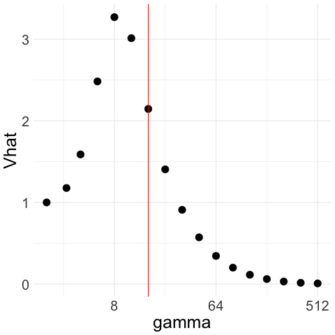
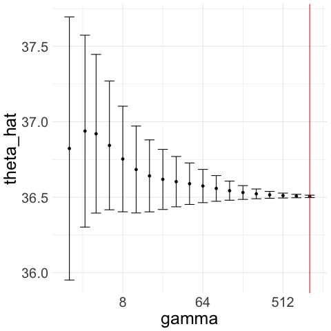
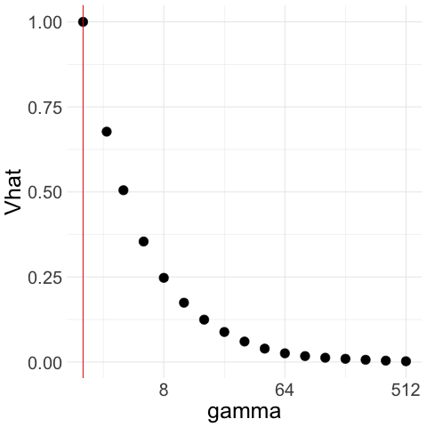
Therefore, unconstrained minimization of V^(γ)\widehat{V}(\gamma) over all γ1\gamma\geq 1 would select γ=\gamma=\infty. See for example Figure 1(a), where we generate Gaussian noise ZiN(0,1)Z_{i}\sim N(0,1) and plot V^(γ)\widehat{V}(\gamma) for a range of γ\gamma’s; although the population V(γ)V(\gamma) tends to infinity when γ\gamma is large, the empirical V^(γ)\widehat{V}(\gamma) increases for moderately large γ\gamma but then, as γ\gamma further increases, V^(γ)\widehat{V}(\gamma) decreases and tends to 0.

Luckily, we can overcome this issue by restricting our attention to γ\gamma’s that are not too large. To be precise, we add an upper bound γmax2\gamma_{\max}\geq 2 and minimize V^(γ)\widehat{V}(\gamma) only among γ[2,γmax]\gamma\in[2,\gamma_{\max}]. We select γmax\gamma_{\max} using Lepski’s method, which is typically used to select smoothing parameters in nonparametric estimation problems (Lepskii, 1990, 1991) but can be readily adapted to our setting. The idea is to construct confidence intervals θ^γ±τV^(γ)/n\widehat{\theta}_{\gamma}\pm\tau\sqrt{\widehat{V}(\gamma)/n} for a set of γ\gamma’s, starting with γ=2\gamma=2, and take γmax\gamma_{\max} to be the largest γ\gamma such that the confidence intervals all intersect. We would thus exclude γ\gamma for which θ^γ\widehat{\theta}_{\gamma} is far from θ0\theta_{0} and V^(γ)\widehat{V}(\gamma) is too small.

This leads to our full estimation procedure below, which we refer to as CAVS (Constrained Asymptotic Variance Selector):

Algorithm 1 Constrained Asymptotic Variance Selection (CAVS) algorithm

Let τ>0\tau>0 be a tuning parameter and let 𝒩n[2,]\mathcal{N}_{n}\subseteq[2,\infty] be the set of candidate γ\gamma’s. Define V^(γ)\widehat{V}(\gamma) as (3) for γ[2,)\gamma\in[2,\infty) and define V^():=0\widehat{V}(\infty):=0.

  1. 1.

    Define γmax\gamma_{\max} as the largest γ𝒩n\gamma\in\mathcal{N}_{n} such that

    γ𝒩n,γγmax[θ^γτV^(γ)n,θ^γ+τV^(γ)n].\displaystyle\bigcap_{\gamma\in\mathcal{N}_{n},\,\gamma\leq\gamma_{\max}}\biggl{[}\widehat{\theta}_{\gamma}-\tau\sqrt{\frac{\widehat{V}(\gamma)}{n}},\,\widehat{\theta}_{\gamma}+\tau\sqrt{\frac{\widehat{V}(\gamma)}{n}}\biggr{]}\neq\emptyset.
  2. 2.

    Select

    γ^:=argminγ𝒩n,γγmaxV^(γ).\widehat{\gamma}:=\operatorname*{arg\,min}_{\gamma\in\mathcal{N}_{n},\,\gamma\leq\gamma_{\max}}\widehat{V}(\gamma).
  3. 3.

    Output

    θ^θ^γ^=argminθi=1n|Yiθ|γ^.\displaystyle\widehat{\theta}\equiv\widehat{\theta}_{\widehat{\gamma}}=\operatorname*{arg\,min}_{\theta\in\mathbb{R}}\sum_{i=1}^{n}|Y_{i}-\theta|^{\widehat{\gamma}}. (5)
Refer to caption
(a) V^(γ)\widehat{V}(\gamma) for Gaussian
Refer to caption
(b) θ^γ±2V^(γ)n\widehat{\theta}_{\gamma}\pm 2\sqrt{\frac{\widehat{V}(\gamma)}{n}}
Refer to caption
(c) V^(γ)\widehat{V}(\gamma) for trunc Gaussian
Refer to caption
(d) θ^γ±2V^(γ)n\widehat{\theta}_{\gamma}\pm 2\sqrt{\frac{\widehat{V}(\gamma)}{n}}
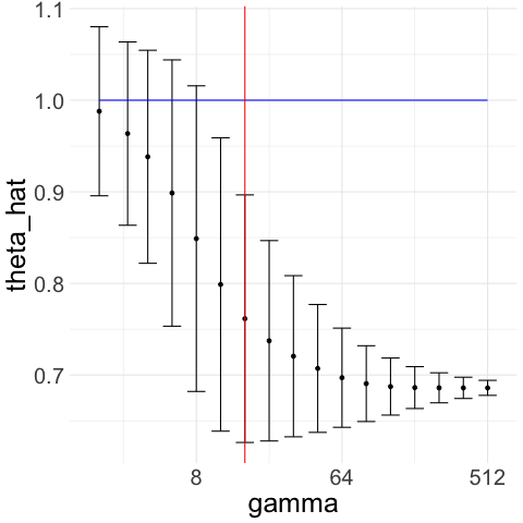
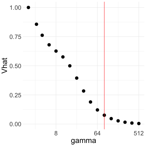
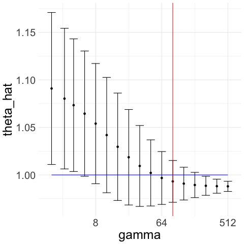
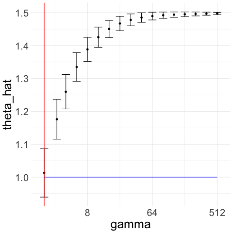
Figure 1: Red vertical line gives γmax\gamma_{\text{max}}; blue horizontal line is the true θ0\theta_{0}. We use n=500n=500. We select γmax\gamma_{\max} as the largest γ\gamma such that all confidence intervals to the left have a nonempty intersection.

The candidate set 𝒩n\mathcal{N}_{n} can be the entire half-line [2,][2,\infty]. In practice, we take 𝒩n\mathcal{N}_{n} to be a finite set so that we are able to compute the minimizer of V^(γ)\widehat{V}(\gamma). A convenient and computationally efficient choice is 𝒩n={2,4,8,,n,}\mathcal{N}_{n}=\{2,4,8,\ldots,n,\infty\}.

We illustrate how the CAVS procedure works with two examples in Figure 1. In Figure 1(a), we generate Gaussian noise ZiN(0,1)Z_{i}\sim N(0,1); we plot V^(γ)\widehat{V}(\gamma) for a exponentially increasing sequence of γ\gamma’s ranging from 2 to 512. The constraint upper bound γmax\gamma_{\max} is given by the red line in the figure. Unconstrained minimization of V^(γ)\widehat{V}(\gamma) leads to γ^=512\widehat{\gamma}=512. Figure 1(b) illustrates the Lepski method that we use to choose upper bound γmax\gamma_{\max}: we compute confidence intervals of width τV^(γ)n\tau\sqrt{\frac{\widehat{V}(\gamma)}{n}} around θ^γ\widehat{\theta}_{\gamma} for the whole range of γ\gamma’s. To get γmax\gamma_{\max}, we pick the largest γ\gamma such that the intersection of all the confidence intervals to the left of γmax\gamma_{\max} is non-empty.

This allows us to avoid the region where V^(γ)\widehat{V}(\gamma) is very small but the actual asymptotic variance V(γ)V(\gamma) is very large. Indeed, if V(γ)V(\gamma) is much larger than the variance Var(Z)\text{Var}(Z), then θ^γ\widehat{\theta}_{\gamma} likely to be quite far from the sample mean θ^2\widehat{\theta}_{2} and thus, if V^(γ)\widehat{V}(\gamma) is also small, then θ^γ±τV^(γ)n\widehat{\theta}_{\gamma}\pm\tau\sqrt{\frac{\widehat{V}(\gamma)}{n}} is unlikely to overlap with the confidence interval around the sample mean.

Therefore, with Gaussian noise, CAVS selects γ^=2\widehat{\gamma}=2 by minimizing V^(γ)\widehat{V}(\gamma) only to the left of γmax\gamma_{\max} (red line) in Figure 1(a). In contrast, if V(γ)V(\gamma) decreases as γ\gamma increases, then θ^γ\widehat{\theta}_{\gamma} remains close to the sample mean θ^2\widehat{\theta}_{2} and the confidence interval θ^γ±τV^(γ)n\widehat{\theta}_{\gamma}\pm\tau\sqrt{\frac{\widehat{V}(\gamma)}{n}} overlaps with that of the sample mean even when γ\gamma is large, which means we would select a large γmax\gamma_{\max} as desired. We illustrate this in Figure 1(c) and 1(d), where we generate truncated Gaussian noise ZZ by truncating at |Z|2|Z|\leq 2; that is, we generate Gaussian samples and keep only those that lie in the interval [2,2][-2,2]. In this case, the optimal γ\gamma is γ=\gamma=\infty and the optimal rate is 1/n1/n. From Figure 1(c), we see that our procedure picks a large γ^=128\widehat{\gamma}=128.

Remark 2.3.

(Selecting τ\tau parameter)

Our proposed CAVS procedure has a tuning parameter τ\tau which governs the strictness of the γmax\gamma_{\max} constraint. Smaller τ\tau will in general result in a smaller γmax\gamma_{\max} and hence a stronger constraint. For our theoretical results, namely Theorem 3.1, it suffices to choose τ\tau to be very slowly growing so that τloglogn\frac{\tau}{\sqrt{\log\log n}}\rightarrow\infty. For practical data analysis applications, we recommend τ=1\tau=1 as a conservative choice based on simulation studies in Section 4.1

Remark 2.4.

(Robustness to asymmetry)

One important aspect of CAVS is that it is robust to violations of the symmetry assumption. If the density pp of the noise ZiZ_{i} has mean zero but is asymmetric (so that θ0\theta_{0} is the mean of YiY_{i}), then, for various γ\gamma’s that are greater than 2, the γ\gamma-th center of Yi=θ0+ZiY_{i}=\theta_{0}+Z_{i} may be different from θ0\theta_{0}; that is θγ:=argminθ𝔼|Yθ|γθ0\theta^{*}_{\gamma}:=\operatorname*{arg\,min}_{\theta}\mathbb{E}|Y-\theta|^{\gamma}\neq\theta_{0} so that θ^γ\widehat{\theta}_{\gamma} is a biased estimator of θ0\theta_{0}. In such cases however, the confidence interval θ^γ±τV^(γ)n\widehat{\theta}_{\gamma}\pm\tau\sqrt{\frac{\widehat{V}(\gamma)}{n}} will, for large enough nn, be concentrated around 𝔼θ^γ=θγ\mathbb{E}\widehat{\theta}_{\gamma}=\theta^{*}_{\gamma} and thus not overlap with the confidence interval about the sample mean θ^2±τV^(2)n\widehat{\theta}_{2}\pm\tau\sqrt{\frac{\widehat{V}(2)}{n}}, which will concentrated around 𝔼θ^2=θ0\mathbb{E}\widehat{\theta}_{2}=\theta_{0}. Therefore, we would have γmax<γ\gamma_{\max}<\gamma and the constraint would thus exclude any biased θ^γ\widehat{\theta}_{\gamma}. We illustrate an example in Figure 2 where because θ^3\widehat{\theta}_{3} is biased, we have that γmax=2\gamma_{\max}=2 and thus, we select γ^=2\widehat{\gamma}=2 and the resulting estimator θ^γ^\widehat{\theta}_{\widehat{\gamma}} still converges to θ0\theta_{0}. Indeed, our basic convergence guarantee–formalized in Theorem 2.1–does not require the noise distribution to be symmetric around 0, it only requires the noise to have mean zero.
Refer to caption
(a) V^\widehat{V} for asymmetric density
Refer to caption
(b) θ^γ±2V^(γ)n\widehat{\theta}_{\gamma}\pm 2\sqrt{\frac{\widehat{V}(\gamma)}{n}}
Figure 2: We generate mean zero ZiZ_{i} from an asymmetric mixture distribution 23Unif[1,0]+13Unif[0,2]\frac{2}{3}\text{Unif}[-1,0]+\frac{1}{3}\text{Unif}[0,2]. Note that θ^3±2V^(3)n\widehat{\theta}_{3}\pm 2\sqrt{\frac{\widehat{V}(3)}{n}} does not overlap with θ^2±2V^(2)n\widehat{\theta}_{2}\pm 2\sqrt{\frac{\widehat{V}(2)}{n}} because 𝔼θ^2𝔼θ^3\mathbb{E}\widehat{\theta}_{2}\neq\mathbb{E}\widehat{\theta}_{3} due to the asymmetry. Red vertical line gives γmax\gamma_{\text{max}}; blue horizontal line is the true θ0\theta_{0}.
Remark 2.5.

(Extension to the regression setting)

We can directly extend our estimation procedure to the linear regression setting. Suppose we observe (Yi,Xi)(Y_{i},X_{i}) for i=1,2,,ni=1,2,\ldots,n where XiX_{i} is a random vector on d\mathbb{R}^{d}, Yi=Xiβ0+ZiY_{i}=X_{i}^{\top}\beta_{0}+Z_{i}, and ZiZ_{i} is an independent noise with a distribution symmetric around 0.

Then, we would compute, for each γ\gamma in a set 𝒩n[2,]\mathcal{N}_{n}\subset[2,\infty],

β^γ\displaystyle\widehat{\beta}_{\gamma} =argminβpi=1n|YiXiβ|γ and\displaystyle=\operatorname*{arg\,min}_{\beta\in\mathbb{R}^{p}}\sum_{i=1}^{n}|Y_{i}-X_{i}^{\top}\beta|^{\gamma}\quad\text{ and }
V^(γ)\displaystyle\widehat{V}(\gamma) =minβd1ni=1n|YiXiβ|2(γ1)(γ1)2{minβd1ni=1n|YiXiβ|γ2}2.\displaystyle=\frac{\min_{\beta\in\mathbb{R}^{d}}\frac{1}{n}\sum_{i=1}^{n}|Y_{i}-X_{i}^{\top}\beta|^{2(\gamma-1)}}{(\gamma-1)^{2}\{\min_{\beta\in\mathbb{R}^{d}}\frac{1}{n}\sum_{i=1}^{n}|Y_{i}-X_{i}^{\top}\beta|^{\gamma-2}\}^{2}}.

We define Σ^X:=1ni=1nXiXi\widehat{\Sigma}_{X}:=\frac{1}{n}\sum_{i=1}^{n}X_{i}X_{i}^{\top}. Using Taylor expansion, it is straightforward to show that nΣ^X1/2(β^γβ0)dN(0,V(γ)Id)\sqrt{n}\widehat{\Sigma}^{1/2}_{X}(\widehat{\beta}_{\gamma}-\beta_{0})\stackrel{{\scriptstyle d}}{{\rightarrow}}N(0,V(\gamma)I_{d}). Thus, for a given τ>0\tau>0, our estimation procedure first computes γmax\gamma_{\max} as the largest γ𝒩n\gamma\in\mathcal{N}_{n} such that

γ𝒩n,γγmaxj=1p[(Σ^X1/2β^γ)jτV^(γ)n,(Σ^X1/2β^γ)j+τV^(γ)n],\displaystyle\bigcap_{\gamma\in\mathcal{N}_{n},\,\gamma\leq\gamma_{\max}}\bigotimes_{j=1}^{p}\biggl{[}\bigl{(}\widehat{\Sigma}_{X}^{1/2}\widehat{\beta}_{\gamma}\bigr{)}_{j}-\tau\sqrt{\frac{\widehat{V}(\gamma)}{n}},\,\bigl{(}\widehat{\Sigma}_{X}^{1/2}\widehat{\beta}_{\gamma}\bigr{)}_{j}+\tau\sqrt{\frac{\widehat{V}(\gamma)}{n}}\biggr{]}\neq\emptyset,

where we use the \otimes notation to denote the Cartesian product. Then, we select the minimizer γ^=argminγ𝒩n,γγmaxV^(γ)\widehat{\gamma}=\operatorname*{arg\,min}_{\gamma\in\mathcal{N}_{n},\,\gamma\leq\gamma_{\max}}\widehat{V}(\gamma) and output β^γ^\widehat{\beta}_{\widehat{\gamma}}.

Remark 2.6.

(Selecting γ[1,2)\gamma\in[1,2))

When the noise ZiZ_{i} is heavy-tailed, it is desirable to allow consideration of γ[1,2)\gamma\in[1,2); note that γ=1\gamma=1 corresponds to the sample median θ^1=argminθi=1n|Yiθ|\widehat{\theta}_{1}=\operatorname*{arg\,min}_{\theta}\sum_{i=1}^{n}|Y_{i}-\theta|. For γ[1,2)\gamma\in[1,2), the estimator V^(γ)\widehat{V}(\gamma) given in (3) is not appropriate. In particular, if ZiZ_{i} has a density pp and population median 0 and that p(0)>0p(0)>0, then the asymptotic variance of sample median is V(1)=14p(0)2V(1)=\frac{1}{4p(0)^{2}} instead of (2). For γ(1,2)\gamma\in(1,2), expression (2) holds but the estimator V^(γ)\widehat{V}(\gamma) may behave poorly because of the negative power in the denominator. We do not have a general way of estimating V(γ)V(\gamma) for γ<2\gamma<2. In the specific case of the sample median (γ=1)(\gamma=1), there are various good estimators of the variance. For instance, Bloch and Gastwirth (1968) proposed an approach based on density estimation and Lai et al. (1983) proposed an approach based on the bootstrap. The general idea of selecting an estimator using asymptotic variance is not specific to the LγL_{\gamma}-centers; one can also add say Huber loss minimizers into the set of candidate estimators provided that there is a good way to estimate the asymptotic variance.

2.4 Basic properties of the estimator

Using the definition of γ^\widehat{\gamma}, we can directly show that θ^γ^\widehat{\theta}_{\widehat{\gamma}} must be close to the sample mean Y¯\bar{Y} and that the error of θ^γ^\widehat{\theta}_{\widehat{\gamma}} is at most O(τσ2/n)O(\tau\sqrt{\sigma^{2}/n}) where σ2:=Var(Z)\sigma^{2}:=\text{Var}(Z).

Theorem 2.1.

Let σ^2\widehat{\sigma}^{2} be the empirical variance of Y1,,YnY_{1},\ldots,Y_{n}. For any nn, it holds surely that

|θ^γ^Y¯|2τσ^2n.|\widehat{\theta}_{\widehat{\gamma}}-\bar{Y}|\leq 2\tau\sqrt{\frac{\widehat{\sigma}^{2}}{n}}.

Therefore, if we additionally have that σ2:=𝔼|Z|2<\sigma^{2}:=\mathbb{E}|Z|^{2}<\infty, then, writing θ0=𝔼Y1\theta_{0}=\mathbb{E}Y_{1},

𝔼|θ^γ^θ0|τσ2n.\mathbb{E}|\widehat{\theta}_{\widehat{\gamma}}-\theta_{0}|\lesssim\tau\sqrt{\frac{\sigma^{2}}{n}}.
Proof.

Since γ^γmax\widehat{\gamma}\leq\gamma_{\max}, we have by the definition of γmax\gamma_{\max} that

θ^γ^+τV^(γ^)n\displaystyle\widehat{\theta}_{\widehat{\gamma}}+\tau\sqrt{\frac{\widehat{V}(\widehat{\gamma})}{n}} θ^2τV^(2)n and\displaystyle\geq\widehat{\theta}_{2}-\tau\sqrt{\frac{\widehat{V}(2)}{n}}\,\text{ and }
θ^γ^τV^(γ^)n\displaystyle\widehat{\theta}_{\widehat{\gamma}}-\tau\sqrt{\frac{\widehat{V}(\widehat{\gamma})}{n}} θ^2τV^(2)n.\displaystyle\leq\widehat{\theta}_{2}-\tau\sqrt{\frac{\widehat{V}(2)}{n}}.

Since V^(γ^)V^(2)\widehat{V}(\widehat{\gamma})\leq\widehat{V}(2) by definition of γ^\widehat{\gamma} and since θ^2=Y¯\widehat{\theta}_{2}=\bar{Y} and V^(2)=σ^2\widehat{V}(2)=\widehat{\sigma}^{2}, the first claim immediately follows. The second claim directly follows from the first claim. ∎

It is important to note that Theorem 2.1 does not require symmetry of the noise distribution PP. If YiY_{i} has a distribution asymmetric around θ0\theta_{0} but 𝔼Y=θ0\mathbb{E}Y=\theta_{0}, then Theorem 2.1 implies that θ^γ^\widehat{\theta}_{\widehat{\gamma}} converges to θ0\theta_{0} as might be desired.

Remark 2.7.

An important property of γ^\widehat{\gamma} is that it is shift and scale invariant in the following sense: if we scale our data with the transformation Y~i=bYi+a\widetilde{Y}_{i}=bY_{i}+a where b>0b>0 and aa\in\mathbb{R} and then compute γ~\widetilde{\gamma} on {Y~1,,Y~n}\{\widetilde{Y}_{1},\ldots,\widetilde{Y}_{n}\}, then γ~=γ^\widetilde{\gamma}=\widehat{\gamma}. This follows from the fact that V^(γ)/V^(2)\widehat{V}(\gamma)/\widehat{V}(2) is shift and scale invariant. Likewise, we see that θ^γ^\widehat{\theta}_{\widehat{\gamma}} is shift and scale equivariant in that if we compute θ~γ~\widetilde{\theta}_{\widetilde{\gamma}} on {Y~1,,Y~n}\{\widetilde{Y}_{1},\ldots,\widetilde{Y}_{n}\}, then θ~γ~=bθ^γ^+a\widetilde{\theta}_{\widetilde{\gamma}}=b\widehat{\theta}_{\widehat{\gamma}}+a.

3 Adaptive rate of convergence

Theorem 2.1 shows that, so long as τ\tau is chosen to be not too large and the noise ZiZ_{i} has finite variance, then our proposed estimator has an error 𝔼|θ^γ^θ0|\mathbb{E}|\widehat{\theta}_{\widehat{\gamma}}-\theta_{0}| that is at most O~(n1/2)\widetilde{O}(n^{-1/2}). In this section, we show that if the noise ZiZ_{i} has a density p()p(\cdot) that is in a class of compactly supported densities, then our estimator can attain an adaptive rate of convergence of O~(n1α)\widetilde{O}(n^{-\frac{1}{\alpha}}) for any α(0,2]\alpha\in(0,2], depending on a moment property of the noise distribution.

Theorem 3.1.

Suppose Z1,Z2,,ZnZ_{1},Z_{2},\ldots,Z_{n} are independent and identically distributed with a distribution PP symmetric around 0. Suppose there exists α(0,2]\alpha\in(0,2], a1(0,1]a_{1}\in(0,1] and a21a_{2}\geq 1 such that a1γα𝔼|Z|γa2γα\frac{a_{1}}{\gamma^{\alpha}}\leq\mathbb{E}|Z|^{\gamma}\leq\frac{a_{2}}{\gamma^{\alpha}} for all γ1\gamma\geq 1. Let 𝒩n\mathcal{N}_{n} be a subset of [2,][2,\infty] with Mn:=sup𝒩nM_{n}:=\sup\mathcal{N}_{n} and suppose 𝒩n\mathcal{N}_{n} contains 2k2^{k} for all integer knlog2Mnk\leq n\wedge\log_{2}M_{n}.

Let Ca1,a2,α>0C_{a_{1},a_{2},\alpha}>0 be a constant that depends only on a1,a2,αa_{1},a_{2},\alpha; let θ^γ^\widehat{\theta}_{\widehat{\gamma}} be defined as (5). The following then hold:

  1. 1.

    If τloglogn\frac{\tau}{\sqrt{\log\log n}}\rightarrow\infty, then

    |θ^γ^θ0|Op(Ca1,a2,α{(logα+1nn)1αlognMn}).|\widehat{\theta}_{\widehat{\gamma}}-\theta_{0}|\leq O_{p}\biggl{(}C_{a_{1},a_{2},\alpha}\biggl{\{}\left(\frac{\log^{\alpha+1}n}{n}\right)^{\frac{1}{\alpha}}\vee\frac{\log n}{M_{n}}\biggr{\}}\biggr{)}.
  2. 2.

    If τlogn\tau\geq\sqrt{\log n}, then

    𝔼|θ^γ^θ0|Ca1,a2,α{(logα+1nn)1αlognMn}.\mathbb{E}|\widehat{\theta}_{\widehat{\gamma}}-\theta_{0}|\leq C_{a_{1},a_{2},\alpha}\biggl{\{}\left(\frac{\log^{\alpha+1}n}{n}\right)^{\frac{1}{\alpha}}\vee\frac{\log n}{M_{n}}\biggr{\}}.

Therefore, we can choose Mn2nM_{n}\geq 2^{n} and τ=logn\tau=\sqrt{\log n}, without any knowledge of α\alpha, so that our estimator has an adaptive rate of convergence

𝔼|θ^γ^θ0|a1,a2,α(logα+1nn)1α\mathbb{E}|\widehat{\theta}_{\widehat{\gamma}}-\theta_{0}|\lesssim_{a_{1},a_{2},\alpha}\biggl{(}\frac{\log^{\alpha+1}n}{n}\biggr{)}^{\frac{1}{\alpha}}

where α\alpha can take on any value in (0,2](0,2] depending on the underlying noise distribution. The adaptive rate (logα+1n)1/α(\frac{\log^{\alpha+1}}{n})^{1/\alpha} is, up to log-factors, minimax optimal for the class of densities satisfying 𝔼|Z|γγα\mathbb{E}|Z|^{\gamma}\propto\gamma^{-\alpha}; see Remark 3.2 for more details.

We relegate the proof of Theorem 3.1 to Section S2.1 of the appendix, but give a sketch of the proof ideas here. First, by using the moment condition a1γα𝔼|Z|γa2γα\frac{a_{1}}{\gamma^{\alpha}}\leq\mathbb{E}|Z|^{\gamma}\leq\frac{a_{2}}{\gamma^{\alpha}} as well as Talagrand’s inequality, we give the following uniform bound to V^(γ)\widehat{V}(\gamma): that V^(γ)a1,a2,αγα2\widehat{V}(\gamma)\asymp_{a_{1},a_{2},\alpha}\gamma^{\alpha-2} for all 2γ(nlogn)1α2\leq\gamma\leq\bigl{(}\frac{n}{\log n}\bigr{)}^{\frac{1}{\alpha}}. Using this bound in conjunction with another uniform bound on |θ^γθ0||\widehat{\theta}_{\gamma}-\theta_{0}|, we then can guarantee that γmax\gamma_{\max} is large enough in that γmaxa1,a2(nlogn)1αMn\gamma_{\max}\gtrsim_{a_{1},a_{2}}\bigl{(}\frac{n}{\log n}\bigr{)}^{\frac{1}{\alpha}}\vee M_{n}. These results in turn yields the key fact that γ^\widehat{\gamma} is also sufficiently large in that γ^a1,a2(nlogn)1αMn\widehat{\gamma}\gtrsim_{a_{1},a_{2}}\bigl{(}\frac{n}{\log n}\bigr{)}^{\frac{1}{\alpha}}\vee M_{n}. We then bound the error of θ^γ^\widehat{\theta}_{\widehat{\gamma}} by the inequality

|θ^γ^θ0||θ^γ^Ymid|+|θ0Ymid|,|\widehat{\theta}_{\widehat{\gamma}}-\theta_{0}|\leq|\widehat{\theta}_{\widehat{\gamma}}-Y_{\text{mid}}|+|\theta_{0}-Y_{\text{mid}}|,

where YmidY_{\text{mid}} is the sample midrange. We control the first term |θ^γ^Ymid||\widehat{\theta}_{\widehat{\gamma}}-Y_{\text{mid}}| through Lemma 1 and the second term |θ0Ymid||\theta_{0}-Y_{\text{mid}}| using the moment condition. The resulting bound gives the desired conclusion of Theorem 3.1.

Remark 3.1.

The condition that 𝔼|Z|γγα\mathbb{E}|Z|^{\gamma}\propto\gamma^{-\alpha} for all γ1\gamma\geq 1 implies that ZZ is supported on [1,1][-1,1]. This is not as restrictive as it appears: using the fact that θ^γ^\widehat{\theta}_{\widehat{\gamma}} is scale equivariant, it is straightforward to show that if ZiZ_{i} takes value on [b,b][-b,b] for any b>0b>0 and satisfies 𝔼|Z|γbαγα\mathbb{E}|Z|^{\gamma}\propto b^{\alpha}\gamma^{-\alpha}, then we have that 𝔼|θ^γ^θ0|bCa1,a2,α{(logα+1nn)1αlognMn}\mathbb{E}|\widehat{\theta}_{\widehat{\gamma}}-\theta_{0}|\leq b\cdot C_{a_{1},a_{2},\alpha}\bigl{\{}\bigl{(}\frac{\log^{\alpha+1}n}{n}\bigr{)}^{\frac{1}{\alpha}}\vee\frac{\log n}{M_{n}}\bigr{\}}.

3.1 On the moment condition in Theorem 3.1

The moment condition a1γα𝔼|Z|γa2γα\frac{a_{1}}{\gamma^{\alpha}}\leq\mathbb{E}|Z|^{\gamma}\leq\frac{a_{2}}{\gamma^{\alpha}} constrains the behavior of the density p()p(\cdot) around the boundary of the support [1,1][-1,1]. The following Proposition formalizes this intuition.

Proposition 1.

Let α(0,2)\alpha\in(0,2) and suppose XX is a random variable with density p()p(\cdot) satisfying

Cα,1(1|x|)+α1p(x)Cα,2(1|x|)+α1,x[1,1],C_{\alpha,1}(1-|x|)_{+}^{\alpha-1}\leq p(x)\leq C_{\alpha,2}(1-|x|)_{+}^{\alpha-1},\quad\forall x\in[-1,1],

for Cα,1,Cα,2>0C_{\alpha,1},C_{\alpha,2}>0 dependent only on α\alpha. Then, there exists Cα,1,Cα,2>0C^{\prime}_{\alpha,1},C^{\prime}_{\alpha,2}>0, dependent only on α\alpha, such that, for all γ1\gamma\geq 1,

Cα,1γα𝔼|X|γCα,2γα.\frac{C^{\prime}_{\alpha,1}}{\gamma^{\alpha}}\leq\mathbb{E}|X|^{\gamma}\leq\frac{C^{\prime}_{\alpha,2}}{\gamma^{\alpha}}.

We prove Proposition 1 in Section S2.2 of the Appendix.

Example 2.

Using Proposition 1, we immediately obtain examples of noise distributions where the rates of convergence of our location estimator θ^γ^\widehat{\theta}_{\widehat{\gamma}} vary over a wide range.

  1. 1.

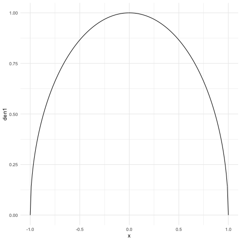
    When ZZ has the semicircle density p(x)(1|x|2)1/2p(x)\propto(1-|x|^{2})^{1/2} (see Figure 3(a)), then 𝔼|Z|γγ32\mathbb{E}|Z|^{\gamma}\propto\gamma^{-\frac{3}{2}} so that θ^γ^\widehat{\theta}_{\widehat{\gamma}} has rate O~(n23)\widetilde{O}(n^{-\frac{2}{3}}), where we use the O~()\widetilde{O}(\cdot) notation to indicate that we have ignored polylog terms.

  2. 2.

    When ZUnif[1,1]Z\sim\text{Unif}[-1,1], we have that 𝔼|Z|γ=1γ+1\mathbb{E}|Z|^{\gamma}=\frac{1}{\gamma+1} so that θ^γ^\widehat{\theta}_{\widehat{\gamma}} has rate O~(n1)\widetilde{O}(n^{-1}).

  3. 3.

    More generally, let qq be a symmetric continuous density on \mathbb{R} and let pp be a density that results from truncating qq, that is, p(x)q(x)𝟙{|x|1}p(x)\propto q(x)\mathbbm{1}\{|x|\leq 1\}. If p(1)=p(1)>0p(1)=p(-1)>0, then a1γ𝔼|Z|γa2γ\frac{a_{1}}{\gamma}\leq\mathbb{E}|Z|^{\gamma}\leq\frac{a_{2}}{\gamma} where a1,a2a_{1},a_{2} depend on qq. In particular, if ZZ is a truncated Gaussian, then γ^γ^\widehat{\gamma}_{\widehat{\gamma}} also has O~(n1)\widetilde{O}(n^{-1}) rate.

  4. 4.

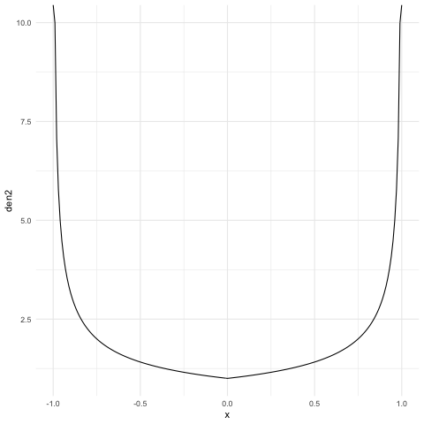
    Suppose ZZ has a U-shaped density of the form p(x)(1|x|)12p(x)\propto(1-|x|)^{-\frac{1}{2}} (Figure 3(b)), then 𝔼|Z|γγ12\mathbb{E}|Z|^{\gamma}\propto\gamma^{-\frac{1}{2}} so that θ^γ^\widehat{\theta}_{\widehat{\gamma}} has rate O~(n2)\widetilde{O}(n^{-2}).

Refer to caption
(a) Semicircle density
Refer to caption
(b) U-shaped density
Figure 3:
Remark 3.2.

By Proposition 6 and the subsequent Remark S2.1 in Section S2.2 of the Appendix, we have that if a density pp is of the form p(x)=Cα(1|x|)α1𝟙{|x|1}p(x)=C_{\alpha}(1-|x|)^{\alpha-1}\mathbbm{1}\{|x|\leq 1\} for α(0,2)\alpha\in(0,2), then we have that, writing H2(θ1,θ2):=(p(xθ1)p(xθ2))2𝑑xH^{2}(\theta_{1},\theta_{2}):=\int\bigl{(}\sqrt{p(x-\theta_{1})}-\sqrt{p(x-\theta_{2})}\bigr{)}^{2}dx,

Cα,1|θ1θ2|αH2(θ1,θ2)Cα,2|θ1θ2|α,C_{\alpha,1}|\theta_{1}-\theta_{2}|^{\alpha}\leq H^{2}(\theta_{1},\theta_{2})\leq C_{\alpha,2}|\theta_{1}-\theta_{2}|^{\alpha},

for Cα,1C_{\alpha,1} and Cα,2C_{\alpha,2} dependent only on α\alpha. From Le Cam (1973, Proposition 1), any estimator θ^\widehat{\theta} has a rate lower bounded by the fact that H2(θ^,θ0)1nH^{2}(\widehat{\theta},\theta_{0})\gtrsim\frac{1}{n} so that among the class of densities

𝒫a1,a2:={p: symmetric,a1γα|x|γp(x)𝑑xa2γα,γ1, for some α(0,2]},\displaystyle\mathcal{P}_{a_{1},a_{2}}:=\biggl{\{}p\,:\,\text{ symmetric},\,\frac{a_{1}}{\gamma^{\alpha}}\leq\int|x|^{\gamma}p(x)dx\leq\frac{a_{2}}{\gamma^{\alpha}},\text{$\forall\gamma\geq 1$, for some $\alpha\in(0,2]$}\biggr{\}}, (6)

our proposed estimator θ^γ^\widehat{\theta}_{\widehat{\gamma}} has a rate of convergence that is minimax optimal up to poly-log factors.

3.2 Comparison with the MLE

Recall from Remark 2.2 that for θ\theta\in\mathbb{R} and σ,γ>0\sigma,\gamma>0, the generalized Gaussian distribution (also known as the Subbotin distribution) has a density of the form p(x:θ,σ,γ)=12σΓ(1+γ1)exp(|xθσ|γ)p(x:\theta,\sigma,\gamma)=\frac{1}{2\sigma\Gamma(1+\gamma^{-1})}\exp\bigl{(}-\bigl{|}\frac{x-\theta}{\sigma}\bigr{|}^{\gamma}\bigr{)}. We note that the uniform distribution on [σ,σ][-\sigma,\sigma] is a limit point of the generalized Gaussian class where we let γ\gamma\rightarrow\infty.

Using univariate observations Y1,,YnY_{1},\ldots,Y_{n}, we may then compute the MLE of γ\gamma with respect to the generalized Gaussian family:

γ^MLE=argminγminθ,σ1ni=1n|Yiθσ|γ+logσ+logΓ(1+1γ).\displaystyle\widehat{\gamma}_{\text{MLE}}=\operatorname*{arg\,min}_{\gamma}\min_{\theta,\sigma}\frac{1}{n}\sum_{i=1}^{n}\biggl{|}\frac{Y_{i}-\theta}{\sigma}\biggr{|}^{\gamma}+\log\sigma+\log\Gamma\biggl{(}1+\frac{1}{\gamma}\biggr{)}.

For any fixed γ\gamma, we may minimize over θ\theta and σ\sigma to obtain that

γ^MLE=argminγLn(γ),\widehat{\gamma}_{\text{MLE}}=\operatorname*{arg\,min}_{\gamma}L_{n}(\gamma),

where

Ln(γ):=1γlog(minθ1ni=1n|Yiθ|γ)+1+logγγ+logΓ(1+1γ).L_{n}(\gamma):=\frac{1}{\gamma}\log\biggl{(}\min_{\theta}\frac{1}{n}\sum_{i=1}^{n}|Y_{i}-\theta|^{\gamma}\biggr{)}+\frac{1+\log\gamma}{\gamma}+\log\Gamma\biggl{(}1+\frac{1}{\gamma}\biggr{)}.

A natural question then is how good is γ^MLE\widehat{\gamma}_{\text{MLE}} as a selection procedure? Would the resulting location estimator θ^γ^MLE\widehat{\theta}_{\widehat{\gamma}_{\text{MLE}}} have good properties? If the density of YiY_{i} belongs to the generalized Gaussian class, then we expect γ^MLE\widehat{\gamma}_{\text{MLE}} to perform well. But when there is model misspecification, we show in this section that γ^MLE\widehat{\gamma}_{\text{MLE}} performs suboptimally compared to the CAVS estimator that we propose in Section 2.3.

To start, let us define the population level likelihood function for every γ>0\gamma>0

L(γ)\displaystyle L(\gamma) :=minθ,σ𝔼|Yθσ|γ+log(2σ)+logΓ(1+1γ)\displaystyle:=\min_{\theta,\sigma}\mathbb{E}\biggl{|}\frac{Y-\theta}{\sigma}\biggr{|}^{\gamma}+\log(2\sigma)+\log\Gamma\bigl{(}1+\frac{1}{\gamma}\bigr{)}
=1γlog(minθ𝔼|Yθ|γ)+1+logγγ+logΓ(1+1γ).\displaystyle=\frac{1}{\gamma}\log\bigl{(}\min_{\theta}\mathbb{E}|Y-\theta|^{\gamma}\bigr{)}+\frac{1+\log\gamma}{\gamma}+\log\Gamma\biggl{(}1+\frac{1}{\gamma}\biggr{)}.

We define L():=limγL(γ)L(\infty):=\lim_{\gamma\rightarrow\infty}L(\gamma) and Ln():=limγLn(γ)=log{(Y(n)Y(1))/2}L_{n}(\infty):=\lim_{\gamma\rightarrow\infty}L_{n}(\gamma)=\log\bigl{\{}(Y_{(n)}-Y_{(1)})/2\bigr{\}}. We note that if 𝔼|Y|γ=\mathbb{E}|Y|^{\gamma}=\infty, then L(γ)=L(\gamma)=\infty and if YY is supported on the real line, then L()=L(\infty)=\infty. Moreover, by Lemma 2 (in Section S1.2 of the appendix), we have that, for any fixed γ{}\gamma\in\mathbb{R}\cup\{\infty\}, we have that Ln(γ)a.s.L(γ)L_{n}(\gamma)\stackrel{{\scriptstyle a.s.}}{{\rightarrow}}L(\gamma).

Define γMLE=argminγ2L(γ)\gamma_{\text{MLE}}^{*}=\operatorname*{arg\,min}_{\gamma\geq 2}L(\gamma) as the minimizer of L(γ)L(\gamma). We show in the next Proposition that when the noise ZiZ_{i} is supported on [1,1][-1,1] with a small but positive density value at the boundary, then γMLE<\gamma_{\text{MLE}}^{*}<\infty even though the optimal selection of γ\gamma is to take γ\gamma\rightarrow\infty since the sample midrange θ^\widehat{\theta}_{\infty} would have a rate of convergence that is at least as fast as O~(n1)\widetilde{O}(n^{-1}).

Proposition 2.

Suppose Y=Z+θ0Y=Z+\theta_{0} where ZZ has a distribution symmetric around 0. Define γMLE=argminγ>0L(γ)\gamma^{*}_{\text{MLE}}=\operatorname*{arg\,min}_{\gamma>0}L(\gamma).

  1. 1.

    If ZZ is supported on all of \mathbb{R}, then γMLE<\gamma^{*}_{\text{MLE}}<\infty.

  2. 2.

    Suppose ZZ has a density pp supported and continuous on [1,1][-1,1]. Let γE0.57721\gamma_{\text{E}}\approx 0.57721 be the Euler–Mascheroni constant. If the density value at the boundary satisfies p(1)<12eγE1p(1)<\frac{1}{2}e^{\gamma_{\text{E}}-1}, then γMLE<\gamma^{*}_{\text{MLE}}<\infty.

  3. 3.

    Suppose ZZ has a density pp supported and continuous on [1,1][-1,1]. If the density value at the boundary satisfies p(1)>12eγE1p(1)>\frac{1}{2}e^{\gamma_{\text{E}}-1}, then γ=\gamma=\infty is a local minimum of L(γ)L(\gamma).

We relegate the proof of Proposition 2 to Section S2.3 of the Appendix.

If the noise density pp is continuous and has boundary value p(1)(0,12eγE1)p(1)\in(0,\frac{1}{2}e^{\gamma_{\text{E}}-1}), then Proposition 2 suggests that we would not expect γ^MLE\widehat{\gamma}_{\text{MLE}}\rightarrow\infty. More precisely, we have that L(γMLE)<L()L(\gamma^{*}_{\text{MLE}})<L(\infty) and thus, by Lemma 2, when nn is large enough, we also have Ln(γMLE)<Ln()L_{n}(\gamma^{*}_{\text{MLE}})<L_{n}(\infty) almost surely. Therefore, selecting γ\gamma by minimizing LnL_{n} would always favor a finite γ=γMLE\gamma=\gamma^{*}_{\text{MLE}} over γ=\gamma=\infty. As a result, selecting γ\gamma based on MLE yields a suboptimal rate of n1/2n^{-1/2}.

In contrast, Theorem 3.1 shows that under the same setting, our proposed CAVS estimator selects a divergent γ^\widehat{\gamma} which can yield an error that is smaller than O~(n1/2)\widetilde{O}(n^{-1/2}) for θ^γ^\widehat{\theta}_{\widehat{\gamma}}. In fact, there are settings in which the density at the boundary is equal to zero, that is, p(1)=0p(1)=0, where our proposed estimator can θ^γ^\widehat{\theta}_{\widehat{\gamma}} have a rate of convergence that is faster than n1/2n^{-1/2}; for example, we see in that |θ^γ^θ0||\widehat{\theta}_{\widehat{\gamma}}-\theta_{0}| is O~(n2/3)\widetilde{O}(n^{-2/3}) when the noise has the semicircle density.

We note that although Proposition 2 is stated for ZZ supported on [1,1][-1,1], by scale invariance of γMLE\gamma^{*}_{\text{MLE}}, Proposition 2 holds for support of the form [b,b][-b,b], where the the condition on the density generalizes to p(b)>12beγ01p(b)>\frac{1}{2b}e^{\gamma_{0}-1}.

Remark 3.3.

Another drawback, one that is perhaps more alarming, of selecting γ\gamma based on the Generalized Gaussian likelihood is that the resulting location estimator may have a standard deviation (and hence error) that is larger than O(n1/2)O(n^{-1/2}).

Consider the following example: let p1p_{1} be the density of |W|13sign(W)|W|^{\frac{1}{3}}\text{sign}(W), where WW follows the standard Cauchy distribution, let p2(x)exp(|x|3)p_{2}(x)\propto\exp\bigl{(}-|x|^{3}\bigr{)}, and let the noise ZZ have a mixture density p=δp1+(1δ)p2p=\delta p_{1}+(1-\delta)p_{2} for some δ[0,1]\delta\in[0,1]. We let Y=Z+θ0Y=Z+\theta_{0} as usual.

If δ=0\delta=0 so that Zp2Z\sim p_{2}, then L(γ)L(\gamma) is minimized at γ=3\gamma=3. It also holds, when δ\delta is sufficiently small (see Lemma 8), the likelihood L(γ)L(\gamma) is also minimized at γ=3\gamma=3 so that the likelihood based selector would likely output θ^3\widehat{\theta}_{3}. However, for any δ>0\delta>0, we have that V(3)V(3), the asymptotic variance of θ^3\widehat{\theta}_{3}, is 𝔼|Z|4(2𝔼|Z|2)=\frac{\mathbb{E}|Z|^{4}}{(2\mathbb{E}|Z|^{2})}=\infty. In contrast, our proposed procedure would output the sample mean Y¯=θ^2\bar{Y}=\widehat{\theta}_{2}, which has finite asymptotic variance. Intuitively, the CAVS procedure behaves better because it takes into account the higher moment 𝔼|Z|2(γ1)\mathbb{E}|Z|^{2(\gamma-1)} whereas the likelihood selector is based only on 𝔼|Z|γ\mathbb{E}|Z|^{\gamma}.

4 Empirical studies

We perform empirical studies on simulated data to verify our theoretical results in Section 3. We also analyze a dataset of NBA player statistics for the 2020-2021 season to show that our proposed CAVS estimator can be directly applied to real data.

4.1 Simulations
Refer to caption
(a) Location estimation
Refer to caption
(b) Regression
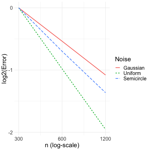
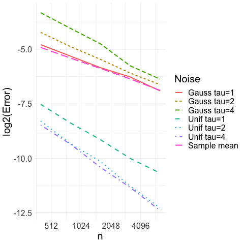
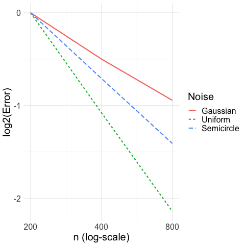
Figure 4: Log-error vs. sample size plots. Sample size nn is plotted on a log-scale.

Convergence rate for location estimation: Our first simulation takes the location estimation setting where Yi=θ0+ZiY_{i}=\theta_{0}+Z_{i} for i=1,,ni=1,\ldots,n. We let the distribution of the noise ZiZ_{i} be either Gaussian N(0,1)N(0,1), uniform Unif[1,1]\text{Unif}[-1,1], or semicircle (see Example 2). We let the sample size nn vary between (200,400,800)(200,400,800). We compute our proposed CAVS estimator θ^γ^\widehat{\theta}_{\widehat{\gamma}} (with τ=log4n200\tau=\sqrt{\log\frac{4n}{200}}) and plot, in Figure 4(a), log-error versus the sample size nn, where nn is plotted on a logarithmic scale. Hence, a rate of convergence of ntn^{-t} would yield an error line of slope t-t in Figure 4(a). We normalize the errors so that all the lines have the same intercept. We see that error under uniform noise has a slope of 1-1, error under semicircle noise has a slope of 2/3-2/3, and error under Gaussian noise has a slope of 1/2-1/2 exactly as predicted by Theorem 2.1 and Theorem 3.1.

Convergence rate for regression: Then, we study the regression setting where Yi=Xiβ0+ZiY_{i}=X_{i}^{\top}\beta_{0}+Z_{i} for i=1,2,,ni=1,2,\ldots,n. We let the distribution of the noise ZiZ_{i} be either Gaussian N(0,1)N(0,1), uniform Unif[1,1]\text{Unif}[-1,1], or the semicircle density given in Example 2. We let the sample size nn vary between (200,400,600)(200,400,600). We apply the regression version of the CAVS estimate β^γ^\widehat{\beta}_{\widehat{\gamma}} as described in Remark 2.5 (with τ=log4n200\tau=\sqrt{\log\frac{4n}{200}}), and plot, in Figure 4(a), log-error versus the sample size nn, where nn is plotted on a logarithmic scale. We see that CAVS also has adaptive rate of convergence; the uniform noise yields a rate of n1n^{-1}, the semicircle noise yields a rate of n2/3n^{-2/3}, and the Gaussian noise yields a rate of n1/2n^{-1/2} as nn increases, as predicted by our theory.
Refer to caption
(a) Gaussian truncated at different levels
Refer to caption
(b) Different τ\tau
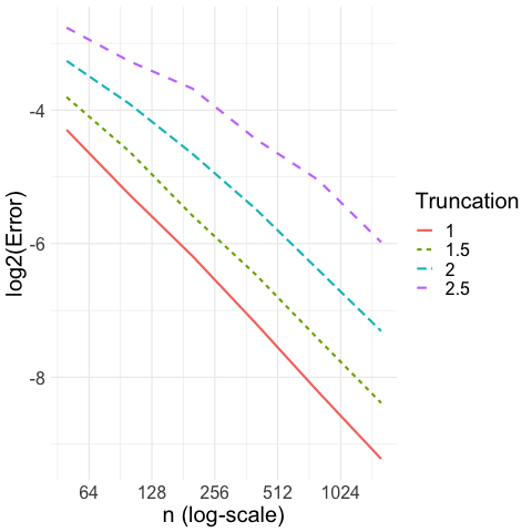
Figure 5: Log-error vs. sample size plots. Sample size nn is plotted on a log-scale.

Convergence rate for truncated Gaussian at different truncation levels: In Figure 5(a), we take the location model Yi=θ0+ZiY_{i}=\theta_{0}+Z_{i} where ZiZ_{i} has the density pt(x)exp{12x2σt2}𝟙(|x|t/σt)p_{t}(x)\propto\exp\{-\frac{1}{2}\frac{x^{2}}{\sigma^{2}_{t}}\}\mathbbm{1}(|x|\leq t/\sigma_{t}) for some t>0t>0 and where σt>0\sigma_{t}>0 is chosen so that ZiZ_{i} always has unit variance. In other words, we sample ZiZ_{i} by first generating WN(0,1)W\sim N(0,1), keep WW only if |W|t|W|\leq t, and then take Zi=σtWZ_{i}=\sigma_{t}W where σt>0\sigma_{t}>0 is chosen so that Var(Zi)=1\text{Var}(Z_{i})=1. We use four different truncation levels t=1,1.5,2,2.5t=1,1.5,2,2.5; we let the sample size vary from n=50n=50 to n=1600n=1600 and compute our CAVS estimate θ^γ^\widehat{\theta}_{\widehat{\gamma}} (with τ=log4n50\tau=\sqrt{\log\frac{4n}{50}}). We plot in Figure 5(a), the log-error versus the sample size nn, where nn is plotted on a logarithmic scale. We observe that when the truncation level is t=1t=1 or 1.51.5 or 22, the error is of order n1n^{-1}. When the truncation level is t=2.5t=2.5, the error behaves like n1/2n^{-1/2} for small nn but transitions to n1n^{-1} when nn becomes large. This is not surprising since, when nn is small, it is difficult to know whether the ZiZ_{i}’s are drawn from N(0,1)N(0,1) or drawn from truncated Gaussian with a large truncation level.

Convergence rate for different τ\tau: In Figure 5(b), we take the location model Yi=θ0+ZiY_{i}=\theta_{0}+Z_{i} and take ZiZ_{i} to be either Gaussian N(0,1)N(0,1) or uniform Unif[M,M]\text{Unif}[-M,M] where M>0M>0 is chosen so that ZiZ_{i} has unit variance. We then apply our proposed CAVS procedure for different levels of τ\tau, ranging from τ{1,2,4}\tau\in\{1,2,4\}. We let the sample size vary from n=400n=400 to n=6400n=6400 and plot the log-error versus the sample size nn, where nn is plotted on a logarithmic scale. For comparison, we also plot the error of the sample mean Y¯\bar{Y}, which does not depend on the distribution of ZiZ_{i} since we scale ZiZ_{i} to have unit variance in both settings. We observe in Figure 5(b) that when τ=1\tau=1, the CAVS estimate θ^γ^\widehat{\theta}_{\widehat{\gamma}} basically coincides with the sample mean if ZiN(0,1)Z_{i}\sim N(0,1) but has much less error when ZiZ_{i} is uniform. As we increase τ\tau, CAVS estimator has increased error under the Gaussian setting when ZiN(0,1)Z_{i}\sim N(0,1) since we select γ^>2\widehat{\gamma}>2 more often; under the uniform setting, it has less error. Based on these studies, we recommend τ=1\tau=1 in practice as a conservative choice.

4.2 Real data experiments

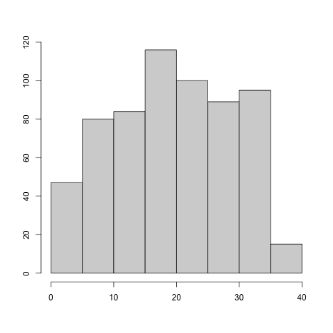
Uniform or truncated Gaussian data are not ubiquitous but they do appear in real world datasets. In this section, we use the CAVS location estimation and regression procedure to analyze a dataset of 626 NBA players in the 2020–2021 season. We consider variables AGE, MPG (average minutes played per game), and GP (games played).
Refer to caption
(a) Histogram of MPG
Refer to caption
(b) V^(γ)\widehat{V}(\gamma)
Refer to caption
(c) θ^γ±V^(γ)n\widehat{\theta}_{\gamma}\pm\sqrt{\frac{\widehat{V}(\gamma)}{n}}
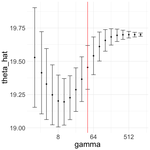
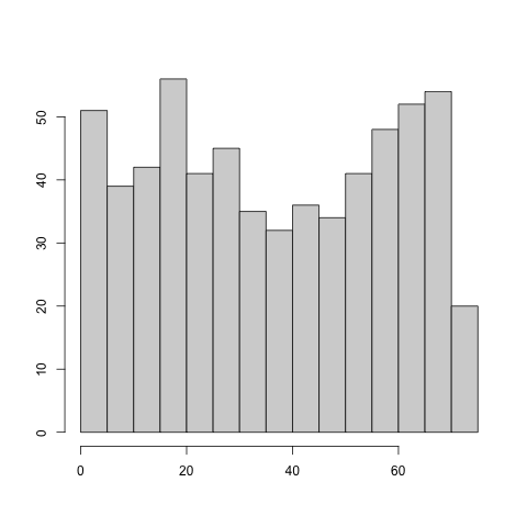
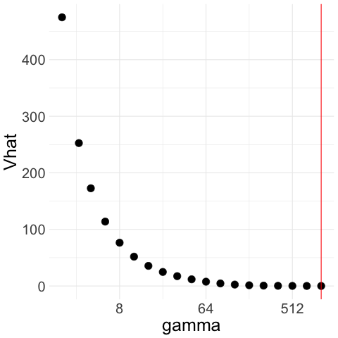
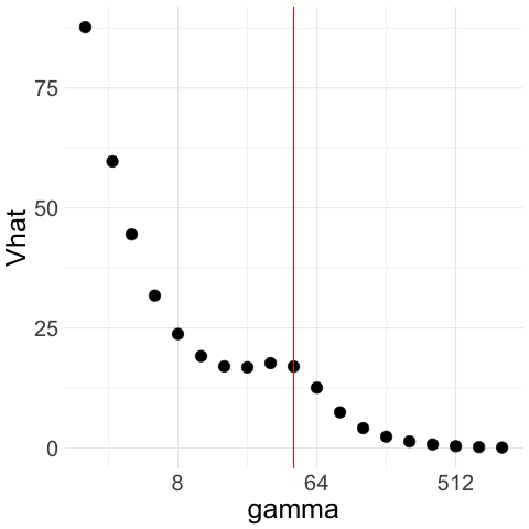
Figure 6: Analysis on MPG (average minutes played per game) in the NBA 2021 data

Both MPG and GP variables are compactly supported. They also do not exhibit clear signs of asymmetry; MPG has an empirical skewness of 0.064-0.064 and GP has an empirical skewness of 0.0130.013. We apply the CAVS procedure to both with τ=1\tau=1 and we obtain γ^=32\widehat{\gamma}=32 for MPG variable and γ^=2048\widehat{\gamma}=2048 for the GP variable. In contrast, the AGE variable has a skewness of 0.560.56 and when we apply CAVS procedure (still with τ=1\tau=1), we obtain γ^=2\widehat{\gamma}=2. These results suggest that CAVS can be useful for practical data analysis.

Moreover, we also study the CAVS regression method by considering two regression models:

(MODEL 1)MPGGP+AGE+W,(MODEL 2)MPGAGE+W,(\text{MODEL 1})\,\,\text{MPG}\sim\text{GP}+\text{AGE}+\text{W},\qquad(\text{MODEL 2})\,\,\text{MPG}\sim\text{AGE}+\text{W},

where W is an independent Gaussian feature add so that we can assess how close the estimated coefficient β^W\widehat{\beta}_{\text{W}} is to zero to gauge the estimation error. We estimate β^γ^\widehat{\beta}_{\widehat{\gamma}} on 100 randomly chosen training data points and report the predictive error on the remaining test data points; we also report the average value of |β^W||\widehat{\beta}_{\text{W}}|, which we would like to be as close to 0 as possible. We perform 1000 trials of this experiment (choosing random training set in each trial) and report the performance of CAVS versus OLS estimator in Table 1.

Model 1 Pred. Error Model 1 |β^W||\widehat{\beta}_{\text{W}}| Model 2 Pred. Error Model 2 |β^W||\widehat{\beta}_{\text{W}}|
CAVS 0.686 0.045 0.95 0.082
OLS 0.689 0.140 1.04 0.205
Table 1: Comparison of CAVS vs. OLS on two simple regression models.
Refer to caption
(a) Histogram of GP
Refer to caption
(b) V^(γ)\widehat{V}(\gamma)
Refer to caption
(c) θ^γ±V^(γ)n\widehat{\theta}_{\gamma}\pm\sqrt{\frac{\widehat{V}(\gamma)}{n}}
Figure 7: Analysis on GP (games played) in the NBA 2021 data

5 Discussion

In this paper, we give an estimator of the location of a symmetric distribution whose rate of convergence can be faster than the usual n\sqrt{n} and can adapt to the unknown underlying density. There are a number of interesting open questions that remain:

  • It is unclear whether the excess log-factors in our adaptive rate result is an artifact of the analysis or an unavoidable cost of adaptivity.

  • We emphasize that it is the discontinuity of the noise density pp (or the singularities of the derivative pp^{\prime}) on the boundary of the support [1,1][-1,1] that allows our estimator to have rates of convergence faster than 1/n1/\sqrt{n}. Any discontinuities of the noise density (or the singularities of the density derivative) in the interior of the support will also lead to an infinite Fisher information (for the location parameter) and open the possibility of faster-than-root-n rate. Our estimator unfortunately cannot adapt to discontinuities in the interior. For example, if the noise density is a mixture of Uniform[1,1][-1,1] and Gaussian N(0,1)N(0,1), the tail of the Gaussian component would imply that our estimator cannot have a rate faster than root-n. On the other hand, an oracle with knowledge of the discontinuity points at ±1\pm 1 could still estimate θ0\theta_{0} at n1n^{-1} rate with the estimator argmaxθ1ni=1n𝟙{Yi[θ1,θ+1]}\operatorname*{arg\,max}_{\theta}\frac{1}{n}\sum_{i=1}^{n}\mathbbm{1}\{Y_{i}\in[\theta-1,\theta+1]\}. One potential approach for adapting to discontinuities in the interior is to first estimate the position of these discontinuity points. However, the position must be estimated with a high degree of accuracy as any error would percolate to the down-stream location estimator. We leave a formal investigation of this line of inquiry to future work.

  • It would be nontrivial to extend our rate adaptivity result to the multivariate setting, for instance, if Yi=θ0+ZiY_{i}=\theta_{0}+Z_{i} where θ0d\theta_{0}\in\mathbb{R}^{d} and ZiZ_{i} is uniformly distributed on a convex body KdK\subset\mathbb{R}^{d} that is balanced in that K=KK=-K so that Zi=dZiZ_{i}\stackrel{{\scriptstyle d}}{{=}}-Z_{i}. When KK is known, it would be natural to study estimators of the form θ^γ=argminθdi=1nYiθKγ\widehat{\theta}_{\gamma}=\operatorname*{arg\,min}_{\theta\in\mathbb{R}^{d}}\sum_{i=1}^{n}\|Y_{i}-\theta\|_{K}^{\gamma} where K\|\cdot\|_{K} is the gauge function (Minkowski functional) associated with KK. In general, it would be necessary to simultaneously estimate KK and θ0\theta_{0}. Xu and Samworth (2021) studies an approach where one first estimates θ0\theta_{0} via the sample mean and then compute K^\widehat{K} using the convex hull of the directional quantiles of the data. This however cannot achieve a rate faster than root-n.

  • When applied in the linear regression setting, our CAVS procedure performs well empirically on both synthetic and real data. It would thus be interesting to rigorously establish a rate adaptivity result in the linear regression model. More generally, in a nonparametric regression model Yi=f(Xi)+ZiY_{i}=f(X_{i})+Z_{i} where the noise ZiZ_{i} has a noise distribution symmetric around 0 and the regression function ff lies in some nonparametric function class \mathcal{F}, we can still use our procedure to select amongst estimators of the form f^γ=argminfi=1n|Yif(Xi)|γ\widehat{f}_{\gamma}=\operatorname*{arg\,min}_{f\in\mathcal{F}}\sum_{i=1}^{n}|Y_{i}-f(X_{i})|^{\gamma}. Understanding the statistical properties of this procedure would motivate the use of γ\ell^{\gamma} loss functions, for γ>2\gamma>2, in general regression problems.

Acknowledgement

The first and second authors are supported by NSF grant DMS-2113671. The authors are very grateful to Richard Samworth for suggesting the use of Lepski’s method. The authors further thank Jason Klusowski for many insightful discussions.

References

  • (1)
  • Baraud and Birgé (2018) Baraud, Y. and Birgé, L. (2018). Rho-estimators revisited: General theory and applications, The Annals of Statistics 46(6B): 3767–3804.
  • Baraud et al. (2017) Baraud, Y., Birgé, L. and Sart, M. (2017). A new method for estimation and model selection: ρ\rho-estimation, Inventiones mathematicae 207(2): 425–517.
  • Beran (1978) Beran, R. (1978). An efficient and robust adaptive estimator of location, The Annals of Statistics pp. 292–313.
  • Bickel (1982) Bickel, P. J. (1982). On adaptive estimation, The Annals of Statistics pp. 647–671.
  • Bickel et al. (1993) Bickel, P. J., Klaassen, C. A., Ritov, Y. and Wellner, J. A. (1993). Efficient and adaptive estimation for semiparametric models, Vol. 4, Springer.
  • Bloch and Gastwirth (1968) Bloch, D. A. and Gastwirth, J. L. (1968). On a simple estimate of the reciprocal of the density function, The Annals of Mathematical Statistics 39(3): 1083–1085.
  • Chierichetti et al. (2014) Chierichetti, F., Dasgupta, A., Kumar, R. and Lattanzi, S. (2014). Learning entangled single-sample gaussians, Proceedings of the twenty-fifth annual ACM-SIAM symposium on Discrete algorithms, SIAM, pp. 511–522.
  • Dalalyan et al. (2006) Dalalyan, A., Golubev, G. and Tsybakov, A. (2006). Penalized maximum likelihood and semiparametric second-order efficiency, The Annals of Statistics 34(1): 169–201.
  • Giné and Nickl (2016) Giné, E. and Nickl, R. (2016). Mathematical foundations of infinite-dimensional statistical models, Cambridge university press.
  • Huber (2011) Huber, P. J. (2011). Robust statistics, International encyclopedia of statistical science, Springer, pp. 1248–1251.
  • Ibragimov and Has’ Minskii (2013) Ibragimov, I. A. and Has’ Minskii, R. Z. (2013). Statistical estimation: asymptotic theory, Vol. 16, Springer Science & Business Media.
  • Laha (2021) Laha, N. (2021). Adaptive estimation in symmetric location model under log-concavity constraint, Electronic Journal of Statistics 15(1): 2939–3014.
  • Lai et al. (1983) Lai, T., Robbins, H. and Yu, K. (1983). Adaptive choice of mean or median in estimating the center of a symmetric distribution, Proceedings of the National Academy of Sciences 80(18): 5803–5806.
  • Le Cam (1973) Le Cam, L. (1973). Convergence of estimates under dimensionality restrictions, Annals of Statistics 1(1): 38–53.
  • Lepskii (1990) Lepskii, O. (1990). On a problem of adaptive estimation in gaussian white noise, Theory of Probability & Its Applications 35(3): 454–466.
  • Lepskii (1991) Lepskii, O. (1991). Asymptotically minimax adaptive estimation. i: Upper bounds. optimally adaptive estimates, Theory of Probability & Its Applications 36(4): 682–697.
  • Mammen and Park (1997) Mammen, E. and Park, B. U. (1997). Optimal smoothing in adaptive location estimation, Journal of statistical planning and inference 58(2): 333–348.
  • Pensia et al. (2019) Pensia, A., Jog, V. and Loh, P.-L. (2019). Estimating location parameters in entangled single-sample distributions, arXiv preprint arXiv:1907.03087 .
  • Schick (1986) Schick, A. (1986). On asymptotically efficient estimation in semiparametric models, The Annals of Statistics pp. 1139–1151.
  • Stein (1956) Stein, C. (1956). Efficient nonparametric testing and estimation, Proceedings of the third Berkeley symposium on mathematical statistics and probability, Vol. 1, pp. 187–195.
  • Stone (1975) Stone, C. J. (1975). Adaptive maximum likelihood estimators of a location parameter, The Annals of Statistics pp. 267–284.
  • Subbotin (1923) Subbotin, M. T. (1923). On the law of frequency of error, Matematicheskii Sbornik 31(2): 296–301.
  • Van Der Vaart and Wellner (1996) Van Der Vaart, A. W. and Wellner, J. (1996). Weak convergence and empirical processes: with applications to statistics, Springer Science & Business Media.
  • Van Der Vaart and Wellner (2011) Van Der Vaart, A. and Wellner, J. A. (2011). A local maximal inequality under uniform entropy, Electronic Journal of Statistics 5(2011): 192.
  • Van Eeden (1970) Van Eeden, C. (1970). Efficiency-robust estimation of location, The Annals of Mathematical Statistics 41(1): 172–181.
  • Xu and Samworth (2021) Xu, M. and Samworth, R. J. (2021). High-dimensional nonparametric density estimation via symmetry and shape constraints, The Annals of Statistics 49(2): 650–672.

Supplementary material to “Rate optimal and adaptive estimation of the center of a symmetric distribution”

Yu-Chun Kao, Min Xu, and Cun-Hui Zhang

S1 Supplementary material for Section 2

S1.1 Proof of Lemma 1

Proof.

(of Lemma 1)

First, we observe that if 4lognγ14\frac{\log n}{\gamma}\geq 1, then, by the fact that θ^γ[X(1),X(n)]\widehat{\theta}_{\gamma}\in[X_{(1)},X_{(n)}], we have that

|θ^γXmid|12(X(n)X(1))2(X(n)X(1))lognγ.|\widehat{\theta}_{\gamma}-X_{\text{mid}}|\leq\frac{1}{2}(X_{(n)}-X_{(1)})\leq 2(X_{(n)}-X_{(1)})\frac{\log n}{\gamma}.

Therefore, we assume that 4lognγ14\frac{\log n}{\gamma}\leq 1.

We apply Lemma 3 with f(θ)={1ni=1n|Xiθ|γ}1/γf(\theta)=\bigl{\{}\frac{1}{n}\sum_{i=1}^{n}|X_{i}-\theta|^{\gamma}\bigr{\}}^{1/\gamma} and g(θ)=maxi|Xiθ|g(\theta)=\max_{i}|X_{i}-\theta| so that θg:=argming(θ)=θ^mid\theta_{g}:=\operatorname*{arg\,min}g(\theta)=\widehat{\theta}_{\text{mid}} and θf:=argminf(θ)=θ^γ\theta_{f}:=\operatorname*{arg\,min}f(\theta)=\widehat{\theta}_{\gamma}. Fix any δ>0\delta>0. We observe that

g(θg)\displaystyle g(\theta_{g}) =maxi|XiXmid|=X(n)X(1)2\displaystyle=\max_{i}|X_{i}-X_{\text{mid}}|=\frac{X_{(n)}-X_{(1)}}{2}
g(θg+δ)\displaystyle g(\theta_{g}+\delta) =X(n)X(1)2+δ, and g(θgδ)=X(n)X(1)2+δ.\displaystyle=\frac{X_{(n)}-X_{(1)}}{2}+\delta,\qquad\text{ and }g(\theta_{g}-\delta)=\frac{X_{(n)}-X_{(1)}}{2}+\delta.

Therefore, for θ{θgδ,θg+δ}\theta\in\{\theta_{g}-\delta,\theta_{g}+\delta\}, we have that 12(g(θ)g(θg))=δ2\frac{1}{2}(g(\theta)-g(\theta_{g}))=\frac{\delta}{2}. On the other hand, by the fact that

{1ni=1n|Xiθ|γ}1γn1γmaxi[n]|Xiθ|,\biggl{\{}\frac{1}{n}\sum_{i=1}^{n}|X_{i}-\theta|^{\gamma}\biggr{\}}^{\frac{1}{\gamma}}\geq n^{-\frac{1}{\gamma}}\max_{i\in[n]}|X_{i}-\theta|,

we have that

g(θ)f(θ)n1γg(θ)θ.\displaystyle g(\theta)\geq f(\theta)\geq n^{-\frac{1}{\gamma}}g(\theta)\quad\forall\theta\in\mathbb{R}. (S1.1)

Therefore, for θ{θgδ,θg,θg+δ}\theta\in\{\theta_{g}-\delta,\theta_{g},\theta_{g}+\delta\}, we have that

|f(θ)g(θ)|\displaystyle|f(\theta)-g(\theta)| =g(θ)f(θ)(1n1γ)g(θ)\displaystyle=g(\theta)-f(\theta)\leq(1-n^{-\frac{1}{\gamma}})g(\theta)
lognγ(X(n)X(1)2+δ).\displaystyle\leq\frac{\log n}{\gamma}\biggl{(}\frac{X_{(n)}-X_{(1)}}{2}+\delta\biggr{)}.

Using our assumption that 4lognγ14\frac{\log n}{\gamma}\leq 1, we have that for any δ2(X(n)X(1))lognγ\delta\geq 2(X_{(n)}-X_{(1)})\frac{\log n}{\gamma} and any θ{θgδ,θg,θg+δ}\theta\in\{\theta_{g}-\delta,\theta_{g},\theta_{g}+\delta\},

|f(θ)g(θ)|lognγ(X(n)X(1)2+δ)δ2=12(g(θ)g(θg)).|f(\theta)-g(\theta)|\leq\frac{\log n}{\gamma}\biggl{(}\frac{X_{(n)}-X_{(1)}}{2}+\delta\biggr{)}\leq\frac{\delta}{2}=\frac{1}{2}(g(\theta)-g(\theta_{g})).

The Lemma thus immediately follows from Lemma 3. ∎

S1.2 Lemma 2 on the convergence of V^(γ)\widehat{V}(\gamma)

The following lemma implies that, for a fixed γ\gamma such that V(γ)V(\gamma) is well-defined, our asymptotic variance estimator V^(γ)\widehat{V}(\gamma) is consistent. For a random variable YY, we define its essential supremum to be

ess-sup(Y):=inf{M:(YM)=1},\text{ess-sup}(Y):=\inf\bigl{\{}M\in\mathbb{R}\,:\,\mathbb{P}(Y\leq M)=1\bigr{\}},

where the infimum of an empty set is taken to be infinity. Note that ess-sup(|Y|)<\text{ess-sup}(|Y|)<\infty if and only if YY is compacted supported and that limγ{𝔼|Y|γ}1γ=ess-sup(|Y|)\lim_{\gamma\rightarrow\infty}\{\mathbb{E}|Y|^{\gamma}\}^{\frac{1}{\gamma}}=\text{ess-sup}(|Y|).

We may define ess-inf(Y)\text{ess-inf}(Y) is the same way. For an infinite sequence Y1,Y2,Y_{1},Y_{2},\ldots of independent and identically distributed random variables, it is straightforward to show that Y(n),n:=maxi[n]Yia.s.ess-sup(Y)Y_{(n),n}:=\max_{i\in[n]}Y_{i}\stackrel{{\scriptstyle\text{a.s.}}}{{\rightarrow}}\text{ess-sup}(Y) and Y(1),n:=mini[n]Yia.s.ess-inf(Y)Y_{(1),n}:=\min_{i\in[n]}Y_{i}\stackrel{{\scriptstyle\text{a.s.}}}{{\rightarrow}}\text{ess-inf}(Y) regardless of whether the essential supremum and infimum are finite or not.

Lemma 2.

Let Y1,Y2,Y_{1},Y_{2},\ldots be a sequence of independent and identically distributed random variables and let γ>1\gamma>1. The following hold:

  1. 1.

    If 𝔼|Y|γ<\mathbb{E}|Y|^{\gamma}<\infty, then minθ1ni=1n|Yiθ|γa.s.minθ𝔼|Yθ|γ\min_{\theta\in\mathbb{R}}\frac{1}{n}\sum_{i=1}^{n}|Y_{i}-\theta|^{\gamma}\stackrel{{\scriptstyle a.s.}}{{\rightarrow}}\min_{\theta\in\mathbb{R}}\mathbb{E}|Y-\theta|^{\gamma}.

  2. 2.

    If 𝔼|Y|γ=\mathbb{E}|Y|^{\gamma}=\infty, then minθ1ni=1n|Yiθ|γa.s.\min_{\theta\in\mathbb{R}}\frac{1}{n}\sum_{i=1}^{n}|Y_{i}-\theta|^{\gamma}\stackrel{{\scriptstyle a.s.}}{{\rightarrow}}\infty.

  3. 3.

    If YY is compactly supported, then we have that minθmaxin|Yiθ|=(Y(n),nY(1),n)/2a.s.minθess-sup(|Yθ|)\min_{\theta\in\mathbb{R}}\max_{i\leq n}|Y_{i}-\theta|=(Y_{(n),n}-Y_{(1),n})/2\stackrel{{\scriptstyle a.s.}}{{\rightarrow}}\min_{\theta}\text{ess-sup}(|Y-\theta|).

  4. 4.

    If ess-sup(|Y|)=\text{ess-sup}(|Y|)=\infty, then minθmaxin|Yiθ|a.s.\min_{\theta\in\mathbb{R}}\max_{i\leq n}|Y_{i}-\theta|\stackrel{{\scriptstyle a.s.}}{{\rightarrow}}\infty.

As a direct consequence, for any γ>1\gamma>1 such that 𝔼|Y|γ2<\mathbb{E}|Y|^{\gamma-2}<\infty, we have V^(γ)a.s.V(γ)\widehat{V}(\gamma)\stackrel{{\scriptstyle a.s.}}{{\rightarrow}}V(\gamma), even when V(γ)=V(\gamma)=\infty.

Proof.

(of Lemma 2)

For the first claim, we apply Proposition 3 with g(y,θ)=|yθ|γg(y,\theta)=|y-\theta|^{\gamma} and ψ(θ)=𝔼|Yθ|γ\psi(\theta)=\mathbb{E}|Y-\theta|^{\gamma} and immediately obtain the desired conclusion.

We now prove the second claim by a truncation argument. Suppose 𝔼|Y|γ=\mathbb{E}|Y|^{\gamma}=\infty so that minθ𝔼|Yθ|γ=\min_{\theta}\mathbb{E}|Y-\theta|^{\gamma}=\infty. Fix M>0M>0 arbitrarily. We claim there then exists τ>0\tau>0 such that

minθ𝔼[|Yθ|γ𝟙{|Y|τ}]>M.\min_{\theta\in\mathbb{R}}\mathbb{E}\bigl{[}|Y-\theta|^{\gamma}\mathbbm{1}\{|Y|\leq\tau\}\bigr{]}>M.

To see this, for any τ>0\tau>0, define θτ=argminθ𝔼[|Yθ|γ𝟙{|Y|τ}]\theta_{\tau}=\operatorname*{arg\,min}_{\theta\in\mathbb{R}}\mathbb{E}\bigl{[}|Y-\theta|^{\gamma}\mathbbm{1}\{|Y|\leq\tau\}\bigr{]}. The argmin is well-defined since θ𝔼[|Yθ|γ𝟙{|Y|τ}]\theta\mapsto\mathbb{E}\bigl{[}|Y-\theta|^{\gamma}\mathbbm{1}\{|Y|\leq\tau\}\bigr{]} is strongly convex and goes to infinity as |θ||\theta|\rightarrow\infty. If {θτ}τ=1\{\theta_{\tau}\}_{\tau=1}^{\infty} is bounded, then the claim follows because 𝔼|Yθτ|γ𝟙{|Y|τ}{(𝔼|Y|γ𝟙{|Y|τ})1/γθτ}γ\mathbb{E}|Y-\theta_{\tau}|^{\gamma}\mathbbm{1}\{|Y|\leq\tau\}\geq\{(\mathbb{E}|Y|^{\gamma}\mathbbm{1}\{|Y|\leq\tau\})^{1/\gamma}-\theta_{\tau}\}^{\gamma}. If {θτ}τ=1\{\theta_{\tau}\}_{\tau=1}^{\infty} is unbounded, then there exists a sub-sequence τm\tau_{m} such that limmθτm\lim_{m\rightarrow\infty}\theta_{\tau_{m}}\rightarrow\infty say. For any a>0a>0 such that (|Y|a)>0\mathbb{P}(|Y|\leq a)>0, we have limm𝔼|Yθτm|γ𝟙{|Y|τm}limm|aθτm|γ(|Y|a)=\lim_{m\rightarrow\infty}\mathbb{E}|Y-\theta_{\tau_{m}}|^{\gamma}\mathbbm{1}\{|Y|\leq\tau_{m}\}\geq\lim_{m\rightarrow\infty}|a-\theta_{\tau_{m}}|^{\gamma}\mathbb{P}(|Y|\leq a)=\infty. Therefore, in either cases, our claim holds.

Using Proposition 3 again with g(x,θ)=|xθ|γ𝟙{|x|τ}g(x,\theta)=|x-\theta|^{\gamma}\mathbbm{1}\{|x|\leq\tau\}, we have that

minθ1ni=1n|Yiθ|γ𝟙{|Yi|τ}a.s.minθ𝔼[|Yθ|γ𝟙{|Y|τ}]>M.\min_{\theta}\frac{1}{n}\sum_{i=1}^{n}|Y_{i}-\theta|^{\gamma}\mathbbm{1}\{|Y_{i}|\leq\tau\}\stackrel{{\scriptstyle a.s.}}{{\rightarrow}}\min_{\theta}\mathbb{E}\bigl{[}|Y-\theta|^{\gamma}\mathbbm{1}\{|Y|\leq\tau\}\bigr{]}>M.

In other words, there exists an event Ω~M\widetilde{\Omega}_{M} with probability 1 such that, for any ωΩ~M\omega\in\widetilde{\Omega}_{M}, there exists nωn_{\omega} such that for all nnωn\geq n_{\omega},

minθ1ni=1n|Yiθ|γ\displaystyle\min_{\theta}\frac{1}{n}\sum_{i=1}^{n}|Y_{i}-\theta|^{\gamma} minθ1ni=1n|Yiθ|γ𝟙{|Yi|τ}M/2.\displaystyle\geq\min_{\theta}\frac{1}{n}\sum_{i=1}^{n}|Y_{i}-\theta|^{\gamma}\mathbbm{1}\{|Y_{i}|\leq\tau\}\geq M/2.

Thus, on Ω~M\widetilde{\Omega}_{M}, we have that

lim infnminθ1ni=1n|Yiθ|γ>M/2.\liminf_{n\rightarrow\infty}\min_{\theta}\frac{1}{n}\sum_{i=1}^{n}|Y_{i}-\theta|^{\gamma}>M/2.

Thus, on the event Ω~=M=1Ω~M\widetilde{\Omega}=\cap_{M=1}^{\infty}\widetilde{\Omega}_{M}, we have that minθ1ni=1n|Yiθ|γ\min_{\theta}\frac{1}{n}\sum_{i=1}^{n}|Y_{i}-\theta|^{\gamma}\rightarrow\infty. Since Ω~\widetilde{\Omega} has probability 1, the second claim follows. For the third claim, without loss of generality, we can assume that ess-sup(Y)=1\text{ess-sup}(Y)=1 and ess-inf(Y)=1\text{ess-inf}(Y)=-1. Define Xn=(Y(n),nY(1),n)/2X_{n}=(Y_{(n),n}-Y_{(1),n})/2, then we have Xnminθess-sup(|Yθ|)=1X_{n}\leq\min_{\theta}\text{ess-sup}(|Y-\theta|)=1 and

{Xn<1δ}{Y(n),n<1δ}+{Y(1),n>1+δ},\displaystyle\mathbb{P}\{X_{n}<1-\delta\}\leq\mathbb{P}\{Y_{(n),n}<1-\delta\}+\mathbb{P}\{Y_{(1),n}>-1+\delta\},

where, as nn\rightarrow\infty, the right hand side tends to 0 for every δ>0\delta>0. XnX_{n} thus converges to 11 in probability. Since the collection {Xn}n=1\{X_{n}\}_{n=1}^{\infty} is defined on the same infinite sequence {Y1,Y2,}\{Y_{1},Y_{2},\ldots\} of independent and identically distributed random variables, we have that 1XnXn101\geq X_{n}\geq X_{n-1}\geq 0 so that Xna.s.1X_{n}\stackrel{{\scriptstyle a.s.}}{{\rightarrow}}1 by the monotone convergence theorem.

For the forth claim, suppose without loss of generality that ess-inf(Y)1\text{ess-inf}(Y)\leq-1 and that ess-sup(Y)=\text{ess-sup}(Y)=\infty. Let Xn=(Y(n),nY(1),n)/2X_{n}=(Y_{(n),n}-Y_{(1),n})/2 as with the proof of the third claim. Then,

{Xn<M}{Y(n),n<2M}+{Y(1),n0}.\displaystyle\mathbb{P}\{X_{n}<M\}\leq\mathbb{P}\{Y_{(n),n}<2M\}+\mathbb{P}\{Y_{(1),n}\geq 0\}.

Since the right hand side tends to 0 for every M>0M>0, we have that XnX_{n} converges to infinity almost surely. The Lemma follows as desired. ∎

S1.3 Bound on VV

The following lower bound on V(γ)V(\gamma) holds regardless of whether YY is symmetric around θ0\theta_{0} or not. We have

V(γ)\displaystyle V(\gamma) =𝔼|Yθ0|2(γ1)(γ1)2{𝔼|Yθ0|γ2}2\displaystyle=\frac{\mathbb{E}|Y-\theta_{0}|^{2(\gamma-1)}}{(\gamma-1)^{2}\{\mathbb{E}|Y-\theta_{0}|^{\gamma-2}\}^{2}}
=𝔼|Yθ0|2(γ1){𝔼|Yθ0|γ1}2(𝔼|Yθ0|γ1𝔼|Yθ0|γ2)21(γ1)2\displaystyle=\frac{\mathbb{E}|Y-\theta_{0}|^{2(\gamma-1)}}{\{\mathbb{E}|Y-\theta_{0}|^{\gamma-1}\}^{2}}\biggl{(}\frac{\mathbb{E}|Y-\theta_{0}|^{\gamma-1}}{\mathbb{E}|Y-\theta_{0}|^{\gamma-2}}\biggr{)}^{2}\frac{1}{(\gamma-1)^{2}}
𝔼|Yθ0|2(γ1){𝔼|Yθ0|γ1}2{𝔼|Yθ0|γ2}2γ21(γ1)2\displaystyle\geq\frac{\mathbb{E}|Y-\theta_{0}|^{2(\gamma-1)}}{\{\mathbb{E}|Y-\theta_{0}|^{\gamma-1}\}^{2}}\{\mathbb{E}|Y-\theta_{0}|^{\gamma-2}\}^{\frac{2}{\gamma-2}}\frac{1}{(\gamma-1)^{2}}
𝔼|Yθ0|2(γ1){𝔼|Yθ0|γ1}2𝔼|Yθ0|21(γ1)2,\displaystyle\geq\frac{\mathbb{E}|Y-\theta_{0}|^{2(\gamma-1)}}{\{\mathbb{E}|Y-\theta_{0}|^{\gamma-1}\}^{2}}\mathbb{E}|Y-\theta_{0}|^{2}\frac{1}{(\gamma-1)^{2}},

where the first inequality follows from the fact that 𝔼|Yθ0|γ1(𝔼|Yθ0|γ2)γ1γ2\mathbb{E}|Y-\theta_{0}|^{\gamma-1}\geq\bigl{(}\mathbb{E}|Y-\theta_{0}|^{\gamma-2}\bigr{)}^{\frac{\gamma-1}{\gamma-2}}. In particular, we have that V(γ)𝔼|Yθ0|2(γ1)2V(\gamma)\geq\frac{\mathbb{E}|Y-\theta_{0}|^{2}}{(\gamma-1)^{2}}. Equality is attained when Yθ0Y-\theta_{0} is a Rademacher random variable.

S1.4 Optimization algorithm

We give the Newton’s method algorithm for computing θ^γ=argminθ1ni=1n|Yiθ|γ\widehat{\theta}_{\gamma}=\operatorname*{arg\,min}_{\theta\in\mathbb{R}}\frac{1}{n}\sum_{i=1}^{n}|Y_{i}-\theta|^{\gamma}. It is important to note that to avoid numerical precision issues when γ\gamma is large, we have to transform the input Y1,,YnY_{1},\ldots,Y_{n} so that they are supported on the unit interval [1,1][-1,1].

Algorithm 2 Newton’s method for location estimation

INPUT: observations Y1,,YnY_{1},\ldots,Y_{n}\in\mathbb{R} and γ2\gamma\geq 2.

OUTPUT: θ^γ:=minθ1ni=1n|Yiθ|γ\widehat{\theta}_{\gamma}:=\min_{\theta\in\mathbb{R}}\frac{1}{n}\sum_{i=1}^{n}|Y_{i}-\theta|^{\gamma}.

1:Compute S=(Y(n)Y(1))S=(Y_{(n)}-Y_{(1)}) and M=(Y(n)+Y(1))/2M=(Y_{(n)}+Y_{(1)})/2 and transform Yi2(YiM)/SY_{i}\leftarrow 2(Y_{i}-M)/S.
2:Initialize θ(0)=0\theta^{(0)}=0.
3:for t=1,2,3,t=1,2,3,\ldots do
4:  Compute f=1ni=1n|Yiθ(t1)|γ1sign(Yiθ(t1))f^{\prime}=-\frac{1}{n}\sum_{i=1}^{n}|Y_{i}-\theta^{(t-1)}|^{\gamma-1}\text{sign}(Y_{i}-\theta^{(t-1)})
5:  Compute f′′=γ1ni=1n|Yiθ(t1)|γ2f^{\prime\prime}=\frac{\gamma-1}{n}\sum_{i=1}^{n}|Y_{i}-\theta^{(t-1)}|^{\gamma-2}.
6:  Set θ(t)=θ(t1)ff′′\theta^{(t)}=\theta^{(t-1)}-\frac{f^{\prime}}{f^{\prime\prime}}.
7:  If |f|ε|f^{\prime}|\leq\varepsilon, break and output Sθ(t)/2+MS\theta^{(t)}/2+M.
8:end for

To compute θ^γ\widehat{\theta}_{\gamma} for a collection of γ1<γ2<\gamma_{1}<\gamma_{2}<\ldots, we can warm start our optimization of θ^γ2\widehat{\theta}_{\gamma_{2}} by initializing with θ^γ1\widehat{\theta}_{\gamma_{1}}. In the regression setting where γ\gamma is large, we find that it improves numerical stability to to apply a quasi-Newton’s method where we add a an identity εI\varepsilon I to the Hessian for a small ε>0\varepsilon>0.

S1.5 Supporting Lemmas

Lemma 3.

Let f,g:df,g\,:\,\mathbb{R}^{d}\rightarrow\mathbb{R} and suppose ff is convex. Let xgargming(x)x_{g}\in\operatorname*{arg\,min}g(x) and xfargminf(x)x_{f}\in\operatorname*{arg\,min}f(x). Suppose there exists δ>0\delta>0 such that

|f(x)g(x)||f(xg)g(xg)|<12(g(x)g(xg)), for all x s.t. xxg=δ.\displaystyle|f(x)-g(x)|\vee|f(x_{g})-g(x_{g})|<\frac{1}{2}(g(x)-g(x_{g})),\quad\text{ for all $x$ s.t. $\|x-x_{g}\|=\delta$}.

Then, we have that

xfxgδ.\|x_{f}-x_{g}\|\leq\delta.
Proof.

Let δ>0\delta>0 and suppose δ\delta satisfies the condition of the Lemma. Fix xdx\in\mathbb{R}^{d} such that xxg>δ\|x-x_{g}\|>\delta. Define ξ=xg+δxxg(xxg)\xi=x_{g}+\frac{\delta}{\|x-x_{g}\|}(x-x_{g}) so that ξxg=δ\|\xi-x_{g}\|=\delta. Note by convexity of ff that f(ξ)(1δxxg)f(xg)+δxxgf(x)f(\xi)\leq(1-\frac{\delta}{\|x-x_{g}\|})f(x_{g})+\frac{\delta}{\|x-x_{g}\|}f(x).

Therefore, we have that

δxxg(f(x)f(xg))\displaystyle\frac{\delta}{\|x-x_{g}\|}(f(x)-f(x_{g})) f(ξ)f(xg)\displaystyle\geq f(\xi)-f(x_{g})
=f(ξ)g(ξ)+g(ξ)g(xg)+g(xg)f(xg)>0\displaystyle=f(\xi)-g(\xi)+g(\xi)-g(x_{g})+g(x_{g})-f(x_{g})>0

under the condition of the Theorem. Therefore, we have f(x)>f(xg)f(x)>f(x_{g}) for any xx such that xxg>δ\|x-x_{g}\|>\delta. The conclusion of the Theorem follows as desired. ∎

S1.5.1 LLN for minimum of a convex function

Proposition 3.

Suppose θg(y,θ)\theta\mapsto g(y,\theta) is convex on \mathbb{R} for all y𝒴y\in\mathcal{Y}. Define ψ(θ):=𝔼g(Y,θ)\psi(\theta):=\mathbb{E}g(Y,\theta) and suppose ψ\psi is finite on an open subset of \mathbb{R} and lim|θ|ψ(θ)=\lim_{|\theta|\rightarrow\infty}\psi(\theta)=\infty.

Then, we have that

minθ1ni=1ng(Yi,θ)a.s.minθ𝔼g(Y,θ),\min_{\theta\in\mathbb{R}}\frac{1}{n}\sum_{i=1}^{n}g(Y_{i},\theta)\stackrel{{\scriptstyle a.s.}}{{\rightarrow}}\min_{\theta\in\mathbb{R}}\mathbb{E}g(Y,\theta),

and

supθ1Θnminθ2Θ0|θ1θ2|a.s.0,\sup_{\theta_{1}\in\Theta_{n}}\min_{\theta_{2}\in\Theta_{0}}|\theta_{1}-\theta_{2}|\stackrel{{\scriptstyle a.s.}}{{\rightarrow}}0,

where Θn:=argminθ1ni=1ng(Yi,θ)\Theta_{n}:=\operatorname*{arg\,min}_{\theta\in\mathbb{R}}\frac{1}{n}\sum_{i=1}^{n}g(Y_{i},\theta) and Θ0:=argminθ𝔼g(Y,θ)\Theta_{0}:=\operatorname*{arg\,min}_{\theta\in\mathbb{R}}\mathbb{E}g(Y,\theta)

Proof.

Define ψ^n(θ):=1ni=1ng(Yi,θ)\widehat{\psi}_{n}(\theta):=\frac{1}{n}\sum_{i=1}^{n}g(Y_{i},\theta) and observe that ψ^n\widehat{\psi}_{n} is a convex function on \mathbb{R}. We also observe that argminψ\operatorname*{arg\,min}\psi is a closed bounded interval on \mathbb{R} and we define θ0\theta_{0} to be its midpoint.

Fix ϵ>0\epsilon>0 arbitrarily. We may then choose θL(,θ0)\theta_{L}\in(-\infty,\theta_{0}) and θR(θ0,)\theta_{R}\in(\theta_{0},\infty) such that

  1. 1.

    ψ(θL)>ψ(θ0)\psi(\theta_{L})>\psi(\theta_{0}) and ψ(θR)>ψ(θ0)\psi(\theta_{R})>\psi(\theta_{0}),

  2. 2.

    (ψ(θL)ψ(θ0))(ψ(θR)ψ(θ0))ϵ(\psi(\theta_{L})-\psi(\theta_{0}))\vee(\psi(\theta_{R})-\psi(\theta_{0}))\leq\epsilon,

  3. 3.

    θ0θL=θRθ0\theta_{0}-\theta_{L}=\theta_{R}-\theta_{0},

  4. 4.

    and minθΘ0|θRθ|minθΘ0|θLθ|<ϵ\min_{\theta\in\Theta_{0}}|\theta_{R}-\theta|\vee\min_{\theta\in\Theta_{0}}|\theta_{L}-\theta|<\epsilon.

Define ϵ~:=(ψ(θL)ψ(θ0))(ψ(θR)ψ(θ0))\widetilde{\epsilon}:=(\psi(\theta_{L})-\psi(\theta_{0}))\wedge(\psi(\theta_{R})-\psi(\theta_{0})) and note that 0<ϵ~<ϵ0<\widetilde{\epsilon}<\epsilon by our choice of θL\theta_{L} and θR\theta_{R}. By LLN, there exists an event Ω~ϵ\widetilde{\Omega}_{\epsilon} with probability 1 such that, for every ωΩ~ϵ\omega\in\widetilde{\Omega}_{\epsilon}, there exists nωn_{\omega}\in\mathbb{N} where for all nnωn\geq n_{\omega},

|ψ^n(θL)ψ(θL)||ψ^n(θR)ψ(θR)||ψ^n(θ0)ψ(θ0)|ϵ~/3.|\widehat{\psi}_{n}(\theta_{L})-\psi(\theta_{L})|\vee|\widehat{\psi}_{n}(\theta_{R})-\psi(\theta_{R})|\vee|\widehat{\psi}_{n}(\theta_{0})-\psi(\theta_{0})|\leq\widetilde{\epsilon}/3.

Fix any ωΩ~ϵ\omega\in\widetilde{\Omega}_{\epsilon} and fix nnωn\geq n_{\omega}, we have that ψ^n(θL)ψ(θL)ϵ~/3>ψ(θ0)\widehat{\psi}_{n}(\theta_{L})\geq\psi(\theta_{L})-\widetilde{\epsilon}/3>\psi(\theta_{0}) and likewise for ψ^n(θR)\widehat{\psi}_{n}(\theta_{R}). Thus, ψ^n\widehat{\psi}_{n} must attain its minimum in the interval (θL,θR)(\theta_{L},\theta_{R}), i.e., supθ1Θnminθ2Θ0|θ1θ2|<ϵ\sup_{\theta_{1}\in\Theta_{n}}\min_{\theta_{2}\in\Theta_{0}}|\theta_{1}-\theta_{2}|<\epsilon. We then have by Lemma 4 that

minθψ^(θ)\displaystyle\min_{\theta\in\mathbb{R}}\widehat{\psi}(\theta) =minθ(θL,θR)ψ^n(θ)\displaystyle=\min_{\theta\in(\theta_{L},\theta_{R})}\widehat{\psi}_{n}(\theta)
ψ^n(θ0)|ψ^n(θ0)ψ^n(θR)||ψ^n(θ0)ψ^n(θL)|\displaystyle\geq\widehat{\psi}_{n}(\theta_{0})-|\widehat{\psi}_{n}(\theta_{0})-\widehat{\psi}_{n}(\theta_{R})|\vee|\widehat{\psi}_{n}(\theta_{0})-\widehat{\psi}_{n}(\theta_{L})|
ψ(θ0)ϵ~ϵψ(θ0)2ϵ.\displaystyle\geq\psi(\theta_{0})-\widetilde{\epsilon}-\epsilon\geq\psi(\theta_{0})-2\epsilon.

On the other hand,

minθψ^n(θ)ψ^n(θ0)ψ(θ0)+ϵ.\min_{\theta\in\mathbb{R}}\widehat{\psi}_{n}(\theta)\leq\widehat{\psi}_{n}(\theta_{0})\leq\psi(\theta_{0})+\epsilon.

Therefore, for all ωΩ~ϵ\omega\in\widetilde{\Omega}_{\epsilon}, we have that

lim supn|minθψ^n(θ)ψ(θ0)|2ϵ,\limsup_{n\rightarrow\infty}\bigl{|}\min_{\theta\in\mathbb{R}}\widehat{\psi}_{n}(\theta)-\psi(\theta_{0})\bigr{|}\leq 2\epsilon,

and

lim supnsupθ1Θnminθ2Θ0|θ1θ2|<ϵ.\limsup_{n\rightarrow\infty}\sup_{\theta_{1}\in\Theta_{n}}\min_{\theta_{2}\in\Theta_{0}}|\theta_{1}-\theta_{2}|<\epsilon.

We then define Ω~:=k=1Ω~1/k\widetilde{\Omega}:=\cap_{k=1}^{\infty}\widetilde{\Omega}_{1/k} and observe that Ω~\widetilde{\Omega} has probability 1 and that on Ω~\widetilde{\Omega},

limn|minθψ^n(θ)ψ(θ0)|=0,\lim_{n\rightarrow\infty}\bigl{|}\min_{\theta\in\mathbb{R}}\widehat{\psi}_{n}(\theta)-\psi(\theta_{0})\bigr{|}=0,

and

limnsupθ1Θnminθ2Θ0|θ1θ2|=0.\lim_{n\rightarrow\infty}\sup_{\theta_{1}\in\Theta_{n}}\min_{\theta_{2}\in\Theta_{0}}|\theta_{1}-\theta_{2}|=0.

The Proposition follows as desired.

Lemma 4.

Let f:f\,:\,\mathbb{R}\rightarrow\mathbb{R} be a convex function. For any x0x_{0}\in\mathbb{R}, xL(,x0)x_{L}\in(-\infty,x_{0}) and xR(x0,)x_{R}\in(x_{0},\infty), we have

for all x(xL,x0)f(x)\displaystyle\text{for all $x\in(x_{L},x_{0})$, }f(x) f(x0)+{f(xR)f(x0)}xx0xRx0\displaystyle\geq f(x_{0})+\{f(x_{R})-f(x_{0})\}\frac{x-x_{0}}{x_{R}-x_{0}}
for all x(x0,xR)f(x)\displaystyle\text{for all $x\in(x_{0},x_{R})$, }f(x) f(x0)+{f(x0)f(xL)}xx0x0xL.\displaystyle\geq f(x_{0})+\{f(x_{0})-f(x_{L})\}\frac{x-x_{0}}{x_{0}-x_{L}}.

As a direct consequence, if x0xL=xRx0x_{0}-x_{L}=x_{R}-x_{0}, then we have that for all x(xL,x0)x\in(x_{L},x_{0}),

f(x)f(x0)|f(x0)f(xR)|f(x)\geq f(x_{0})-|f(x_{0})-f(x_{R})|

and that for all x(x0,xR)x\in(x_{0},x_{R}),

f(x)f(x0)|f(x0)f(xL)|.f(x)\geq f(x_{0})-|f(x_{0})-f(x_{L})|.
Proof.

Let x(xL,x0)x\in(x_{L},x_{0}); using the fact that f(x0)f(xR)f(x0)xRx0f^{\prime}(x_{0})\leq\frac{f(x_{R})-f(x_{0})}{x_{R}-x_{0}}, we have

f(x)\displaystyle f(x) f(x0)+f(x0)(xx0)\displaystyle\geq f(x_{0})+f^{\prime}(x_{0})(x-x_{0})
f(x0)+{f(xR)f(x0)}xx0xRx0.\displaystyle\geq f(x_{0})+\{f(x_{R})-f(x_{0})\}\frac{x-x_{0}}{x_{R}-x_{0}}.

Likewise, for x(x0,xR)x\in(x_{0},x_{R}), we have f(x0)f(x0)f(xL)x0xLf^{\prime}(x_{0})\geq\frac{f(x_{0})-f(x_{L})}{x_{0}-x_{L}} and hence,

f(x)\displaystyle f(x) f(x0)+f(x0)(xx0)\displaystyle\geq f(x_{0})+f^{\prime}(x_{0})(x-x_{0})
f(x0)+{f(x0)f(xL)}xx0x0xL.\displaystyle\geq f(x_{0})+\{f(x_{0})-f(x_{L})\}\frac{x-x_{0}}{x_{0}-x_{L}}.

S2 Supplementary material for Section 3

S2.1 Proof of Theorem 3.1

Structure of intermediate results: The proof is long and uses various intermediate technical results. The key intermediate theorems are (1) Theorem S2.1 which is essentially a corollary of Proposition 4 and (2) Theorem S2.2 which follow from Proposition 5 as well as Theorem S2.1.

Notation for constants: For all the proofs in this section, we let CC indicate a generic universal constant whose value could change from instance to instance. We let C1,C2,C3,C4C_{1},C_{2},C_{3},C_{4} be specific universal constants where C1,C2C_{1},C_{2} are defined in the proof of Proposition 4 and where C3,C4C_{3},C_{4} are defined in Theorem S2.2.

Proof.

(of Theorem 3.1)

We first prove the following: assume that nn is large enough such that

τC1C4a23/2a13/2loglogn,and that\displaystyle\tau\geq\frac{C_{1}\sqrt{C_{4}}a_{2}^{3/2}}{a_{1}^{3/2}}\sqrt{\log\log n},\quad\text{and that}
{1C1αC2αC4(c02a16a23α2)nlogn}1αeC1a2a12,\displaystyle\biggl{\{}\frac{1}{C_{1\alpha}\vee C_{2\alpha}\vee C_{4}}\bigl{(}\frac{c_{0}^{2}a_{1}^{6}}{a^{3}_{2}}\alpha^{2}\bigr{)}\frac{n}{\log n}\biggr{\}}^{\frac{1}{\alpha}}\geq e^{C_{1}\frac{a_{2}}{a_{1}}}\geq 2, (S2.2)

where C1,C4C_{1},C_{4} are universal constants and C1α,C2αC_{1\alpha},C_{2\alpha} are constants depending only on α\alpha – the value of these are specified in Theorem S2.1 and Theorem S2.2.

We claim that

{|θ^γ^θ0|Ca1,a2,α(log1+1αnn1αlognMn)}14n1αexp(1α(τlogn)logn).\displaystyle\mathbb{P}\biggl{\{}|\widehat{\theta}_{\widehat{\gamma}}-\theta_{0}|\leq C_{a_{1},a_{2},\alpha}\biggl{(}\frac{\log^{1+\frac{1}{\alpha}}n}{n^{\frac{1}{\alpha}}}\vee\frac{\log n}{M_{n}}\biggr{)}\biggr{\}}\geq 1-\frac{4}{n^{\frac{1}{\alpha}}}-\exp(-\frac{1}{\alpha}(\tau\wedge\sqrt{\log n})\sqrt{\log n}). (S2.3)

This immediately proves the first claim of the theorem. To see that the second claim of the theorem also holds, note that if (S2.3) holds and if τlogn\tau\geq\sqrt{\log n}, then, by inflating the constant Ca1,a2,αC_{a_{1},a_{2},\alpha} if necessary, we have that, for all nn\in\mathbb{N},

𝔼|θ^γ^θ0|\displaystyle\mathbb{E}|\widehat{\theta}_{\widehat{\gamma}}-\theta_{0}| Ca1,a2,α(log1+1αnn1αlognMn)+7n1/α\displaystyle\leq C_{a_{1},a_{2},\alpha}\biggl{(}\frac{\log^{1+\frac{1}{\alpha}}n}{n^{\frac{1}{\alpha}}}\vee\frac{\log n}{M_{n}}\biggr{)}+\frac{7}{n^{1/\alpha}}
Ca1,a2,α(log1+1αnn1αlognMn),\displaystyle\leq C_{a_{1},a_{2},\alpha}\biggl{(}\frac{\log^{1+\frac{1}{\alpha}}n}{n^{\frac{1}{\alpha}}}\vee\frac{\log n}{M_{n}}\biggr{)},

where the first inequality uses the fact that |θ^γ^θ0|1|\widehat{\theta}_{\widehat{\gamma}}-\theta_{0}|\leq 1. The desired conclusion would then immediately follow.

We thus prove (S2.3) under assumption (S2.2). To that end, let c0=28c_{0}=2^{-8} and define γu={1C1αC2αC4(c02a16a23α2)nlogn}1α\gamma_{u}=\bigl{\{}\frac{1}{C_{1\alpha}\vee C_{2\alpha}\vee C_{4}}\bigl{(}\frac{c_{0}^{2}a_{1}^{6}}{a^{3}_{2}}\alpha^{2}\bigr{)}\frac{n}{\log n}\bigr{\}}^{\frac{1}{\alpha}} and note that γueC1a2a12\gamma_{u}\geq e^{C_{1}\frac{a_{2}}{a_{1}}}\geq 2 under assumption (S2.2).

Let C4C_{4} be a sufficiently large universal constant as defined in Theorem S2.2 and define the event

1:={1C4a1a22γα2V^(γ)C4a2a12γα2, for all γ[2,(γu+1)/2]},\displaystyle\mathcal{E}_{1}:=\biggl{\{}\frac{1}{C_{4}}\frac{a_{1}}{a_{2}^{2}}\gamma^{\alpha-2}\leq\widehat{V}(\gamma)\leq C_{4}\frac{a_{2}}{a_{1}^{2}}\gamma^{\alpha-2},\quad\text{ for all $\gamma\in[2,(\gamma_{u}+1)/2]$}\biggr{\}}, (S2.4)

It holds by Theorem S2.2 that (1)12n1α\mathbb{P}(\mathcal{E}_{1})\geq 1-2n^{-\frac{1}{\alpha}}.

Now define τ=1C4a1a2τ\tau^{\prime}=\frac{1}{\sqrt{C_{4}}}\frac{\sqrt{a_{1}}}{a_{2}}\tau and note that τC1a2a1loglogn\tau^{\prime}\geq\frac{C_{1}\sqrt{a_{2}}}{a_{1}}\sqrt{\log\log n} under assumption (S2.2). Define the event

2:={|θ^γθ0|τγα2n, for all γ[2,γu] }.\displaystyle\mathcal{E}_{2}:=\biggl{\{}|\widehat{\theta}_{\gamma}-\theta_{0}|\leq\tau^{\prime}\sqrt{\frac{\gamma^{\alpha-2}}{n}},\,\text{ for all $\gamma\in[2,\gamma_{u}]$ }\biggr{\}}. (S2.5)

Then we have by Theorem S2.1 that

(2c)\displaystyle\mathbb{P}(\mathcal{E}^{c}_{2}) exp{a12C2a2(τlogn)nγuα}\displaystyle\leq\exp\bigl{\{}-\frac{a_{1}^{2}}{C_{2}a_{2}}(\tau^{\prime}\wedge\sqrt{\log n})\sqrt{\frac{n}{\gamma_{u}^{\alpha}}}\bigr{\}}
exp{1αC4a2a1(τlogn)logn}\displaystyle\leq\exp\bigl{\{}-\frac{1}{\alpha}\frac{\sqrt{C_{4}}a_{2}}{\sqrt{a_{1}}}(\tau^{\prime}\wedge\sqrt{\log n})\sqrt{\log n}\bigr{\}}
exp{1α(τlogn)logn}.\displaystyle\leq\exp\bigl{\{}-\frac{1}{\alpha}(\tau\wedge\sqrt{\log n})\sqrt{\log n}\bigr{\}}.

On the event 12\mathcal{E}_{1}\cap\mathcal{E}_{2}, we have that, for all γ[2,(γu+1)/2]\gamma\in[2,(\gamma_{u}+1)/2],

|θ^γθ0|τγα2nτC4a2a1V^(γ)nτV^(γ)n.|\widehat{\theta}_{\gamma}-\theta_{0}|\leq\tau^{\prime}\sqrt{\frac{\gamma^{\alpha-2}}{n}}\leq\tau^{\prime}\sqrt{C_{4}}\frac{a_{2}}{\sqrt{a_{1}}}\sqrt{\frac{\widehat{V}(\gamma)}{n}}\leq\tau\sqrt{\frac{\widehat{V}(\gamma)}{n}}.

Therefore, we have that

θ0γ𝒩n,γ(γu+1)/2[θ^γτV^(γ)n,θ^γ+τV^(γ)n].\displaystyle\theta_{0}\in\bigcap_{\gamma\in\mathcal{N}_{n},\,\gamma\leq(\gamma_{u}+1)/2}\biggl{[}\widehat{\theta}_{\gamma}-\tau\sqrt{\frac{\widehat{V}(\gamma)}{n}},\,\widehat{\theta}_{\gamma}+\tau\sqrt{\frac{\widehat{V}(\gamma)}{n}}\biggr{]}.

Since 𝒩n\mathcal{N}_{n} contains {2k:klog2Mn}\{2^{k}\,:\,k\leq\log_{2}M_{n}\}, either γu+12Mn\frac{\gamma_{u}+1}{2}\geq M_{n} or there exists γ𝒩n\gamma\in\mathcal{N}_{n} such that γγu+14\gamma\geq\frac{\gamma_{u}+1}{4}. In either case, it holds by the definition of γmax\gamma_{\max} that γmaxγu+14Mn\gamma_{\max}\geq\frac{\gamma_{u}+1}{4}\wedge M_{n}. Write γ~:=γu+14Mn\widetilde{\gamma}:=\frac{\gamma_{u}+1}{4}\wedge M_{n}. For any γ<1C42(a1a2)32αγ~\gamma<\frac{1}{C_{4}^{2}}\bigl{(}\frac{a_{1}}{a_{2}}\bigr{)}^{\frac{3}{2-\alpha}}\widetilde{\gamma}, we have

V^(γ)1C4a1a22γα2>C4a2a12γ~α2V^(γ~).\displaystyle\widehat{V}(\gamma)\geq\frac{1}{C_{4}}\frac{a_{1}}{a_{2}^{2}}\gamma^{\alpha-2}>C_{4}\frac{a_{2}}{a_{1}^{2}}\widetilde{\gamma}^{\alpha-2}\geq\widehat{V}(\widetilde{\gamma}).

Since γ^=argminγ𝒩n,γγmaxV^(γ)\widehat{\gamma}=\operatorname*{arg\,min}_{\gamma\in\mathcal{N}_{n},\,\gamma\leq\gamma_{\max}}\widehat{V}(\gamma) and since 1C42(a1a2)32α1\frac{1}{C_{4}^{2}}\bigl{(}\frac{a_{1}}{a_{2}}\bigr{)}^{\frac{3}{2-\alpha}}\leq 1 so that there exists γ𝒩n\gamma\in\mathcal{N}_{n} such that γmaxγ1C42(a1a2)32αγ~\gamma_{\max}\geq\gamma\geq\frac{1}{C_{4}^{2}}\bigl{(}\frac{a_{1}}{a_{2}}\bigr{)}^{\frac{3}{2-\alpha}}\widetilde{\gamma}, it must be that

γ^1C42(a1a2)32αγ~1C42(a1a2)32α(γu+12Mn)C~a1,a2,α1{(nlogn)1αMn},\displaystyle\widehat{\gamma}\geq\frac{1}{C_{4}^{2}}\bigl{(}\frac{a_{1}}{a_{2}}\bigr{)}^{\frac{3}{2-\alpha}}\widetilde{\gamma}\geq\frac{1}{C_{4}^{2}}\bigl{(}\frac{a_{1}}{a_{2}}\bigr{)}^{\frac{3}{2-\alpha}}\biggl{(}\frac{\gamma_{u}+1}{2}\wedge M_{n}\biggr{)}\geq\widetilde{C}^{-1}_{a_{1},a_{2},\alpha}\biggl{\{}\biggl{(}\frac{n}{\log n}\biggr{)}^{\frac{1}{\alpha}}\wedge M_{n}\biggr{\}},

where we define C~a1,a2,α1:=14C42(a1a2)32α(1C1αC2αC4c02a14a2α2)1α\widetilde{C}^{-1}_{a_{1},a_{2},\alpha}:=\frac{1}{4C_{4}^{2}}\bigl{(}\frac{a_{1}}{a_{2}}\bigr{)}^{\frac{3}{2-\alpha}}\bigl{(}\frac{1}{C_{1\alpha}\vee C_{2\alpha}\vee C_{4}}\frac{c_{0}^{2}a_{1}^{4}}{a_{2}}\alpha^{2}\bigr{)}^{\frac{1}{\alpha}}.

Now define 3\mathcal{E}_{3} as the event that |θ^midθ0|22+2αa11α1α1α+1log1+1αnn1α|\widehat{\theta}_{\text{mid}}-\theta_{0}|\leq 2^{2+\frac{2}{\alpha}}a_{1}^{-\frac{1}{\alpha}}\frac{1}{\alpha^{\frac{1}{\alpha}+1}}\frac{\log^{1+\frac{1}{\alpha}}n}{n^{\frac{1}{\alpha}}}. We have by Corollary 1 that (3)12n1/α\mathbb{P}(\mathcal{E}_{3})\geq 1-\frac{2}{n^{1/\alpha}}. Therefore, on the event 123\mathcal{E}_{1}\cap\mathcal{E}_{2}\cap\mathcal{E}_{3}, we have by Lemma 1 that

|θ^γ^θ0|\displaystyle|\widehat{\theta}_{\widehat{\gamma}}-\theta_{0}| |θ^γ^θ^mid|+|θ^midθ0|\displaystyle\leq|\widehat{\theta}_{\widehat{\gamma}}-\widehat{\theta}_{\text{mid}}|+|\widehat{\theta}_{\text{mid}}-\theta_{0}|
4lognγ^+22+2αa11α1α1α+1log1+1αnn1α\displaystyle\leq 4\frac{\log n}{\widehat{\gamma}}+2^{2+\frac{2}{\alpha}}a_{1}^{-\frac{1}{\alpha}}\frac{1}{\alpha^{\frac{1}{\alpha}+1}}\frac{\log^{1+\frac{1}{\alpha}}n}{n^{\frac{1}{\alpha}}}
C~a1,a2,α{log1+1αnn1αlognMn}+22+2αa11α1α1α+1log1+1αnn1α\displaystyle\leq\widetilde{C}_{a_{1},a_{2},\alpha}\biggl{\{}\frac{\log^{1+\frac{1}{\alpha}}n}{n^{\frac{1}{\alpha}}}\vee\frac{\log n}{M_{n}}\biggr{\}}+2^{2+\frac{2}{\alpha}}a_{1}^{-\frac{1}{\alpha}}\frac{1}{\alpha^{\frac{1}{\alpha}+1}}\frac{\log^{1+\frac{1}{\alpha}}n}{n^{\frac{1}{\alpha}}}
Ca1,a2,α{log1+1αnn1αlognMn},\displaystyle\leq C_{a_{1},a_{2},\alpha}\biggl{\{}\frac{\log^{1+\frac{1}{\alpha}}n}{n^{\frac{1}{\alpha}}}\vee\frac{\log n}{M_{n}}\biggr{\}},

where, in the final inequality, we define Ca1,a2,α:=C~a1,a2,α+22+2αa11α1α1α+1C_{a_{1},a_{2},\alpha}:=\widetilde{C}_{a_{1},a_{2},\alpha}+2^{2+\frac{2}{\alpha}}a_{1}^{-\frac{1}{\alpha}}\frac{1}{\alpha^{\frac{1}{\alpha}+1}}.

Since (123)14n1/αexp(1α(τlogn)logn)\mathbb{P}(\mathcal{E}_{1}\cap\mathcal{E}_{2}\cap\mathcal{E}_{3})\geq 1-\frac{4}{n^{1/\alpha}}-\exp\bigl{(}-\frac{1}{\alpha}(\tau\wedge\sqrt{\log n})\sqrt{\log n}\bigr{)}, the desired conclusion (S2.3) follows. Hence, the Theorem follows as well.

Theorem S2.1.

Let Z1,,ZnZ_{1},\ldots,Z_{n} be independent and identically distributed random variables on \mathbb{R} with a distribution PP symmetric around 0 and write νγ:=𝔼|Z|γ\nu_{\gamma}:=\mathbb{E}|Z|^{\gamma}. Suppose there exists α(0,2)\alpha\in(0,2) and a1(0,1]a_{1}\in(0,1] and a21a_{2}\geq 1 such that a1γανγa2γα\frac{a_{1}}{\gamma^{\alpha}}\leq\nu_{\gamma}\leq\frac{a_{2}}{\gamma^{\alpha}} for all γ1\gamma\geq 1.

Let C1,C2>0C_{1},C_{2}>0 be universal constants and C1α>0C_{1\alpha}>0 be a constant depending only on α\alpha, as defined in Proposition 4. Let c0(0,28)c_{0}\in(0,2^{-8}), let γuα=1C1αC2,α(c02a16a23α2)nlogn\gamma_{u}^{\alpha}=\frac{1}{C_{1\alpha}\vee C_{2,\alpha}}\bigl{(}\frac{c^{2}_{0}a_{1}^{6}}{a^{3}_{2}}\alpha^{2}\bigr{)}\frac{n}{\log n}, and let τC1a2a1loglogn\tau^{\prime}\geq\frac{C_{1}\sqrt{a_{2}}}{a_{1}}\sqrt{\log\log n}.

Suppose nn is large enough so that γu2\gamma_{u}\geq 2. Then, we have that

{supγ[2,γu]4γa1c0|θ^γθ0|1}n1α.\displaystyle\mathbb{P}\biggl{\{}\sup_{\gamma\in[2,\gamma_{u}]}\frac{4\gamma}{a_{1}c_{0}}|\widehat{\theta}_{\gamma}-\theta_{0}|\geq 1\biggr{\}}\leq n^{-\frac{1}{\alpha}}. (S2.6)

Moreover, if nn is large enough such that γueC1a2a12\gamma_{u}\geq e^{C_{1}\frac{a_{2}}{a_{1}}}\geq 2 and that lognC1a2a1loglogn\sqrt{\log n}\geq\frac{C_{1}\sqrt{a_{2}}}{a_{1}}\sqrt{\log\log n}. Then, we also have

{supγ[2,γu]|θ^γθ0|τγα2n1}exp{a12C2a2(τlogn)nγuα}\displaystyle\mathbb{P}\biggl{\{}\sup_{\gamma\in[2,\gamma_{u}]}\frac{|\widehat{\theta}_{\gamma}-\theta_{0}|}{\tau^{\prime}\sqrt{\frac{\gamma^{\alpha-2}}{n}}}\geq 1\biggr{\}}\leq\exp\biggl{\{}-\frac{a_{1}^{2}}{C_{2}a_{2}}\biggl{(}\tau^{\prime}\wedge\sqrt{\log n}\biggr{)}\sqrt{\frac{n}{\gamma_{u}^{\alpha}}}\biggr{\}} (S2.7)
Proof.

Since θ^γ\widehat{\theta}_{\gamma} for any γ2\gamma\geq 2 is location equivariant, we assume without loss of generality that θ0=0\theta_{0}=0 so that Yi=ZiY_{i}=Z_{i}.

Define τ~=τlogn\widetilde{\tau}=\tau^{\prime}\wedge\sqrt{\log n} and note that C1a2a1loglognτ~logn14nγuα\frac{C_{1}\sqrt{a_{2}}}{a_{1}}\sqrt{\log\log n}\leq\widetilde{\tau}\leq\sqrt{\log n}\leq\frac{1}{4}\sqrt{\frac{n}{\gamma_{u}^{\alpha}}} since a11a_{1}\leq 1, a21a_{2}\geq 1, and c028c_{0}\leq 2^{-8}. We further note that with our definition of and assumptions, the conditions in Proposition 4 (i) and (ii) are all satisfied.

Let {Δγ}γ2\{\Delta_{\gamma}\}_{\gamma\geq 2} be a collection of positive numbers. For any γ2\gamma\geq 2, we have by the second claim of Lemma 7 that, for t{Δγ,Δγ}t\in\{-\Delta_{\gamma},\Delta_{\gamma}\},

|𝔼[sgn(Zt)|Zt|γ1]|a12Δγγ1α.\displaystyle\bigl{|}\mathbb{E}\bigl{[}-\text{sgn}(Z-t)|Z-t|^{\gamma-1}\bigr{]}\bigr{|}\geq\frac{a_{1}}{2}\Delta_{\gamma}\gamma^{1-\alpha}. (S2.8)

To prove the first claim of the theorem, we let Δγ=a1c04\Delta_{\gamma}=\frac{a_{1}c_{0}}{4}. We use Proposition 4 (noting that the probability bound in (S2.9) is less than exp{1αlogn}\exp\{-\frac{1}{\alpha}\log n\} under our definition of γu\gamma_{u}) and (S2.8) to obtain that, with probability at least 1n1α1-n^{-\frac{1}{\alpha}}, the following holds simultaneously for all γ[2,γu]\gamma\in[2,\gamma_{u}]:

1ni=1n{sgn(YiΔγ)|YiΔγ|γ}12𝔼[sgn(YΔγ)|YΔγ|γ1]>0,\displaystyle\frac{1}{n}\sum_{i=1}^{n}\bigl{\{}-\text{sgn}(Y_{i}-\Delta_{\gamma})|Y_{i}-\Delta_{\gamma}|^{\gamma}\bigr{\}}\geq\frac{1}{2}\mathbb{E}\bigl{[}-\text{sgn}(Y-\Delta_{\gamma})|Y-\Delta_{\gamma}|^{\gamma-1}\bigr{]}>0,

where, in the last inequality, we use the fact that the function θ𝔼|Yθ|γ\theta\mapsto\mathbb{E}|Y-\theta|^{\gamma} is strongly convex for all γ>1\gamma>1 and minimized at θ=θ0=0\theta=\theta_{0}=0.

Likewise, we have that

1ni=1n{sgn(Yi+Δγ)|Yi+Δγ|γ}12𝔼[sgn(Y+Δγ)|Y+Δγ|γ1]<0.\displaystyle\frac{1}{n}\sum_{i=1}^{n}\bigl{\{}-\text{sgn}(Y_{i}+\Delta_{\gamma})|Y_{i}+\Delta_{\gamma}|^{\gamma}\bigr{\}}\geq\frac{1}{2}\mathbb{E}\bigl{[}-\text{sgn}(Y+\Delta_{\gamma})|Y+\Delta_{\gamma}|^{\gamma-1}\bigr{]}<0.

By the strong convexity of the function θ1ni=1n|Yiθ|γ\theta\mapsto\frac{1}{n}\sum_{i=1}^{n}|Y_{i}-\theta|^{\gamma} therefore, we have that |θ^γθ0|=|θ^γ|Δγ|\widehat{\theta}_{\gamma}-\theta_{0}|=|\widehat{\theta}_{\gamma}|\leq\Delta_{\gamma}. The first claim thus follows as desired.

To prove the second claim, we let Δγ=τ~γαn\Delta_{\gamma}=\widetilde{\tau}\sqrt{\frac{\gamma^{\alpha}}{n}} and follow exactly the same argument. The only difference is that the probability bound of Proposition 4 in this case becomes, under our assumptions on τ~\widetilde{\tau},

exp{a12C2a2(τ~2γuαnloglogγuτ~γuαn}exp{a12C2a2τ~nγuα}.\exp\biggl{\{}-\frac{a_{1}^{2}}{C_{2}a_{2}}\biggl{(}\frac{\widetilde{\tau}^{2}}{\sqrt{\frac{\gamma_{u}^{\alpha}}{n}\log\log\gamma_{u}}}\wedge\frac{\widetilde{\tau}}{\sqrt{\frac{\gamma_{u}^{\alpha}}{n}}}\biggr{\}}\leq\exp\biggl{\{}-\frac{a_{1}^{2}}{C_{2}a_{2}}\widetilde{\tau}\sqrt{\frac{n}{\gamma_{u}^{\alpha}}}\biggr{\}}.

The entire theorem then follows. ∎

Proposition 4.

Let Z1,,ZnZ_{1},\ldots,Z_{n} be independent and identically distributed random variables on \mathbb{R} with a distribution PP symmetric around 0 and write νγ:=𝔼|Z|γ\nu_{\gamma}:=\mathbb{E}|Z|^{\gamma}. Suppose there exists α(0,2)\alpha\in(0,2) and a1(0,1]a_{1}\in(0,1] and a21a_{2}\geq 1 such that a1γανγa2γα\frac{a_{1}}{\gamma^{\alpha}}\leq\nu_{\gamma}\leq\frac{a_{2}}{\gamma^{\alpha}} for all γ1\gamma\geq 1.

For γ1\gamma\geq 1 and xx\in\mathbb{R}, define ψγ(x):=sgn(x)|x|γ1\psi_{\gamma}(x):=-\text{sgn}(x)|x|^{\gamma-1}. Let γu>2\gamma_{u}>2 and let {Δγ}γ[2,γu]\{\Delta_{\gamma}\}_{\gamma\in[2,\gamma_{u}]} be a collection of positive numbers; define the event

γu,{Δγ},α:={supγ[2,γu]|t|=Δγ|1ni=1nψγ(Zit)𝔼ψγ(Zt)a12Δγγ1α|12}\displaystyle\mathcal{E}\equiv\mathcal{E}_{\gamma_{u},\{\Delta_{\gamma}\},\alpha}:=\left\{\sup_{\begin{subarray}{c}\gamma\in[2,\gamma_{u}]\\ |t|=\Delta_{\gamma}\end{subarray}}\biggl{|}\frac{\frac{1}{n}\sum_{i=1}^{n}\psi_{\gamma}(Z_{i}-t)-\mathbb{E}\psi_{\gamma}(Z-t)}{\frac{a_{1}}{2}\Delta_{\gamma}\gamma^{1-\alpha}}\biggr{|}\geq\frac{1}{2}\right\}

Let C1,C2>0C_{1},C_{2}>0 be universal constants and C1αC_{1\alpha} be a constant depending only on α\alpha (the values of these are specified in the proof). Then, the following holds:

  1. (i)

    Suppose Δγγ=a1c04\Delta_{\gamma}\gamma=\frac{a_{1}c_{0}}{4} for some c0(0,1)c_{0}\in(0,1) and suppose that γu2\gamma_{u}\geq 2 and γuαn14c0a1C1a2\sqrt{\frac{\gamma_{u}^{\alpha}}{n}}\leq\frac{1}{4}\frac{c_{0}a_{1}}{C_{1}\sqrt{a_{2}}}, then, we have that

    (c)exp{c02a14C1αa2(nγuα)},\displaystyle\mathbb{P}(\mathcal{E}^{c})\leq\exp\biggl{\{}-\frac{c_{0}^{2}a_{1}^{4}}{C_{1\alpha}a_{2}}\biggl{(}\frac{n}{\gamma_{u}^{\alpha}}\biggr{)}\biggr{\}}, (S2.9)
  2. (ii)

    Let τ~C1a2a1loglogn\widetilde{\tau}\geq\frac{C_{1}\sqrt{a_{2}}}{a_{1}}\sqrt{\log\log n} and suppose Δγγ=τ~γαn\Delta_{\gamma}\gamma=\widetilde{\tau}\sqrt{\frac{\gamma^{\alpha}}{n}}. Suppose also γueC1a2a1\gamma_{u}\geq e^{C_{1}\frac{a_{2}}{a_{1}}} and γuαn14τ~\sqrt{\frac{\gamma_{u}^{\alpha}}{n}}\leq\frac{1}{4\widetilde{\tau}}. Then, we have that

    (c)exp{a12C2a2(τ~2γuαnloglogγuτ~γuαn}.\mathbb{P}(\mathcal{E}^{c})\leq\exp\biggl{\{}-\frac{a_{1}^{2}}{C_{2}a_{2}}\biggl{(}\frac{\widetilde{\tau}^{2}}{\sqrt{\frac{\gamma_{u}^{\alpha}}{n}\log\log\gamma_{u}}}\wedge\frac{\widetilde{\tau}}{\sqrt{\frac{\gamma_{u}^{\alpha}}{n}}}\biggr{\}}.
Proof.

We define the function class

γu,{Δγ},α:={ψγ(zt)a12Δγγ1α:t{Δγ,Δγ},γ[2,γu]}.\displaystyle\mathcal{F}\equiv\mathcal{F}_{\gamma_{u},\{\Delta_{\gamma}\},\alpha}:=\biggl{\{}\frac{\psi_{\gamma}(z-t)}{\frac{a_{1}}{2}\Delta_{\gamma}\gamma^{1-\alpha}}\,:\,t\in\{-\Delta_{\gamma},\Delta_{\gamma}\},\gamma\in[2,\gamma_{u}]\biggr{\}}. (S2.10)

We now use Talagrand’s inequality (Theorem S3.1) to prove the Proposition. To this end, we derive upper bounds on various quantities involved in Talagrand’s inequality.

Step 1: bounding supff(Z)ess-sup\sup_{f\in\mathcal{F}}\|f(Z)\|_{\text{ess-sup}} and σ~2:=supf𝔼f(Z)2\widetilde{\sigma}^{2}:=\sup_{f\in\mathcal{F}}\mathbb{E}f(Z)^{2}.

Using the fact Δγ14γ\Delta_{\gamma}\leq\frac{1}{4\gamma} in both cases, we observe that for any γ2\gamma\geq 2, if |t|=Δγ|t|=\Delta_{\gamma} and |z|1|z|\leq 1, then |ψγ(zt)|(1+Δγ)γ1e|\psi_{\gamma}(z-t)|\leq(1+\Delta_{\gamma})^{\gamma-1}\leq e. Therefore, we have that,

U:=supγ[2,γu]|1ni=1nψγ(Zit)a12Δγγ1α|\displaystyle U:=\sup_{\gamma\in[2,\gamma_{u}]}\biggl{|}\frac{\frac{1}{n}\sum_{i=1}^{n}\psi_{\gamma}(Z_{i}-t)}{\frac{a_{1}}{2}\Delta_{\gamma}\gamma^{1-\alpha}}\biggr{|} 2ea1supγ[2,γu]γαΔγγ.\displaystyle\leq\frac{2e}{a_{1}}\sup_{\gamma\in[2,\gamma_{u}]}\frac{\gamma^{\alpha}}{\Delta_{\gamma}\gamma}.

Thus, it follows that

U{Cc0a12γuα if Δγγ=a1c04Ca1γuαnτ~ if Δγγ=τ~γαn.\displaystyle U\leq\begin{cases}\frac{C}{c_{0}a^{2}_{1}}\gamma_{u}^{\alpha}&\text{ if $\Delta_{\gamma}\gamma=\frac{a_{1}c_{0}}{4}$}\\ \frac{C}{a_{1}}\frac{\sqrt{\gamma_{u}^{\alpha}n}}{\widetilde{\tau}}&\text{ if $\Delta_{\gamma}\gamma=\widetilde{\tau}\sqrt{\frac{\gamma^{\alpha}}{n}}$}\end{cases}. (S2.11)

Next, we have that, writing σ~2:=supf𝔼f(Z)2\widetilde{\sigma}^{2}:=\sup_{f\in\mathcal{F}}\mathbb{E}f(Z)^{2},

σ~2\displaystyle\widetilde{\sigma}^{2} 14a12supγ[2,γu]|t|=Δγγ2α𝔼|Zt|2(γ1)Δγ2γ2\displaystyle\leq\frac{1}{4a_{1}^{2}}\sup_{\begin{subarray}{c}\gamma\in[2,\gamma_{u}]\\ |t|=\Delta_{\gamma}\end{subarray}}\frac{\gamma^{2\alpha}\mathbb{E}|Z-t|^{2(\gamma-1)}}{\Delta_{\gamma}^{2}\gamma^{2}}
=14a12supγ[2,γu]γ2α𝔼|ZΔγ|2(γ1)Δγ2γ2\displaystyle=\frac{1}{4a_{1}^{2}}\sup_{\gamma\in[2,\gamma_{u}]}\frac{\gamma^{2\alpha}\mathbb{E}|Z-\Delta_{\gamma}|^{2(\gamma-1)}}{\Delta_{\gamma}^{2}\gamma^{2}}
Ca2a12supγ[2,γu]γαΔγ2γ2,\displaystyle\leq\frac{Ca_{2}}{a_{1}^{2}}\sup_{\gamma\in[2,\gamma_{u}]}\frac{\gamma^{\alpha}}{\Delta_{\gamma}^{2}\gamma^{2}},

where the last inequality follows from Lemma 7.

Therefore, we have that

σ~2\displaystyle\widetilde{\sigma}^{2} {Ca2c02a14γuα if Δγγ=a1c04Ca2a12nτ~2 if Δγγ=τ~γαn .\displaystyle\leq\begin{cases}\frac{Ca_{2}}{c_{0}^{2}a_{1}^{4}}\gamma_{u}^{\alpha}&\text{ if $\Delta_{\gamma}\gamma=\frac{a_{1}c_{0}}{4}$}\\ \frac{Ca_{2}}{a_{1}^{2}}\frac{n}{\widetilde{\tau}^{2}}&\text{ if $\Delta_{\gamma}\gamma=\widetilde{\tau}\sqrt{\frac{\gamma^{\alpha}}{n}}$ }.\end{cases} (S2.12)

When Δγγ=τ~γαn\Delta_{\gamma}\gamma=\widetilde{\tau}\sqrt{\frac{\gamma^{\alpha}}{n}}, we also see that

σ~2Ca114Δ22Ca1nτ~2.\displaystyle\widetilde{\sigma}^{2}\geq\frac{C}{a_{1}}\frac{1}{4\Delta_{2}^{2}}\geq\frac{C}{a_{1}}\frac{n}{\widetilde{\tau}^{2}}. (S2.13)

Step 2: bounding the envelope function.

Define F(z):=supf|f(z)|F(z):=\sup_{f\in\mathcal{F}}|f(z)|. Since, for any zz\in\mathbb{R},

supγ[2,γu],|t|=Δγ|ψγ(zt)|=|(|z|+Δγ)γ1|,\sup_{\gamma\in[2,\gamma_{u}],|t|=\Delta_{\gamma}}|\psi_{\gamma}(z-t)|=|(|z|+\Delta_{\gamma})^{\gamma-1}|,

we have that

F(z)=4a1supγ[2,γu]γα|(|z|+Δγ)γ1|Δγγ.\displaystyle F(z)=\frac{4}{a_{1}}\sup_{\gamma\in[2,\gamma_{u}]}\frac{\gamma^{\alpha}|(|z|+\Delta_{\gamma})^{\gamma-1}|}{\Delta_{\gamma}\gamma}. (S2.14)

Using the fact that the distribution of ZZ is symmetric around 0, and defining K:=log2γuK:=\lceil\log_{2}\gamma_{u}\rceil,

𝔼F2(Z)\displaystyle\mathbb{E}F^{2}(Z) =16a1201supγ[2,γu]γ2α(z+Δγ)2(γ1)Δγ2γ2dP(z)\displaystyle=\frac{16}{a^{2}_{1}}\int_{0}^{1}\sup_{\gamma\in[2,\gamma_{u}]}\frac{\gamma^{2\alpha}(z+\Delta_{\gamma})^{2(\gamma-1)}}{\Delta_{\gamma}^{2}\gamma^{2}}\,dP(z)
=16a12k=1K01supγ[2k,2k+1]γ2α(z+Δγ)2(γ1)Δγ2γ2dP(z)\displaystyle=\frac{16}{a^{2}_{1}}\sum_{k=1}^{K}\int_{0}^{1}\sup_{\gamma\in[2^{k},2^{k+1}]}\frac{\gamma^{2\alpha}(z+\Delta_{\gamma})^{2(\gamma-1)}}{\Delta_{\gamma}^{2}\gamma^{2}}\,dP(z) (S2.15)

Case 1: suppose Δγγ=a1c04\Delta_{\gamma}\gamma=\frac{a_{1}c_{0}}{4}. In this case, we have that

𝔼F2(Z)\displaystyle\mathbb{E}F^{2}(Z) =16c02a14k=1K01supγ[2k,2k+1]γ2α(z+Δγ)2(γ1)dP(z)\displaystyle=\frac{16}{c_{0}^{2}a^{4}_{1}}\sum_{k=1}^{K}\int_{0}^{1}\sup_{\gamma\in[2^{k},2^{k+1}]}\gamma^{2\alpha}(z+\Delta_{\gamma})^{2(\gamma-1)}\,dP(z)
Cc02a14k=1K22kα01supγ[2k,2k+1](z+Δγ)2(γ1)dP(z)\displaystyle\leq\frac{C}{c_{0}^{2}a^{4}_{1}}\sum_{k=1}^{K}2^{2k\alpha}\int_{0}^{1}\sup_{\gamma\in[2^{k},2^{k+1}]}(z+\Delta_{\gamma})^{2(\gamma-1)}\,dP(z)
Cc02a14k=1K22kαa22kα\displaystyle\leq\frac{C}{c_{0}^{2}a^{4}_{1}}\sum_{k=1}^{K}2^{2k\alpha}\cdot a_{2}2^{-k\alpha}
Cαa2c02a14γuα,\displaystyle\leq\frac{C_{\alpha}a_{2}}{c_{0}^{2}a^{4}_{1}}\gamma_{u}^{\alpha},

where the second inequality follows from the third claim of Lemma 7.

Case 2: suppose Δγγ=τ~γαn\Delta_{\gamma}\gamma=\widetilde{\tau}\sqrt{\frac{\gamma^{\alpha}}{n}}. In this case,

𝔼F2(Z)\displaystyle\mathbb{E}F^{2}(Z) =Ca12nτ~2k=1K01supγ[2k,2k+1]γα(z+Δγ)2(γ1)dP(z)\displaystyle=\frac{C}{a_{1}^{2}}\frac{n}{\widetilde{\tau}^{2}}\sum_{k=1}^{K}\int_{0}^{1}\sup_{\gamma\in[2^{k},2^{k+1}]}\gamma^{\alpha}(z+\Delta_{\gamma})^{2(\gamma-1)}\,dP(z)
Ca12nτ~2k=1K2kα01supγ[2k,2k+1](z+Δγ)2(γ1)dP(z)\displaystyle\leq\frac{C}{a_{1}^{2}}\frac{n}{\widetilde{\tau}^{2}}\sum_{k=1}^{K}2^{k\alpha}\int_{0}^{1}\sup_{\gamma\in[2^{k},2^{k+1}]}(z+\Delta_{\gamma})^{2(\gamma-1)}\,dP(z)
Ca12nτ~2k=1K2kαCa22kαCa2a12nτ~2logγu,\displaystyle\leq\frac{C}{a_{1}^{2}}\frac{n}{\widetilde{\tau}^{2}}\sum_{k=1}^{K}2^{k\alpha}\cdot Ca_{2}2^{-k\alpha}\leq\frac{Ca_{2}}{a_{1}^{2}}\frac{n}{\widetilde{\tau}^{2}}\log\gamma_{u}, (S2.16)

where, in the second inequality, we use Lemma 7 again.

Step 3: bounding the VC-dimension of \mathcal{F}.

We first note that the class of univariate functions 𝒢:={||γ1Δγγ:γ2}\mathcal{G}:=\bigl{\{}\frac{|\,\cdot\,|^{\gamma-1}}{\Delta_{\gamma}\gamma}\,:\,\gamma\geq 2\bigr{\}} has VC dimension at most 4. This holds because log𝒢\log\mathcal{G} consists of functions of the form

(γ1)log||+log(Δγγ)(\gamma-1)\log|\cdot|+\log(\Delta_{\gamma}\gamma)

and thus lies in a subspace of dimension 2. It then follows from Lemma 2.6.15 and 2.6.18 (viii) of Van Der Vaart and Wellner (1996) that 𝒢\mathcal{G} has VC-dimension at most 4.

It then follows from Lemma 2.6.18 (vi) that \mathcal{F} has VC-dimension at most 8.

Step 4: bounding the expected supremum.

Let us define

S~n:=supγ[2,γu]|t|=Δγ|1ni=1nψγ(Zit)𝔼ψγ(Zt)a12Δγγ1α|.\displaystyle\widetilde{S}_{n}:=\sup_{\begin{subarray}{c}\gamma\in[2,\gamma_{u}]\\ |t|=\Delta_{\gamma}\end{subarray}}\biggl{|}\frac{1}{n}\sum_{i=1}^{n}\frac{\psi_{\gamma}(Z_{i}-t)-\mathbb{E}\psi_{\gamma}(Z-t)}{\frac{a_{1}}{2}\Delta_{\gamma}\gamma^{1-\alpha}}\biggr{|}. (S2.17)

Case 1: suppose Δγγ=a1c04\Delta_{\gamma}\gamma=\frac{a_{1}c_{0}}{4}. Then, using the second claim of Theorem S3.2, we have that

𝔼S~nCαa2c0a12γuαn.\displaystyle\mathbb{E}\widetilde{S}_{n}\leq\frac{C_{\alpha}\sqrt{a_{2}}}{c_{0}a^{2}_{1}}\sqrt{\frac{\gamma_{u}^{\alpha}}{n}}. (S2.18)

Case 2: suppose now that Δγγ=τ~γαn\Delta_{\gamma}\gamma=\widetilde{\tau}\sqrt{\frac{\gamma^{\alpha}}{n}}.

We first note that, by (S2.13) and (S2.16),

σ~FL2(P)Ca1a21logγu.\displaystyle\frac{\widetilde{\sigma}}{\|F\|_{L_{2}(P)}}\geq\frac{Ca_{1}}{a_{2}}\frac{1}{\sqrt{\log\gamma_{u}}}. (S2.19)

Define the entropy integral J(δ)J(\delta) as (S3.29) and note that 1δJ(δ)\frac{1}{\delta}J(\delta) is decreasing for δ(0,1]\delta\in(0,1]. By Corollary 2 and our bound on the VC-dimension of \mathcal{F}, we have that

FL2(P)σ~J(σ~FL2(P))1log(a2Ca1logγu)loglogγu+log(a2a1)+C.\displaystyle\frac{\|F\|_{L_{2}(P)}}{\widetilde{\sigma}}J\biggl{(}\frac{\widetilde{\sigma}}{\|F\|_{L_{2}(P)}}\biggr{)}\leq\sqrt{1\vee\log\biggl{(}\frac{a_{2}}{Ca_{1}}\sqrt{\log\gamma_{u}}\biggr{)}}\leq\sqrt{\log\log\gamma_{u}+\log\bigl{(}\frac{a_{2}}{a_{1}}\bigr{)}+C}.

Therefore, using our upper and lower bounds on σ~\widetilde{\sigma}, upper bound on UU and upper bound on FL2(P)\|F\|_{L_{2}(P)}, we have, by the first claim of Theorem S3.2, that

𝔼S~n\displaystyle\mathbb{E}\widetilde{S}_{n} Cσ~n(loglogγu+log(a2a1)+C)(1+Unσ~loglogγu+log(a2a1)+C)\displaystyle\leq C\frac{\widetilde{\sigma}}{\sqrt{n}}\bigl{(}\sqrt{\log\log\gamma_{u}+\log\bigl{(}\frac{a_{2}}{a_{1}}\bigr{)}+C}\bigr{)}\biggl{(}1+\frac{U}{\sqrt{n}\widetilde{\sigma}}\sqrt{\log\log\gamma_{u}+\log\bigl{(}\frac{a_{2}}{a_{1}}\bigr{)}+C}\biggr{)}
Ca2a11τ~loglogγu+log(a2a1)+CCa2a11τ~loglogγu.\displaystyle\leq\frac{C\sqrt{a_{2}}}{a_{1}}\frac{1}{\widetilde{\tau}}\sqrt{\log\log\gamma_{u}+\log\bigl{(}\frac{a_{2}}{a_{1}}\bigr{)}+C}\leq\frac{C\sqrt{a_{2}}}{a_{1}}\frac{1}{\widetilde{\tau}}\sqrt{\log\log\gamma_{u}}.

where, in the second inequality, we used the fact that Unσ~CγuαnC\frac{U}{\sqrt{n}\widetilde{\sigma}}\leq C\sqrt{\frac{\gamma_{u}^{\alpha}}{n}}\leq C, and in the last inequality, we used the hypothesis that γueC1a2a1\gamma_{u}\geq e^{C_{1}\frac{a_{2}}{a_{1}}} (with C1C_{1} as a sufficiently large universal constant).

Step 5: bounding the tail probability.

Using our assumption that C1a2c0a12γuαn14\frac{C_{1}\sqrt{a_{2}}}{c_{0}a^{2}_{1}}\sqrt{\frac{\gamma_{u}^{\alpha}}{n}}\leq\frac{1}{4} and τ~C1a2a1loglogn\widetilde{\tau}\geq\frac{C_{1}\sqrt{a_{2}}}{a_{1}}\sqrt{\log\log n} (with C1C_{1} as a sufficiently large universal constant), we have that 𝔼S~n14\mathbb{E}\widetilde{S}_{n}\leq\frac{1}{4} in both the case where Δγγ=a1c04\Delta_{\gamma}\gamma=\frac{a_{1}c_{0}}{4} and the case where Δγγ=τ~γαn\Delta_{\gamma}\gamma=\widetilde{\tau}\sqrt{\frac{\gamma^{\alpha}}{n}}.

Case 1: when Δγγ=a1c04\Delta_{\gamma}\gamma=\frac{a_{1}c_{0}}{4}, we have that, writing t=3/4t=3/4,

(c)\displaystyle\mathbb{P}(\mathcal{E}^{c}) (S~n𝔼S~n34)\displaystyle\leq\mathbb{P}(\widetilde{S}_{n}-\mathbb{E}\widetilde{S}_{n}\geq\frac{3}{4})
exp{nt2U𝔼S~n+σ~2nt23U}\displaystyle\leq\exp\biggl{\{}-\frac{nt^{2}}{U\mathbb{E}\widetilde{S}_{n}+\widetilde{\sigma}^{2}}\wedge\frac{nt}{\frac{2}{3}U}\biggr{\}}
exp{c02a14Cαa2((nγuα)3/2nγuα)}.\displaystyle\leq\exp\biggl{\{}-\frac{c_{0}^{2}a_{1}^{4}}{C_{\alpha}a_{2}}\biggl{(}\biggl{(}\frac{n}{\gamma_{u}^{\alpha}}\biggr{)}^{3/2}\wedge\frac{n}{\gamma_{u}^{\alpha}}\biggr{)}\biggr{\}}.

Case 2: when Δγγ=τ~γαn\Delta_{\gamma}\gamma=\widetilde{\tau}\sqrt{\frac{\gamma^{\alpha}}{n}}, we have

(c)\displaystyle\mathbb{P}(\mathcal{E}^{c}) (S~n𝔼S~n34)\displaystyle\leq\mathbb{P}(\widetilde{S}_{n}-\mathbb{E}\widetilde{S}_{n}\geq\frac{3}{4})
exp{nt2U𝔼S~n+σ~2nt23U}\displaystyle\leq\exp\biggl{\{}-\frac{nt^{2}}{U\mathbb{E}\widetilde{S}_{n}+\widetilde{\sigma}^{2}}\wedge\frac{nt}{\frac{2}{3}U}\biggr{\}}
exp{a12Ca2(τ~2γuαnloglogγuτ~γuαn)}.\displaystyle\leq\exp\biggl{\{}-\frac{a_{1}^{2}}{Ca_{2}}\biggl{(}\frac{\widetilde{\tau}^{2}}{\sqrt{\frac{\gamma_{u}^{\alpha}}{n}}\sqrt{\log\log\gamma_{u}}}\wedge\frac{\widetilde{\tau}}{\sqrt{\frac{\gamma_{u}^{\alpha}}{n}}}\biggr{)}\biggr{\}}.

Theorem S2.2.

Let Z1,,ZnZ_{1},\ldots,Z_{n} be independent and identically distributed random variables on \mathbb{R} with a distribution PP symmetric around 0 and write νγ:=𝔼|Z|γ\nu_{\gamma}:=\mathbb{E}|Z|^{\gamma}. Suppose there exists α(0,2)\alpha\in(0,2) and a1(0,1]a_{1}\in(0,1] and a21a_{2}\geq 1 such that a1γανγa2γα\frac{a_{1}}{\gamma^{\alpha}}\leq\nu_{\gamma}\leq\frac{a_{2}}{\gamma^{\alpha}} for all γ1\gamma\geq 1.

Let c0(0,28]c_{0}\in(0,2^{-8}] and let C1α,C2α>0C_{1\alpha},C_{2\alpha}>0 be constants depending only on α\alpha defined in Theorem S2.1 and Proposition 5. Define γuα=1C1αC2α(c02a16a23α2)nlogn\gamma_{u}^{\alpha}=\frac{1}{C_{1\alpha}\vee C_{2\alpha}}\bigl{(}\frac{c_{0}^{2}a_{1}^{6}}{a^{3}_{2}}\alpha^{2}\bigr{)}\frac{n}{\log n} and suppose nn is large enough so that γu2\gamma_{u}\geq 2. Then, with probability at least 12n1α1-2n^{-\frac{1}{\alpha}}, there exists a constant C32C_{3}\leq 2 such that

C3V(γ)V^(γ)1C3V(γ), for all γ[2,(γu+1)/2].C_{3}V(\gamma)\geq\widehat{V}(\gamma)\geq\frac{1}{C_{3}}V(\gamma),\quad\text{ for all $\gamma\in[2,(\gamma_{u}+1)/2]$.}

Moreover, on the same event, there exists a universal constant C41C_{4}\geq 1 such that

C4a2a12γα2V^(γ)1C4a1a22γα2, for all γ[2,(γu+1)/2].C_{4}\frac{a_{2}}{a_{1}^{2}}\gamma^{\alpha-2}\geq\widehat{V}(\gamma)\geq\frac{1}{C_{4}}\frac{a_{1}}{a_{2}^{2}}\gamma^{\alpha-2},\quad\text{ for all $\gamma\in[2,(\gamma_{u}+1)/2]$.}

We note that, in Theorem S2.2, by choosing c0c_{0} arbitrarily close to 0, we can have C3C_{3} be arbitrarily close to 1.

Proof.

By Theorem S2.1, with probability at least 1n1α1-n^{-\frac{1}{\alpha}}, we have that, simultaneously for all γ[2,γu]\gamma\in[2,\gamma_{u}],

|θ^γθ0|a1c04γ.|\widehat{\theta}_{\gamma}-\theta_{0}|\leq\frac{a_{1}c_{0}}{4\gamma}.

On this event, we have that

ν^γ:=infθ1ni=1n|Yiθ|γ=inf|θθ0|a1c041ni=1n|Yiθ|γ.\widehat{\nu}_{\gamma}:=\inf_{\theta\in\mathbb{R}}\frac{1}{n}\sum_{i=1}^{n}|Y_{i}-\theta|^{\gamma}=\inf_{|\theta-\theta_{0}|\leq\frac{a_{1}c_{0}}{4}}\frac{1}{n}\sum_{i=1}^{n}|Y_{i}-\theta|^{\gamma}.

Then, by Proposition 5, with probability at least 1n1α1-n^{-\frac{1}{\alpha}}, simultaneously for all γ[2,γu]\gamma\in[2,\gamma_{u}],

13c0ν^γνγ1+3c0.1-3\sqrt{c_{0}}\leq\frac{\widehat{\nu}_{\gamma}}{\nu_{\gamma}}\leq 1+3\sqrt{c_{0}}.

Therefore,

V^(γ)=ν^2(γ1)(γ1)2ν^γ2213c0(1+3c0)2ν2(γ1)(γ1)2νγ22=13c0(1+3c0)2V(γ).\displaystyle\widehat{V}(\gamma)=\frac{\widehat{\nu}_{2(\gamma-1)}}{(\gamma-1)^{2}\widehat{\nu}_{\gamma-2}^{2}}\geq\frac{1-3\sqrt{c_{0}}}{(1+3\sqrt{c_{0}})^{2}}\frac{\nu_{2(\gamma-1)}}{(\gamma-1)^{2}\nu_{\gamma-2}^{2}}=\frac{1-3\sqrt{c_{0}}}{(1+3\sqrt{c_{0}})^{2}}V(\gamma).

Likewise, we have that V^(γ)1+3c0(13c0)2V(γ)\widehat{V}(\gamma)\leq\frac{1+3\sqrt{c_{0}}}{(1-3\sqrt{c_{0}})^{2}}V(\gamma). Using our assumption that c028c_{0}\leq 2^{-8}, the first claim of the theorem directly follows.

The second claim of the theorem follows then from Lemma 6.

Proposition 5.

Let Z1,,ZnZ_{1},\ldots,Z_{n} be independent and identically distributed random variables on \mathbb{R} with a distribution PP symmetric around 0 and write νγ:=𝔼|Z|γ\nu_{\gamma}:=\mathbb{E}|Z|^{\gamma}. Suppose there exists α(0,2)\alpha\in(0,2) and a1(0,1]a_{1}\in(0,1] and a21a_{2}\geq 1 such that a1γανγa2γα\frac{a_{1}}{\gamma^{\alpha}}\leq\nu_{\gamma}\leq\frac{a_{2}}{\gamma^{\alpha}} for all γ1\gamma\geq 1.

Let γu2\gamma_{u}\geq 2 and c0(0,1)c_{0}\in(0,1). Define the event

𝒜γu,c0:={supγ[2,γu]|inf|θθ0|a1c04γ1ni=1n|Yiθ|γνγνγ|3c0}.\displaystyle\mathcal{A}_{\gamma_{u},c_{0}}:=\biggl{\{}\sup_{\gamma\in[2,\gamma_{u}]}\biggl{|}\frac{\inf_{|\theta-\theta_{0}|\leq\frac{a_{1}c_{0}}{4\gamma}}\frac{1}{n}\sum_{i=1}^{n}|Y_{i}-\theta|^{\gamma}-\nu_{\gamma}}{\nu_{\gamma}}\biggr{|}\leq 3\sqrt{c_{0}}\biggr{\}}. (S2.20)

Let C2α>0C_{2\alpha}>0 be a constant depending only on α\alpha (its value is specified in the proof). Suppose γuαnc02a12C2αa2\frac{\gamma_{u}^{\alpha}}{n}\leq c_{0}^{2}\frac{a_{1}^{2}}{C_{2\alpha}a_{2}}. Then, we have that

(𝒜γu,c0c)exp{a12C2αa2c02(nγuα)}.\mathbb{P}(\mathcal{A}_{\gamma_{u},c_{0}}^{c})\leq\exp\biggl{\{}-\frac{a_{1}^{2}}{C_{2\alpha}a_{2}}c_{0}^{2}\biggl{(}\frac{n}{\gamma_{u}^{\alpha}}\biggr{)}\biggr{\}}.
Proof.

First, we claim that, for all γ1\gamma\geq 1, zz\in\mathbb{R}, t0t\geq 0, and κ>0\kappa>0, it holds that

|zt|γ\displaystyle|z-t|^{\gamma} (|z|t)+γ=|z|γ(1t|z|)+γ\displaystyle\geq(|z|-t)_{+}^{\gamma}=|z|^{\gamma}\biggl{(}1-\frac{t}{|z|}\biggr{)}_{+}^{\gamma}
=|z|γ(1tκκ|z|)+γ|z|γ(1tκ)+γκγ\displaystyle=|z|^{\gamma}\biggl{(}1-\frac{t}{\kappa}\frac{\kappa}{|z|}\biggr{)}_{+}^{\gamma}\geq|z|^{\gamma}\biggl{(}1-\frac{t}{\kappa}\biggr{)}_{+}^{\gamma}-\kappa^{\gamma}
|z|γ(1γtκ)κγ.\displaystyle\geq|z|^{\gamma}\biggl{(}1-\gamma\frac{t}{\kappa}\biggr{)}-\kappa^{\gamma}. (S2.21)

Now define Δγ=a1c04γ\Delta_{\gamma}=\frac{a_{1}c_{0}}{4\gamma} and θ~:=argmin|θθ0|Δγ1ni=1n|Yiθ|γ\widetilde{\theta}:=\operatorname*{arg\,min}_{|\theta-\theta_{0}|\leq\Delta_{\gamma}}\frac{1}{n}\sum_{i=1}^{n}|Y_{i}-\theta|^{\gamma} and observe that t~:=θ~θ0=argmin|t|Δγ1ni=1n|Zit|γ\widetilde{t}:=\widetilde{\theta}-\theta_{0}=\operatorname*{arg\,min}_{|t|\leq\Delta_{\gamma}}\frac{1}{n}\sum_{i=1}^{n}|Z_{i}-t|^{\gamma}. Suppose without loss of generality that t~0\widetilde{t}\geq 0. Then, using (S2.21), we have that, for any κ>0\kappa>0,

inf|θθ0|Δγ1ni=1n|Yiθ|γ\displaystyle\inf_{|\theta-\theta_{0}|\leq\Delta_{\gamma}}\frac{1}{n}\sum_{i=1}^{n}|Y_{i}-\theta|^{\gamma} =1ni=1n|Zit~|γ\displaystyle=\frac{1}{n}\sum_{i=1}^{n}|Z_{i}-\widetilde{t}|^{\gamma}
(1γΔγκ)(1ni=1n|Zi|γ)κγ.\displaystyle\geq\biggl{(}1-\frac{\gamma\Delta_{\gamma}}{\kappa}\biggr{)}\biggl{(}\frac{1}{n}\sum_{i=1}^{n}|Z_{i}|^{\gamma}\biggr{)}-\kappa^{\gamma}.

We also trivially have that inf|θθ0|Δγ1ni=1n|Yiθ|γ1ni=1n|Zi|γ\inf_{|\theta-\theta_{0}|\leq\Delta_{\gamma}}\frac{1}{n}\sum_{i=1}^{n}|Y_{i}-\theta|^{\gamma}\leq\frac{1}{n}\sum_{i=1}^{n}|Z_{i}|^{\gamma}. Therefore, writing 𝔼n|z|γ:=1ni=1n|Zi|γ\mathbb{E}_{n}|z|^{\gamma}:=\frac{1}{n}\sum_{i=1}^{n}|Z_{i}|^{\gamma} and 𝔼n|yθ|γ:=1ni=1n|Yiθ|γ\mathbb{E}_{n}|y-\theta|^{\gamma}:=\frac{1}{n}\sum_{i=1}^{n}|Y_{i}-\theta|^{\gamma}, we have that, for any κ>0\kappa>0,

𝔼n|z|γνγνγmin|θθ0|Δγ𝔼n|yθ|γνγνγ(1γΔγκ)𝔼n|z|γνγκγνγ.\displaystyle\frac{\mathbb{E}_{n}|z|^{\gamma}-\nu_{\gamma}}{\nu_{\gamma}}\geq\frac{\min_{|\theta-\theta_{0}|\leq\Delta_{\gamma}}\mathbb{E}_{n}|y-\theta|^{\gamma}-\nu_{\gamma}}{\nu_{\gamma}}\geq\frac{\bigl{(}1-\frac{\gamma\Delta_{\gamma}}{\kappa}\bigr{)}\mathbb{E}_{n}|z|^{\gamma}-\nu_{\gamma}-\kappa^{\gamma}}{\nu_{\gamma}}. (S2.22)

Therefore, we have that

|min|θθ0|Δγ𝔼n|yθ|γνγνγ|\displaystyle\biggl{|}\frac{\min_{|\theta-\theta_{0}|\leq\Delta_{\gamma}}\mathbb{E}_{n}|y-\theta|^{\gamma}-\nu_{\gamma}}{\nu_{\gamma}}\biggr{|} |𝔼n|z|γνγνγ|Term 1+infκ>0(γΔγκ+κγνγ)Term 2.\displaystyle\leq\underbrace{\biggl{|}\frac{\mathbb{E}_{n}|z|^{\gamma}-\nu_{\gamma}}{\nu_{\gamma}}\biggr{|}}_{\text{Term 1}}+\underbrace{\inf_{\kappa>0}\biggr{(}\frac{\gamma\Delta_{\gamma}}{\kappa}+\frac{\kappa^{\gamma}}{\nu_{\gamma}}\biggr{)}}_{\text{Term 2}}. (S2.23)

Bounding Term 2:

Since Δγγ=a1c04\Delta_{\gamma}\gamma=\frac{a_{1}c_{0}}{4}, by setting κ=(a12c04γα)1γ+1\kappa=\bigl{(}\frac{a^{2}_{1}c_{0}}{4\gamma^{\alpha}}\bigr{)}^{\frac{1}{\gamma+1}}, we have

Term 2 infκ>0(a1c04κ+κγa1γα)\displaystyle\leq\inf_{\kappa>0}\biggl{(}\frac{a_{1}c_{0}}{4\kappa}+\frac{\kappa^{\gamma}}{a_{1}\gamma^{\alpha}}\biggr{)}
a1c04(4a12c0)1γ+1γαγ+12c0.\displaystyle\leq\frac{a_{1}c_{0}}{4}\biggl{(}\frac{4}{a^{2}_{1}c_{0}}\biggr{)}^{\frac{1}{\gamma+1}}\gamma^{\frac{\alpha}{\gamma+1}}\leq 2\sqrt{c_{0}}.

Bounding Term 1:

To bound Term 1, we define the function class

γu:={z|z|γνγ:γ[2,γu]},\mathcal{F}_{\gamma_{u}}:=\biggl{\{}z\mapsto\frac{|z|^{\gamma}}{\nu_{\gamma}}\,:\,\gamma\in[2,\gamma_{u}]\biggr{\}},

so that we have supγ[2,γu]|𝔼n|z|γνγνγ|=supfγu|𝔼nf(z)𝔼f(Z)|\sup_{\gamma\in[2,\gamma_{u}]}\bigl{|}\frac{\mathbb{E}_{n}|z|^{\gamma}-\nu_{\gamma}}{\nu_{\gamma}}\bigr{|}=\sup_{f\in\mathcal{F}_{\gamma_{u}}}\bigl{|}\mathbb{E}_{n}f(z)-\mathbb{E}f(Z)\bigr{|}.

We observe that

σ~2\displaystyle\widetilde{\sigma}^{2} :=supγ[2,γu]𝔼|Z|γνγa2a1\displaystyle:=\sup_{\gamma\in[2,\gamma_{u}]}\mathbb{E}\frac{|Z|^{\gamma}}{\nu_{\gamma}}\leq\frac{a_{2}}{a_{1}}
U\displaystyle U :=supγ[2,γu]Zess-infγνγ1a1γuα.\displaystyle:=\sup_{\gamma\in[2,\gamma_{u}]}\frac{\|Z\|_{\text{ess-inf}}^{\gamma}}{\nu_{\gamma}}\leq\frac{1}{a_{1}}\gamma_{u}^{\alpha}.

Moreover, defining F(z):=supγ[2,γu]|z|γνγF(z):=\sup_{\gamma\in[2,\gamma_{u}]}\frac{|z|^{\gamma}}{\nu_{\gamma}} and K=logγuK=\lceil\log\gamma_{u}\rceil, we have that

𝔼F2(Z)\displaystyle\mathbb{E}F^{2}(Z) 𝔼(supγ[2,γu]|Z|2γνγ2)\displaystyle\leq\mathbb{E}\bigg{(}\sup_{\gamma\in[2,\gamma_{u}]}\frac{|Z|^{2\gamma}}{\nu^{2}_{\gamma}}\biggr{)} (S2.24)
1a12k=1K01supγ[2k,2k+1]γ2α|z|γdP(z)\displaystyle\leq\frac{1}{a^{2}_{1}}\sum_{k=1}^{K}\int_{0}^{1}\sup_{\gamma\in[2^{k},2^{k+1}]}\gamma^{2\alpha}|z|^{\gamma}\,dP(z) (S2.25)
1a12k=1K22kα+1ν2ka2a12k=1K2kα+1Cαa2a12γuα.\displaystyle\leq\frac{1}{a^{2}_{1}}\sum_{k=1}^{K}2^{2k\alpha+1}\nu_{2^{k}}\leq\frac{a_{2}}{a^{2}_{1}}\sum_{k=1}^{K}2^{k\alpha+1}\leq C_{\alpha}\frac{a_{2}}{a_{1}^{2}}\gamma_{u}^{\alpha}. (S2.26)

We note that logγu\log\mathcal{F}_{\gamma_{u}} is a subset of a linear subspace of dimension 2 (see Step 3 in the proof of Proposition 4). By Lemma 2.6.15 and 2.6.18 (viii) of Van Der Vaart and Wellner (1996), we know that the VC dimension of γu\mathcal{F}_{\gamma_{u}} is at most 4.

Write S~n=supγ[2,γu]|1ni=1n|Zi|γνγ}\widetilde{S}_{n}=\sup_{\gamma\in[2,\gamma_{u}]}\bigl{|}\frac{1}{n}\sum_{i=1}^{n}|Z_{i}|^{\gamma}-\nu_{\gamma}\bigr{\}}. Then, by Corollary 2 and the second claim of Theorem S3.2, we have that

𝔼S~nCαa2a1γuαn.\displaystyle\mathbb{E}\widetilde{S}_{n}\leq\frac{C_{\alpha}\sqrt{a_{2}}}{a_{1}}\sqrt{\frac{\gamma_{u}^{\alpha}}{n}}.

Therefore, using our hypothesis that γuαnc02a12C2αa2\frac{\gamma_{u}^{\alpha}}{n}\leq c_{0}^{2}\frac{a_{1}^{2}}{C_{2\alpha}a_{2}} where C2αC_{2\alpha} is chosen to be sufficiently large, then 𝔼S~n12a0\mathbb{E}\widetilde{S}_{n}\leq\frac{1}{2}a_{0}. Then,

{supγ[2,γu]|1ni=1n|Zi|γνγνγ|c0}\displaystyle\mathbb{P}\biggl{\{}\sup_{\gamma\in[2,\gamma_{u}]}\biggl{|}\frac{\frac{1}{n}\sum_{i=1}^{n}|Z_{i}|^{\gamma}-\nu_{\gamma}}{\nu_{\gamma}}\biggr{|}\geq c_{0}\biggr{\}} (S~n𝔼S~nc02)\displaystyle\leq\mathbb{P}\biggl{(}\widetilde{S}_{n}-\mathbb{E}\widetilde{S}_{n}\geq\frac{c_{0}}{2}\biggr{)}
exp{a12Cαa2(c02(nγuα)3/2c0nγuα)}.\displaystyle\leq\exp\biggl{\{}-\frac{a_{1}^{2}}{C_{\alpha}a_{2}}\biggl{(}c_{0}^{2}\biggl{(}\frac{n}{\gamma_{u}^{\alpha}}\biggr{)}^{3/2}\wedge\frac{c_{0}n}{\gamma_{u}^{\alpha}}\biggr{)}\biggr{\}}.

Therefore, by (S2.23), it holds that

{supγ[2,γu]|inf|θθ0|Δγ1ni=1n|Yiθ|γνγνγ|3c0}\displaystyle\mathbb{P}\biggl{\{}\sup_{\gamma\in[2,\gamma_{u}]}\biggl{|}\frac{\inf_{|\theta-\theta_{0}|\leq\Delta_{\gamma}}\frac{1}{n}\sum_{i=1}^{n}|Y_{i}-\theta|^{\gamma}-\nu_{\gamma}}{\nu_{\gamma}}\biggr{|}\geq 3\sqrt{c_{0}}\biggr{\}}
exp{a12Cαa2(c02(nγuα)3/2c0nγuα)}.\displaystyle\leq\exp\biggl{\{}-\frac{a_{1}^{2}}{C_{\alpha}a_{2}}\biggl{(}c_{0}^{2}\biggl{(}\frac{n}{\gamma_{u}^{\alpha}}\biggr{)}^{3/2}\wedge c_{0}\frac{n}{\gamma_{u}^{\alpha}}\biggr{)}\biggr{\}}.

By inflating the value of C2αC_{2\alpha} if necessary, the Proposition follows as desired. ∎

Lemma 5.

Let XX be a random variable on [1,1][-1,1] with a distribution PP symmetric around 0. If there exists a1>0a_{1}>0 and α0\alpha\geq 0 such that 𝔼|X|γa1γα\mathbb{E}|X|^{\gamma}\geq\frac{a_{1}}{\gamma^{\alpha}} for all γ1\gamma\geq 1, then we have that

(X121+2αa11α1α1α+1log1+1αnn1α)α1lognn.\mathbb{P}\biggl{(}X\geq 1-2^{1+\frac{2}{\alpha}}a_{1}^{-\frac{1}{\alpha}}\frac{1}{\alpha^{\frac{1}{\alpha}+1}}\frac{\log^{1+\frac{1}{\alpha}}n}{n^{\frac{1}{\alpha}}}\biggr{)}\geq\alpha^{-1}\frac{\log n}{n}.
Proof.

As a short-hand, write δ:=21+2/αa11/α1α1α+1log1+1/αnn1/α\delta:=2^{1+2/\alpha}a_{1}^{-1/\alpha}\frac{1}{\alpha^{\frac{1}{\alpha}+1}}\frac{\log^{1+1/\alpha}n}{n^{1/\alpha}} and p=(αa1n4logn)1/αp=\bigl{(}\alpha\frac{a_{1}n}{4\log n}\bigr{)}^{1/\alpha}; note that δp=2α1logn\delta p=2\alpha^{-1}\log n. Then,

(X1δ)\displaystyle\mathbb{P}(X\geq 1-\delta) =1δ1𝑑P(x)1δ1xp𝑑P(x)\displaystyle=\int_{1-\delta}^{1}dP(x)\geq\int_{1-\delta}^{1}x^{p}dP(x)
=12𝔼|X|p01δxp𝑑P(x)\displaystyle=\frac{1}{2}\mathbb{E}|X|^{p}-\int_{0}^{1-\delta}x^{p}dP(x)
a12pα(1δ)pa12pαeδp\displaystyle\geq\frac{a_{1}}{2p^{\alpha}}-(1-\delta)^{p}\geq\frac{a_{1}}{2p^{\alpha}}-e^{-\delta p}
=21αlognn1α1n21αlognn.\displaystyle=2\frac{1}{\alpha}\frac{\log n}{n}-\frac{1}{\alpha}\frac{1}{n^{2}}\geq\frac{1}{\alpha}\frac{\log n}{n}.

Corollary 1.

Let X1,,XnX_{1},\ldots,X_{n} be independent and identically distributed random variables on [1,1][-1,1] with a distribution PP symmetric around 0 and let Xmid=X(n)+X(1)2X_{\text{mid}}=\frac{X_{(n)}+X_{(1)}}{2}. If there exists a1>0a_{1}>0 and α0\alpha\geq 0 such that 𝔼|X|γa1γα\mathbb{E}|X|^{\gamma}\geq\frac{a_{1}}{\gamma^{\alpha}} for all γ\gamma\in\mathbb{N}, then we have that

(|Xmid|22+2αa11α1α1α+1log1+1αnn1α)12n1/α.\displaystyle\mathbb{P}\biggl{(}|X_{\text{mid}}|\leq 2^{2+\frac{2}{\alpha}}a_{1}^{-\frac{1}{\alpha}}\frac{1}{\alpha^{\frac{1}{\alpha}+1}}\frac{\log^{1+\frac{1}{\alpha}}n}{n^{\frac{1}{\alpha}}}\biggr{)}\geq 1-\frac{2}{n^{1/\alpha}}.
Proof.

As a short-hand, write δ=21+2αa11α1α1α+1log1+1αnn1α\delta=2^{1+\frac{2}{\alpha}}a_{1}^{-\frac{1}{\alpha}}\frac{1}{\alpha^{\frac{1}{\alpha}+1}}\frac{\log^{1+\frac{1}{\alpha}}n}{n^{\frac{1}{\alpha}}}. By the fact that PP is symmetric around 0 and Lemma 5, we have

(|Xmid|2δ)\displaystyle\mathbb{P}(|X_{\text{mid}}|\geq 2\delta) (X(n)1δ or X(1)1+δ)\displaystyle\leq\mathbb{P}(X_{(n)}\leq 1-\delta\text{ or }X_{(1)}\geq-1+\delta)
2(X(n)1δ)\displaystyle\leq 2\mathbb{P}(X_{(n)}\leq 1-\delta)
2{(X11δ)}n\displaystyle\leq 2\bigl{\{}\mathbb{P}(X_{1}\leq 1-\delta)\bigr{\}}^{n}
2(11αlognn)n2e1αlogn2n1/α.\displaystyle\leq 2\biggl{(}1-\frac{1}{\alpha}\frac{\log n}{n}\biggr{)}^{n}\leq 2e^{-\frac{1}{\alpha}\log n}\leq\frac{2}{n^{1/\alpha}}.

The desired conclusion thus follows. ∎

S2.2 Proof of Examples

Proof.

(of Proposition 1)
It suffices to show that there exists constants Cα,1′′,Cα,2′′>0C^{\prime\prime}_{\alpha,1},C^{\prime\prime}_{\alpha,2}>0 such that

Cα,1′′γα11|x|γ(1|x|)α1𝑑xCα,2′′γα.\frac{C^{\prime\prime}_{\alpha,1}}{\gamma^{\alpha}}\leq\int_{-1}^{1}|x|^{\gamma}(1-|x|)^{\alpha-1}dx\leq\frac{C^{\prime\prime}_{\alpha,2}}{\gamma^{\alpha}}.

Indeed, we have by Stirling’s approximation that

11|x|γ(1|x|)α1𝑑x\displaystyle\int_{-1}^{1}|x|^{\gamma}(1-|x|)^{\alpha-1}dx =201xγ(1x)α1𝑑x\displaystyle=2\int_{0}^{1}x^{\gamma}(1-x)^{\alpha-1}dx
=2Γ(α)Γ(γ+1)Γ(γ+α+1)\displaystyle=2\frac{\Gamma(\alpha)\Gamma(\gamma+1)}{\Gamma(\gamma+\alpha+1)}
2Γ(α)(γe)γ(γ+αe)(γ+α)(γγ+α)1/2\displaystyle\asymp 2\Gamma(\alpha)\biggl{(}\frac{\gamma}{e}\biggr{)}^{\gamma}\biggl{(}\frac{\gamma+\alpha}{e}\biggr{)}^{-(\gamma+\alpha)}\biggl{(}\frac{\gamma}{\gamma+\alpha}\biggr{)}^{1/2}
=2Γ(α)(γγ+α)γ+1/2eα(γγ+α)αγα.\displaystyle=2\Gamma(\alpha)\biggl{(}\frac{\gamma}{\gamma+\alpha}\biggr{)}^{\gamma+1/2}e^{\alpha}\biggl{(}\frac{\gamma}{\gamma+\alpha}\biggr{)}^{\alpha}\gamma^{-\alpha}.

The conclusion of the Proposition then directly follows from the fact that 1(γγ+α)γ+1/2e31\geq(\frac{\gamma}{\gamma+\alpha})^{\gamma+1/2}\geq e^{-3} for all γ2\gamma\geq 2.

For a given density p()p(\cdot), we define

H2(θ1,θ2):=12(p(xθ1)1/2p(xθ2)1/2)2𝑑xH^{2}(\theta_{1},\theta_{2}):=\frac{1}{2}\int_{\mathbb{R}}\bigl{(}p(x-\theta_{1})^{1/2}-p(x-\theta_{2})^{1/2}\bigr{)}^{2}\,dx

for any θ1,θ2\theta_{1},\theta_{2}\in\mathbb{R}.

Proposition 6.

Let α(0,2)\alpha\in(0,2) and suppose XX is a random variable with density p()p(\cdot) satisfying

Cα,1(1|x|)+α1p(x)Cα,2(1|x|)+α1C_{\alpha,1}(1-|x|)_{+}^{\alpha-1}\leq p(x)\leq C_{\alpha,2}(1-|x|)_{+}^{\alpha-1}

for Cα,1,Cα,2>0C_{\alpha,1},C_{\alpha,2}>0 dependent only on α\alpha. Suppose also that |p(x)p(x)|C1|x|\bigl{|}\frac{p^{\prime}(x)}{p(x)}\bigr{|}\leq\frac{C}{1-|x|} for some C>0C>0.

Suppose p()p(\cdot) is symmetric around 0. Then, there exist Cα,1,Cα,2C^{\prime}_{\alpha,1},C^{\prime}_{\alpha,2} dependent only on α\alpha and CC such that

Cα,1|θ1θ2|αH2(θ1,θ2)Cα,2|θ1θ2|αC^{\prime}_{\alpha,1}|\theta_{1}-\theta_{2}|^{\alpha}\leq H^{2}(\theta_{1},\theta_{2})\leq C^{\prime}_{\alpha,2}|\theta_{1}-\theta_{2}|^{\alpha}

for all θ1,θ2\theta_{1},\theta_{2}\in\mathbb{R}.

Proof.

Since H2(θ1,θ2)=H2(0,θ1θ2)H^{2}(\theta_{1},\theta_{2})=H^{2}(0,\theta_{1}-\theta_{2}), it suffices to bound H2(0,θ)H^{2}(0,\theta) for θ0\theta\geq 0.

For the lower bound, we observe that

H2(0,θ)\displaystyle H^{2}(0,\theta) =11+θ{p(x)1/2p(xθ)1/2}2𝑑x\displaystyle=\int_{-1}^{1+\theta}\bigl{\{}p(x)^{1/2}-p(x-\theta)^{1/2}\bigr{\}}^{2}dx
11+θp(xθ)𝑑x=1θ1f(t)𝑑t\displaystyle\geq\int_{1}^{1+\theta}p(x-\theta)dx=\int_{1-\theta}^{1}f(t)dt
Cα,11θ1(1t)α1𝑑t\displaystyle\geq C_{\alpha,1}\int_{1-\theta}^{1}(1-t)^{\alpha-1}dt
=Cα,1[(1t)αα]1θ1=Cα,1αθα.\displaystyle=C_{\alpha,1}\biggl{[}-\frac{(1-t)^{\alpha}}{\alpha}\biggr{]}_{1-\theta}^{1}=\frac{C_{\alpha,1}}{\alpha}\theta^{\alpha}.

To establish the upper bound, observe that, by symmetry of p()p(\cdot),

H2(0,θ)\displaystyle H^{2}(0,\theta) =2θ/21+θ{p(x)1/2p(xθ)1/2}2𝑑x\displaystyle=2\int_{\theta/2}^{1+\theta}\bigl{\{}p(x)^{1/2}-p(x-\theta)^{1/2}\bigr{\}}^{2}dx
=21θ1+θ{p(x)1/2p(xθ)1/2}2𝑑x+2θ/21θ{p(x)1/2p(xθ)1/2}2𝑑x.\displaystyle=2\int_{1-\theta}^{1+\theta}\bigl{\{}p(x)^{1/2}-p(x-\theta)^{1/2}\bigr{\}}^{2}dx+2\int_{\theta/2}^{1-\theta}\bigl{\{}p(x)^{1/2}-p(x-\theta)^{1/2}\bigr{\}}^{2}dx. (S2.27)

We upper bound the two terms of (S2.27) separately. To bound the first term,

1θ1+θ{p(x)1/2p(xθ)1/2}2𝑑x\displaystyle\int_{1-\theta}^{1+\theta}\bigl{\{}p(x)^{1/2}-p(x-\theta)^{1/2}\bigr{\}}^{2}dx
11+θp(xθ)𝑑x+1θ1p(x)p(xθ)dx\displaystyle\leq\int_{1}^{1+\theta}p(x-\theta)dx+\int_{1-\theta}^{1}p(x)\vee p(x-\theta)dx
Cα,2αθα+Cα,21θ1{(1x)α1(1(xθ))α1}𝑑x\displaystyle\leq\frac{C_{\alpha,2}}{\alpha}\theta^{\alpha}+C_{\alpha,2}\int_{1-\theta}^{1}\bigl{\{}(1-x)^{\alpha-1}\vee(1-(x-\theta))^{\alpha-1}\bigr{\}}dx

If α1\alpha\geq 1, then (1x)α1(1(xθ))α1=(1(xθ))α1(1-x)^{\alpha-1}\vee(1-(x-\theta))^{\alpha-1}=(1-(x-\theta))^{\alpha-1} and

1θ1(1(xθ))α1𝑑x=12θ1θ(1x)α1𝑑x=(2α1)θααθαα.\int_{1-\theta}^{1}(1-(x-\theta))^{\alpha-1}dx=\int_{1-2\theta}^{1-\theta}(1-x)^{\alpha-1}dx=(2^{\alpha}-1)\frac{\theta^{\alpha}}{\alpha}\geq\frac{\theta^{\alpha}}{\alpha}.

On the other hand, if α<1\alpha<1, then (1x)α1(1(xθ))α1=(1x)α1(1-x)^{\alpha-1}\vee(1-(x-\theta))^{\alpha-1}=(1-x)^{\alpha-1} and 1θ1(1x)α1𝑑x=θαα\int_{1-\theta}^{1}(1-x)^{\alpha-1}dx=\frac{\theta^{\alpha}}{\alpha}. Hence, we have that

1θ1+θ{p(x)1/2p(xθ)1/2}2𝑑x\displaystyle\int_{1-\theta}^{1+\theta}\bigl{\{}p(x)^{1/2}-p(x-\theta)^{1/2}\bigr{\}}^{2}dx 2Cα,2αθα.\displaystyle\leq\frac{2C_{\alpha,2}}{\alpha}\theta^{\alpha}.

We now turn to the second term of (S2.27). Write ϕ(x)=logp(x)\phi(x)=\log p(x) and note that ϕ(x)=p(x)p(x)\phi^{\prime}(x)=\frac{p^{\prime}(x)}{p(x)}. Then, by mean value theorem, there exists θx(0,θ)\theta_{x}\in(0,\theta) depending on xx such that

2θ/21θ{p(x)1/2p(xθ)1/2}2𝑑x\displaystyle 2\int_{\theta/2}^{1-\theta}\bigl{\{}p(x)^{1/2}-p(x-\theta)^{1/2}\bigr{\}}^{2}dx =2θ/21θθ24ϕ(xθx)2eϕ(xθx)𝑑x\displaystyle=2\int_{\theta/2}^{1-\theta}\frac{\theta^{2}}{4}\phi^{\prime}(x-\theta_{x})^{2}e^{\phi(x-\theta_{x})}dx
CCα,22θ2θ/21θ(11|xθx|)2(1|xθx|)α1𝑑x\displaystyle\leq\frac{CC_{\alpha,2}}{2}\theta^{2}\int_{\theta/2}^{1-\theta}\biggl{(}\frac{1}{1-|x-\theta_{x}|}\biggr{)}^{2}(1-|x-\theta_{x}|)^{\alpha-1}dx
=CCα,22θ2θ/21θ(1|xθx|)α3𝑑x\displaystyle=\frac{CC_{\alpha,2}}{2}\theta^{2}\int_{\theta/2}^{1-\theta}(1-|x-\theta_{x}|)^{\alpha-3}dx
CCα,22θ201θ(1x)α3𝑑x\displaystyle\leq\frac{CC_{\alpha,2}}{2}\theta^{2}\int_{0}^{1-\theta}(1-x)^{\alpha-3}dx
=CCα,22θ2θα22α=CCα,22(2α)θα,\displaystyle=\frac{CC_{\alpha,2}}{2}\theta^{2}\frac{\theta^{\alpha-2}}{2-\alpha}=\frac{CC_{\alpha,2}}{2(2-\alpha)}\theta^{\alpha},

where the second inequality follows because α3<0\alpha-3<0. The desired conclusion immediately follows. ∎

Remark S2.1.

We observe that if a density pp is of the form

p(x)=Cα(1|x|)α1𝟙{|x|1},p(x)=C_{\alpha}(1-|x|)^{\alpha-1}\mathbbm{1}\{|x|\leq 1\},

for a normalization constant Cα>0C_{\alpha}>0, then p(x)p(x)11+|x|\frac{p^{\prime}(x)}{p(x)}\lesssim\frac{1}{1+|x|} as required in Proposition 6. Therefore, we immediately see that for such a density, it holds that H2(θ1,θ2)α|θ1θ2|αH^{2}(\theta_{1},\theta_{2})\propto_{\alpha}|\theta_{1}-\theta_{2}|^{\alpha}.

S2.3 Proof of Proposition 2

Proof.

We first note that if Y=θ0+ZY=\theta_{0}+Z where ZZ has a density p()p(\cdot) symmetric around 0, then, for γ>0\gamma>0,

L(γ)=1γlog(𝔼|Z|γ)+1+logγγ+logΓ(1+1γ).L(\gamma)=\frac{1}{\gamma}\log\bigl{(}\mathbb{E}|Z|^{\gamma}\bigr{)}+\frac{1+\log\gamma}{\gamma}+\log\Gamma\bigl{(}1+\frac{1}{\gamma}\bigr{)}.

To prove the first claim, suppose that ZZ is supported on all of \mathbb{R}. We observe that

limγL(γ)=log(limγ{𝔼|Z|γ}1γ).\lim_{\gamma\rightarrow\infty}L(\gamma)=\log\biggl{(}\lim_{\gamma\rightarrow\infty}\bigl{\{}\mathbb{E}|Z|^{\gamma}\bigr{\}}^{\frac{1}{\gamma}}\biggr{)}.

We thus need only show that limγ{𝔼|Z|γ}1γ=\lim_{\gamma\rightarrow\infty}\bigl{\{}\mathbb{E}|Z|^{\gamma}\bigr{\}}^{\frac{1}{\gamma}}=\infty. Let M>0M>0 be arbitrary, then, for any γ>0\gamma>0,

{𝔼|Z|γ}1γ\displaystyle\{\mathbb{E}|Z|^{\gamma}\}^{\frac{1}{\gamma}} {𝔼[|Z|γ𝟙{|Z|M}]}1γ\displaystyle\geq\{\mathbb{E}\bigl{[}|Z|^{\gamma}\mathbbm{1}\{|Z|\geq M\}\bigr{]}\}^{\frac{1}{\gamma}}
M(|Z|M)1γ.\displaystyle\geq M\cdot\mathbb{P}(|Z|\geq M)^{\frac{1}{\gamma}}.

Since (|Z|M)>0\mathbb{P}(|Z|\geq M)>0 for all M>0M>0 by assumption, we see that limγ{𝔼|Z|γ}1γM\lim_{\gamma\rightarrow\infty}\{\mathbb{E}|Z|^{\gamma}\}^{\frac{1}{\gamma}}\geq M. Since MM is arbitrary, the claim follows.

Now consider the second claim of the Proposition and assume that Z=1\|Z\|_{\infty}=1; write g()g(\cdot) as the density of |Z||Z|. Writing η=1γ\eta=\frac{1}{\gamma}, we have that

L(1/η)=ηlog(𝔼|Z|1η)+η(1logη)+logΓ(1+η).\displaystyle L(1/\eta)=\eta\log\bigl{(}\mathbb{E}|Z|^{\frac{1}{\eta}}\bigr{)}+\eta(1-\log\eta)+\log\Gamma(1+\eta).

Differentiating with respect to η\eta, we have

dL(1/η)dη\displaystyle\frac{dL(1/\eta)}{d\eta} =log𝔼|Z|1ηη𝔼{|Z|1ηlog|Z|}η𝔼|Z|1η+Γ(1+η)Γ(1+η)\displaystyle=\log\frac{\mathbb{E}|Z|^{\frac{1}{\eta}}}{\eta}-\frac{\mathbb{E}\{|Z|^{\frac{1}{\eta}}\log|Z|\}}{\eta\mathbb{E}|Z|^{\frac{1}{\eta}}}+\frac{\Gamma^{\prime}(1+\eta)}{\Gamma(1+\eta)}
=log01u1ηg(u)𝑑uη01u1ηlog(u)g(u)𝑑uη01u1ηg(u)𝑑u+Γ(1+η)Γ(1+η).\displaystyle=\log\frac{\int_{0}^{1}u^{\frac{1}{\eta}}g(u)du}{\eta}-\frac{\int_{0}^{1}u^{\frac{1}{\eta}}\log(u)g(u)du}{\eta\int_{0}^{1}u^{\frac{1}{\eta}}g(u)du}+\frac{\Gamma^{\prime}(1+\eta)}{\Gamma(1+\eta)}.

We make a change of variable by letting t=1ηlogut=-\frac{1}{\eta}\log u to obtain

dL(1/η)dη\displaystyle\frac{dL(1/\eta)}{d\eta} =log0etg(eηt)eηtη𝑑tη0et(ηt)g(eηt)eηtη𝑑tη0etg(eηt)eηtη𝑑t+Γ(1+η)Γ(1+η)\displaystyle=\log\frac{\int_{0}^{\infty}e^{-t}g(e^{-\eta t})e^{-\eta t}\eta dt}{\eta}-\frac{\int_{0}^{\infty}e^{-t}(-\eta t)g(e^{-\eta t})e^{-\eta t}\eta dt}{\eta\int_{0}^{\infty}e^{-t}g(e^{-\eta t})e^{-\eta t}\eta dt}+\frac{\Gamma^{\prime}(1+\eta)}{\Gamma(1+\eta)}
=log{0etg(eηt)eηt𝑑t}+0tetg(eηt)eηt𝑑t0etg(eηt)eηt𝑑t+Γ(1+η)Γ(1+η).\displaystyle=\log\biggl{\{}\int_{0}^{\infty}e^{-t}g(e^{-\eta t})e^{-\eta t}dt\biggr{\}}+\frac{\int_{0}^{\infty}te^{-t}g(e^{-\eta t})e^{-\eta t}dt}{\int_{0}^{\infty}e^{-t}g(e^{-\eta t})e^{-\eta t}dt}+\frac{\Gamma^{\prime}(1+\eta)}{\Gamma(1+\eta)}.

Therefore, using the fact that limη0Γ(1+η)Γ(1+η)=γE\lim_{\eta\rightarrow 0}\frac{\Gamma^{\prime}(1+\eta)}{\Gamma(1+\eta)}=-\gamma_{\text{E}}, we have that

limη0dL(1/η)dη\displaystyle\lim_{\eta\rightarrow 0}\frac{dL(1/\eta)}{d\eta} =log{g(1)0et𝑑t}+0tet𝑑t0et𝑑tγE\displaystyle=\log\biggl{\{}g(1)\int_{0}^{\infty}e^{-t}dt\biggr{\}}+\frac{\int_{0}^{\infty}te^{-t}dt}{\int_{0}^{\infty}e^{-t}dt}-\gamma_{\text{E}}
=logg(1)+1γE.\displaystyle=\log g(1)+1-\gamma_{\text{E}}.

Therefore, if g(1)>eγE1g(1)>e^{\gamma_{\text{E}}-1}, then limη0dL(1/η)dη>0\lim_{\eta\rightarrow 0}\frac{dL(1/\eta)}{d\eta}>0 and hence, η=0\eta=0 is a local minimum of L(1/η)L(1/\eta). On the other hand, if g(1)<eγE1g(1)<e^{\gamma_{\text{E}}-1}, then limη0dL(1/η)dη<0\lim_{\eta\rightarrow 0}\frac{dL(1/\eta)}{d\eta}<0 and η=0\eta=0 is not a local minimum. The Proposition follows as desired.

S3 Other material

S3.1 Technical Lemmas

Lemma 6.

Let ZZ be a random variable supported on [1,1][-1,1]. For γ1\gamma\geq 1, define νγ:=𝔼|Z|γ\nu_{\gamma}:=\mathbb{E}|Z|^{\gamma} and suppose there exists α(0,2]\alpha\in(0,2], a1(0,1]a_{1}\in(0,1], and a2[1,)a_{2}\in[1,\infty) such that a1γανγa2γαa_{1}\gamma^{-\alpha}\leq\nu_{\gamma}\leq a_{2}\gamma^{-\alpha} for all γ1\gamma\geq 1.

Define V(γ):=𝔼|Z|2(γ1)(γ1)2{𝔼|Z|γ2}2V(\gamma):=\frac{\mathbb{E}|Z|^{2(\gamma-1)}}{(\gamma-1)^{2}\{\mathbb{E}|Z|^{\gamma-2}\}^{2}}. Then, for some universal constant C1C\geq 1, for all γ2\gamma\geq 2,

Ca2a12γα2V(γ)1Ca1a22γα2.C\frac{a_{2}}{a_{1}^{2}}\gamma^{\alpha-2}\geq V(\gamma)\geq\frac{1}{C}\frac{a_{1}}{a_{2}^{2}}\gamma^{\alpha-2}.
Proof.

First suppose γ[2,3]\gamma\in[2,3]. Then we have that

a1𝔼|Z|𝔼|Z|γ2{𝔼|Z|}γ2a2,\displaystyle a_{1}\leq\mathbb{E}|Z|\leq\mathbb{E}|Z|^{\gamma-2}\leq\{\mathbb{E}|Z|\}^{\gamma-2}\leq a_{2},

where the second inequality follows because |Z|1|Z|\leq 1, the third inequality follows from Jensen’s inequality. Therefore, we have that

V(γ)a1{2(γ1)}α(γ1)2a2214α+13α2a1a22γα2.\displaystyle V(\gamma)\geq\frac{a_{1}\{2(\gamma-1)\}^{-\alpha}}{(\gamma-1)^{2}a_{2}^{2}}\geq\frac{1}{4^{\alpha+1}3^{\alpha-2}}\frac{a_{1}}{a_{2}^{2}}\gamma^{\alpha-2}.

The upper bound on V(γ)V(\gamma) follows similarly.

Now suppose γ3\gamma\geq 3, then,

V(γ)\displaystyle V(\gamma) =ν2(γ1)(γ1)2νγ22a1{2(γ1)}α(γ1)2a22(γ2)2α\displaystyle=\frac{\nu_{2(\gamma-1)}}{(\gamma-1)^{2}\nu_{\gamma-2}^{2}}\geq\frac{a_{1}\{2(\gamma-1)\}^{-\alpha}}{(\gamma-1)^{2}a_{2}^{2}(\gamma-2)^{-2\alpha}}
=a1a222α(γ2γ1)α(γ2γ)α(γγ1)2γα21Ca1a22γα2.\displaystyle=\frac{a_{1}}{a_{2}^{2}}2^{-\alpha}\biggl{(}\frac{\gamma-2}{\gamma-1}\biggr{)}^{\alpha}\biggl{(}\frac{\gamma-2}{\gamma}\biggr{)}^{\alpha}\biggl{(}\frac{\gamma}{\gamma-1}\biggr{)}^{2}\gamma^{\alpha-2}\geq\frac{1}{C}\frac{a_{1}}{a_{2}^{2}}\gamma^{\alpha-2}.

The upper bound on V(γ)V(\gamma) follows in an identical manner. The conclusion of the Lemma then follows as desired.

Lemma 7.

Let ZZ be a random variable on [1,1][-1,1] with a distribution symmetric around 0 and write νγ:=𝔼|Z|γ\nu_{\gamma}:=\mathbb{E}|Z|^{\gamma} for γ1\gamma\geq 1. Suppose a1γανγa2γαa_{1}\gamma^{-\alpha}\leq\nu_{\gamma}\leq a_{2}\gamma^{-\alpha} for all γ1\gamma\geq 1 and for some α(0,2]\alpha\in(0,2], a1[0,1]a_{1}\in[0,1] and a2[1,)a_{2}\in[1,\infty). Then, for any γ1\gamma\geq 1 and any 0Δ14γ0\leq\Delta\leq\frac{1}{4\gamma}, we have

𝔼|ZΔ|γCa2γα.\displaystyle\mathbb{E}|Z-\Delta|^{\gamma}\leq Ca_{2}\gamma^{-\alpha}.

Moreover, we have that for any γ2\gamma\geq 2 and any Δ\Delta\in\mathbb{R},

𝔼[|ZΔ|γ1sgn(ZΔ)]a12|Δ|γ1α.\displaystyle\mathbb{E}\bigl{[}-|Z-\Delta|^{\gamma-1}\text{sgn}(Z-\Delta)\bigr{]}\geq\frac{a_{1}}{2}|\Delta|\gamma^{1-\alpha}.

Lastly, for any kk\in\mathbb{N} and any Δγ\Delta_{\gamma} (allowed to depend on γ\gamma) such that 0Δγ14γ0\leq\Delta_{\gamma}\leq\frac{1}{4\gamma}, we have

𝔼[supγ[2k,2k+1](|Z|+Δγ)2(γ1)]Ca22kα.\displaystyle\mathbb{E}\biggl{[}\sup_{\gamma\in[2^{k},2^{k+1}]}(|Z|+\Delta_{\gamma})^{2(\gamma-1)}\biggr{]}\leq Ca_{2}2^{-k\alpha}.
Proof.

Consider the first claim. Observe that

𝔼|ZΔ|γ=𝔼[|ZΔ|γ𝟙{|Z|1/4}]Term 1+𝔼[|ZΔ|γ𝟙{|Z|>1/4}]Term 2.\displaystyle\mathbb{E}|Z-\Delta|^{\gamma}=\underbrace{\mathbb{E}\biggl{[}|Z-\Delta|^{\gamma}\mathbbm{1}\{|Z|\leq 1/4\}\biggr{]}}_{\text{Term 1}}+\underbrace{\mathbb{E}\biggl{[}|Z-\Delta|^{\gamma}\mathbbm{1}\{|Z|>1/4\}\biggr{]}}_{\text{Term 2}}.

To bound Term 1, we have that

|ZΔ|γ𝟙{|Z|1/4}2γ2γα,|Z-\Delta|^{\gamma}\mathbbm{1}\{|Z|\leq 1/4\}\leq 2^{-\gamma}\leq 2\gamma^{-\alpha},

where, in the last inequality, we use the fact that α(0,2]\alpha\in(0,2] and that 2x2x22^{-x}\leq 2x^{-2} for all x1x\geq 1. It is clear then that Term 1 is bounded by 2γα2\gamma^{-\alpha}. To bound Term 2, we have that

|ZΔ|γ𝟙{|Z|>1/4}\displaystyle|Z-\Delta|^{\gamma}\mathbbm{1}\{|Z|>1/4\} =|Z|γ|1ΔZ|γ𝟙{|Z|>1/4}\displaystyle=|Z|^{\gamma}\biggl{|}1-\frac{\Delta}{Z}\biggr{|}^{\gamma}\mathbbm{1}\{|Z|>1/4\}
|Z|γ|1+1γ|γ𝟙{|Z|>1/4}e|Z|γ,\displaystyle\leq|Z|^{\gamma}\biggl{|}1+\frac{1}{\gamma}\biggr{|}^{\gamma}\mathbbm{1}\{|Z|>1/4\}\leq e|Z|^{\gamma},

where in the second inequality, we use the fact that Δ14γ\Delta\leq\frac{1}{4\gamma}. Therefore, we have that

𝔼[|ZΔ|γ𝟙{|Z|<1/4}]e𝔼|Z|γCa2γα.\mathbb{E}\bigl{[}|Z-\Delta|^{\gamma}\mathbbm{1}\{|Z|<1/4\}\bigr{]}\leq e\mathbb{E}|Z|^{\gamma}\leq Ca_{2}\gamma^{-\alpha}.

Combining the bounds on the two terms, we have that 𝔼|ZΔ|γCa2γα\mathbb{E}|Z-\Delta|^{\gamma}\leq Ca_{2}\gamma^{-\alpha} as desired.

We now turn to the second claim. Without loss of generality, assume that Δ0\Delta\geq 0 so that, by symmetry of the distribution of ZZ, we have 𝔼[|ZΔ|γ1sgn(ZΔ)]0\mathbb{E}\bigl{[}-|Z-\Delta|^{\gamma-1}\text{sgn}(Z-\Delta)\bigr{]}\geq 0.

Since 𝔼[|Z|γ1sgn(Z)]=0\mathbb{E}\bigl{[}-|Z|^{\gamma-1}\text{sgn}(Z)\bigr{]}=0,

𝔼[|ZΔ|γ1sgn(ZΔ)]\displaystyle\mathbb{E}\bigl{[}-|Z-\Delta|^{\gamma-1}\text{sgn}(Z-\Delta)\bigr{]} =0Δ(γ1)𝔼[|Zt|γ2]𝑑t\displaystyle=\int_{0}^{\Delta}(\gamma-1)\mathbb{E}\bigl{[}|Z-t|^{\gamma-2}\bigr{]}\,dt
|Δ|(γ1)𝔼[|Z|γ2]\displaystyle\geq|\Delta|(\gamma-1)\mathbb{E}\bigl{[}|Z|^{\gamma-2}\bigr{]}

For γ[2,3)\gamma\in[2,3), it holds that 𝔼[|Z|γ2]𝔼|Z|a1\mathbb{E}\bigl{[}|Z|^{\gamma-2}\bigr{]}\geq\mathbb{E}|Z|\geq a_{1} since ZZ is supported on [1,1][-1,1]. For γ3\gamma\geq 3, it holds that 𝔼[|Z|γ2]=νγ2a1(γ2)α\mathbb{E}\bigl{[}|Z|^{\gamma-2}\bigr{]}=\nu_{\gamma-2}\geq a_{1}(\gamma-2)^{-\alpha}. Therefore, we have that

𝔼[|ZΔ|γ1sgn(ZΔ)]\displaystyle\mathbb{E}\bigl{[}-|Z-\Delta|^{\gamma-1}\text{sgn}(Z-\Delta)\bigr{]} {a1|Δ|(γ1) if γ[2,3),a1|Δ|(γ1)(γ2)α else.\displaystyle\geq\begin{cases}a_{1}|\Delta|(\gamma-1)&\text{ if $\gamma\in[2,3)$,}\\ a_{1}|\Delta|(\gamma-1)(\gamma-2)^{-\alpha}&\text{ else.}\end{cases}

Thus, for all γ2\gamma\geq 2, we have that

𝔼[|ZΔ|γ1sgn(ZΔ)]a12|Δ|γ1α.\displaystyle\mathbb{E}\bigl{[}-|Z-\Delta|^{\gamma-1}\text{sgn}(Z-\Delta)\bigr{]}\geq\frac{a_{1}}{2}|\Delta|\gamma^{1-\alpha}.

Finally, we consider the third claim. The argument is similar to that of the first claim. We observe that

𝔼[supγ[2k,2k+1](|Z|+Δγ)2(γ1)]\displaystyle\mathbb{E}\biggl{[}\sup_{\gamma\in[2^{k},2^{k+1}]}(|Z|+\Delta_{\gamma})^{2(\gamma-1)}\biggr{]} =014supγ[2k,2k+1](z+Δγ)2(γ1)dP(z)\displaystyle=\int_{0}^{\frac{1}{4}}\sup_{\gamma\in[2^{k},2^{k+1}]}(z+\Delta_{\gamma})^{2(\gamma-1)}\,dP(z)
+141supγ[2k,2k+1](z+Δγ)2(γ1)dP(z).\displaystyle\qquad\qquad+\int_{\frac{1}{4}}^{1}\sup_{\gamma\in[2^{k},2^{k+1}]}(z+\Delta_{\gamma})^{2(\gamma-1)}\,dP(z). (S3.28)

To bound the first term of (S3.28), we use the fact that Δγ14γ14\Delta_{\gamma}\leq\frac{1}{4\gamma}\leq\frac{1}{4} and that α(0,2]\alpha\in(0,2] to obtain

014supγ[2k,2k+1](z+Δγ)2(γ1)dP(z)22(2k1)2kα.\displaystyle\int_{0}^{\frac{1}{4}}\sup_{\gamma\in[2^{k},2^{k+1}]}(z+\Delta_{\gamma})^{2(\gamma-1)}dP(z)\leq 2^{-2(2^{k}-1)}\leq 2^{-k\alpha}.

To bound the second term of (S3.28), we have

141supγ[2k,2k+1](z+Δγ)2(γ1)dP(z)\displaystyle\int_{\frac{1}{4}}^{1}\sup_{\gamma\in[2^{k},2^{k+1}]}(z+\Delta_{\gamma})^{2(\gamma-1)}dP(z) 141supγ[2k,2k+1]z2(γ1)(1+4Δγ)2(γ1)dP(z)\displaystyle\leq\int_{\frac{1}{4}}^{1}\sup_{\gamma\in[2^{k},2^{k+1}]}z^{2(\gamma-1)}(1+4\Delta_{\gamma})^{2(\gamma-1)}dP(z)
e2𝔼|Z|2(2k1)Ca22kα.\displaystyle\leq e^{2}\mathbb{E}|Z|^{2(2^{k}-1)}\leq Ca_{2}2^{-k\alpha}.

The third claim of the lemma thus follows as desired. ∎

Lemma 8.

Define L(γ,𝐏):=1γminθlog(|yθ|γ𝐏(dy))+1+logγγ+logΓ(1+1γ)L(\gamma,\mathbf{P}):=\frac{1}{\gamma}\min_{\theta}\log\bigl{(}\int|y-\theta|^{\gamma}\mathbf{P}(dy)\bigr{)}+\frac{1+\log\gamma}{\gamma}+\log\Gamma\biggl{(}1+\frac{1}{\gamma}\biggr{)} for every γ2\gamma\geq 2. Given limγL(γ,𝐏1)=limγL(γ,𝐏2)=\lim_{\gamma\to\infty}L(\gamma,\mathbf{P}_{1})=\lim_{\gamma\to\infty}L(\gamma,\mathbf{P}_{2})=\infty, γ1\gamma_{1}^{*} being the unique minimizer of L(γ,𝐏1)L(\gamma,\mathbf{P}_{1}), and L(γ1,𝐏2)<L(\gamma^{*}_{1},\mathbf{P}_{2})<\infty, we have that γ1\gamma_{1}^{*} is the unique minimizer of L(γ,(1δ)𝐏1+δ𝐏2)L(\gamma,(1-\delta)\mathbf{P}_{1}+\delta\mathbf{P}_{2}) for all small positive δ\delta.

Proof.

We first show that limγinf0δ1L(γ,(1δ)𝐏1+δ𝐏2)=\lim_{\gamma\to\infty}\inf_{0\leq\delta\leq 1}L(\gamma,(1-\delta)\mathbf{P}_{1}+\delta\mathbf{P}_{2})=\infty. Given M>0M>0, there exists a NN\in\mathbb{N} such that 1γminθlog(|yθ|γ𝐏1(dy))1γminθlog(|yθ|γ𝐏2(dy))>M\frac{1}{\gamma}\min_{\theta}\log\left(\int|y-\theta|^{\gamma}\mathbf{P}_{1}(dy)\right)\vee\frac{1}{\gamma}\min_{\theta}\log\left(\int|y-\theta|^{\gamma}\mathbf{P}_{2}(dy)\right)>M for every γ>N\gamma>N, and thus

L(γ,(1δ)𝐏1+δ𝐏2)\displaystyle L(\gamma,(1-\delta)\mathbf{P}_{1}+\delta\mathbf{P}_{2}) 1γminθlog[|yθ|γ((1δ)𝐏1+δ𝐏2)(dy)]\displaystyle\geq\frac{1}{\gamma}\min_{\theta}\log\left[\int|y-\theta|^{\gamma}((1-\delta)\mathbf{P}_{1}+\delta\mathbf{P}_{2})(dy)\right]
1γminθ[(1δ)log|yθ|γ𝐏1(dy)+δlog|yθ|γ𝐏2(dy)]\displaystyle\geq\frac{1}{\gamma}\min_{\theta}\left[(1-\delta)\log\int|y-\theta|^{\gamma}\mathbf{P}_{1}(dy)+\delta\log\int|y-\theta|^{\gamma}\mathbf{P}_{2}(dy)\right]
(1δ)1γminθlog(|yθ|γ𝐏1(dy))+δ1γminθlog(|yθ|γ𝐏2(dy))\displaystyle\geq(1-\delta)\frac{1}{\gamma}\min_{\theta}\log\left(\int|y-\theta|^{\gamma}\mathbf{P}_{1}(dy)\right)+\delta\frac{1}{\gamma}\min_{\theta}\log\left(\int|y-\theta|^{\gamma}\mathbf{P}_{2}(dy)\right)
M,for every γ>N.\displaystyle\geq M,\text{for every }\gamma>N.

For a fixed γ2\gamma\geq 2, we have

limδ0+L(γ,(1δ)𝐏1+δ𝐏2)={L(γ,𝐏1),if L(γ,𝐏2)<,otherwise.\displaystyle\lim_{\delta\to 0^{+}}L(\gamma,(1-\delta)\mathbf{P}_{1}+\delta\mathbf{P}_{2})=\begin{cases}L(\gamma,\mathbf{P}_{1}),&\text{if }L(\gamma,\mathbf{P}_{2})<\infty\\ \infty,&\text{otherwise.}\end{cases}

S3.2 Reference results

We use the following statement of Talagrand’s inequality:

Theorem S3.1.

(Talagrand’s Inequality; see e.g. Giné and Nickl (2016, Theorem 3.3.9)) Let Z1,,ZnZ_{1},\ldots,Z_{n} be independent and identically distributed random objects taking value on some measurable space 𝒵\mathcal{Z}. Let \mathcal{F} be a class of real-valued Borel measurable functions on 𝒵\mathcal{Z}.

Define Sn=supfi=1n{f(Zi)𝔼f(Z)}S_{n}=\sup_{f\in\mathcal{F}}\sum_{i=1}^{n}\bigl{\{}f(Z_{i})-\mathbb{E}f(Z)\bigr{\}}. Let U>0U>0 be a scalar that supf|f(Z)|U\sup_{f\in\mathcal{F}}|f(Z)|\leq U almost surely; let σ2:=supf𝔼f2(Z)\sigma^{2}:=\sup_{f\in\mathcal{F}}\mathbb{E}f^{2}(Z). Then, for any t>0t>0,

(Sn𝔼Snt)exp{t22U𝔼Sn+nσ2t23U}.\displaystyle\mathbb{P}(S_{n}-\mathbb{E}S_{n}\geq t)\leq\exp\biggl{\{}-\frac{t^{2}}{2U\cdot\mathbb{E}S_{n}+n\sigma^{2}}\wedge\frac{t}{\frac{2}{3}U}\biggr{\}}.

We use the following bound on the expected supremum of the empirical process. For a class of real-valued functions \mathcal{F} on some measurable domain 𝒵\mathcal{Z}, we write F(z):=supf|f(z)|F(z):=\sup_{f\in\mathcal{F}}|f(z)| as its envelope function. For δ[0,1)\delta\in[0,1), define the entropy integral

J(δ)J(δ,):=0δsupQlog𝒩(ϵFL2(Q),,L2(Q))dϵ,\displaystyle J(\delta)\equiv J(\delta,\mathcal{F}):=\int_{0}^{\delta}\sup_{Q}\sqrt{\log\mathcal{N}(\epsilon\|F\|_{L_{2}(Q)},\mathcal{F},L_{2}(Q))}\,d\epsilon, (S3.29)

where the supremum is taken over all finitely discrete probability measures.

Lemma 9.

(Van Der Vaart and Wellner; 1996, Theorem 2.6.7) If \mathcal{F} has finite VC dimension V()2V(\mathcal{F})\geq 2, then, for any ϵ(0,1)\epsilon\in(0,1),

N(ϵFL2(Q),,L2(Q))CV()(16e)V()(1ϵ)2(V()1).\displaystyle N(\epsilon\|F\|_{L_{2}(Q)},\mathcal{F},L_{2}(Q))\leq CV(\mathcal{F})(16e)^{V(\mathcal{F})}\biggl{(}\frac{1}{\epsilon}\biggr{)}^{2(V(\mathcal{F})-1)}.
Corollary 2.

If \mathcal{F} has finite VC dimension V()V(\mathcal{F}), then, for any δ(0,1]\delta\in(0,1],

J(δ)CV()δlog1δ1.J(\delta)\leq C\sqrt{V(\mathcal{F})}\delta\sqrt{\log\frac{1}{\delta}\wedge 1}.
Proof.

Using Lemma 9, we have that

J(δ)\displaystyle J(\delta) 0δCV()+2(V()1)log1ϵ𝑑ϵ\displaystyle\leq\int_{0}^{\delta}\sqrt{CV(\mathcal{F})+2(V(\mathcal{F})-1)\log\frac{1}{\epsilon}}\,d\epsilon
CV(){δ+0δlog1ϵ𝑑ϵ}CV()(δlog1δ1).\displaystyle\leq C\sqrt{V(\mathcal{F})}\biggl{\{}\delta+\int_{0}^{\delta}\sqrt{\log\frac{1}{\epsilon}}\,d\epsilon\biggr{\}}\leq C\sqrt{V(\mathcal{F})}\biggl{(}\delta\sqrt{\log\frac{1}{\delta}\wedge 1}\biggr{)}.

Theorem S3.2 (Van Der Vaart and Wellner (2011)).

Let F(x):=supf|f(x)|F(x):=\sup_{f\in\mathcal{F}}|f(x)|, M:=max1inF(Zi)M:=\max_{1\leq i\leq n}F(Z_{i}), and σ2:=supf𝔼f(Z)2\sigma^{2}:=\sup_{f\in\mathcal{F}}\mathbb{E}f(Z)^{2}. Then the following two bounds hold:

𝔼supf|1ni=1nf(Zi)𝔼f(Z)|FL2(P)nJ(σFL2(P))[1+ML2(P)FL2(P)J(σFL2(P))nσ2]\displaystyle\mathbb{E}\sup_{f\in\mathcal{F}}\biggl{|}\frac{1}{n}\sum_{i=1}^{n}f(Z_{i})-\mathbb{E}f(Z)\biggr{|}\lesssim\frac{\|F\|_{L_{2}(P)}}{\sqrt{n}}J\left(\frac{\sigma}{\|F\|_{L_{2}(P)}}\right)\left[1+\frac{\|M\|_{L_{2}(P)}\|F\|_{L_{2}(P)}J\left(\frac{\sigma}{\|F\|_{L_{2}(P)}}\right)}{\sqrt{n}\sigma^{2}}\right]

as well as

𝔼supf|1ni=1nf(Zi)𝔼f(Z)|FL2(P)J(1)n.\displaystyle\mathbb{E}\sup_{f\in\mathcal{F}}\biggl{|}\frac{1}{n}\sum_{i=1}^{n}f(Z_{i})-\mathbb{E}f(Z)\biggr{|}\lesssim\frac{\|F\|_{L_{2}(P)}J(1)}{\sqrt{n}}.