Circuit Breaking: Removing Model Behaviors with Targeted Ablation

Maximilian Li Xander Davies Max Nadeau

Abstract

Language models often exhibit behaviors that improve performance on a pre-training objective but harm performance on downstream tasks. We propose a novel approach to removing undesirable behaviors by ablating a small number of causal pathways between model components, with the intention of disabling the computational circuit responsible for the bad behavior. Given a small dataset of inputs where the model behaves poorly, we learn to ablate a small number of important causal pathways. In the setting of reducing GPT-2 toxic language generation, we find ablating just 12 of the 11.6K causal edges mitigates toxic generation with minimal degradation of performance on other inputs.

Refer to caption — Figure 1: In targeted ablation, we (1) rewrite our model as a computation graph of a desired granularity, (2) learn a binary mask over edges while regularizing to penalize ablations, and (3) ablate edges at inference time to avoid the target bad behavior.

1 Introduction

Language models (LMs) often exhibit undesirable behaviors useful during pre-training that prove hard to remove during fine-tuning. This has resulted in capable LMs which competently hallucinate, lie, manipulate, and exhibit undesirable biases (OpenAI, 2023; Brown et al., 2020).

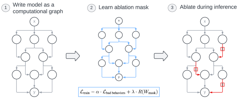
In this work, we propose a new method for removing undesirable behaviors: targeted edge ablation. In targeted edge ablation, we target a bad behavior by removing a small number of causal pathways through the model at inference time (Figure 1). Targeted edge ablation follows recent work in using causal mediation to discover computational circuits responsible for particular model behaviors (Wang et al., 2022; Goldowsky-Dill et al., 2023; Geiger et al., 2023a). Rather than discovering circuits, targeted edge ablation discovers causal cuts through circuits, disabling circuits responsible for bad behaviors.

Main Contributions.

We formulate the problem of behavior removal and propose targeted edge ablation as a possible solution (Section 3). We then present preliminary results in performing targeted edge ablation to harm performance in toxic language generation (Section 4).

2 Background

Circuit analysis.

We can write any model as a connected directed acyclic graph (DAG) with source nodes representing the model’s (typically vector-valued) input, sink nodes representing the model’s output, and intermediate nodes representing units of computation (e.g. Figure 1, left; see Appendix B). Circuit analysis attempts to mechanistically understand model computation by identifying a subgraph of this DAG that is responsible for a given behavior, and assigning semantic meaning to (groups of) nodes (Wang et al., 2022; Räukur et al., 2022; Chan et al., 2022). Circuits have also been discussed in the context of treating nodes as “features,” usually defined as directions in the latent space (Olah, 2022; Cammarata et al., 2020).

Ablating edges in a computational graph.

Since edges in the model’s computational graph represent dependencies between nodes, we can simulate what the model would have computed without a certain node-to-node dependency by performing ablation on an edge in the graph. While previous work has largely focused on ablation of nodes (Ghorbani & Zou, 2020), an advantage of our strategy of ablating edges rather than nodes is the mitigation of polysemantic behavior of model components (Olah et al., 2020), since we investigate the causal importance of each causal path into and out of the component. In our experiments, we use zero ablation, in which we compute the destination node as if the source node’s value were zero, and mean ablation (Wang et al., 2022), in which we compute the destination node as if the source node’s value were set to its mean value over the training set. See Appendix C for more.

3 Targeted Ablation for Behavior Removal

Let $\mathcal{L}(M,\mathcal{D})$ indicate the loss of model $M$ on a distribution $\mathcal{D}$ over input-label pairs. We specify a behavior as some distribution $\mathcal{D}$ on which the model achieves low loss $\mathcal{L}(M,\mathcal{D})<K$ for some appropriate hyperparameter $K$ . We can define the disjointness $\delta(\mathcal{D},\mathcal{D}^{\prime})$ for behaviors $\mathcal{D}$ and $\mathcal{D}^{\prime}$ to be the total variation distance between $\mathcal{D}$ and $\mathcal{D}^{\prime}$ . In particular, the total variation distance is 1 if $\mathcal{D}$ assigns probability 0 to all regions that $D^{\prime}$ assigns positive probability and vice versa.

Definition 3.1 (Behavior Removal).

Given a model $\mathcal{M}$ and unlimited access to training samples, produce a model $\mathcal{M}^{*}$ which achieves high loss $\mathcal{L}(\mathcal{M}^{*},\mathcal{D})>K$ , without harming distinct behaviors. In particular, for all behaviors $\mathcal{D}^{\prime}$ completely disjoint from $\mathcal{D}$ , i.e. $\delta(\mathcal{D},\mathcal{D}^{\prime})=1$ , we wish to preserve $\mathcal{L}(\mathcal{M}^{*},\mathcal{D}^{\prime})\leq\mathcal{L}(\mathcal{M},\mathcal{D}^{\prime})$ .

Thus, behavior removal has two goals: efficacy – the edited model should achieve high loss on $\mathcal{D}$ ; and specificity – the edited model should achieve low loss on all disjoint behaviors $\mathcal{D}^{\prime}$ for which the original model achieves low loss.

Let $D_{\text{train}}$ be our train set, and $D_{\text{behavior}}$ be samples from $\mathcal{D}$ . One reason the model might exhibit a behavior is if $\mathcal{D}$ overlaps with the training distribution, which would incentivize the model to produce low loss on $\mathcal{D}$ . Thus, it is reasonable to assume $D_{\text{train}}$ and $\mathcal{D}$ may not be completely disjoint.

3.1 Baseline: Finetuning

We form an approximate objective function by encouraging preserving performance on the training set, while increasing loss on the bad behavior set:

\mathcal{L}(\mathcal{M},D_{\text{train}})-\alpha\cdot\mathcal{L}(\mathcal{M},D_{\text{behavior}})

(1)

where $\alpha$ is a hyperparameter. We can now finetune using Equation 1. Since $D_{\text{behavior}}$ is often small, we use early stopping to avoid overfitting.

3.2 Baseline: Task Arithmetic

In task arithmetic (Ilharco et al., 2023), we finetune $\mathcal{M}$ on $\mathcal{L}(\mathcal{M},D_{\text{behavior}})$ towards the bad behaviors, and find the “task vector”, or difference in weights between the finetuned model and $\mathcal{M}$ . We then form $\mathcal{M}^{*}$ by adding the negated task vector to $\mathcal{M}$ .

3.3 Targeted Edge Ablation

Following Figure 1, we describe targeted edge ablation as three steps.

1. Rewrite the model. We first choose at what level of granularity to represent the model’s computation. Since we learn a mask over edges in the resulting graph, increasing the granularity results in a more expressive ablation process. We call the specified graph $G$ , and call its set of edges $E_{G}$ .

2. Learn an ablation mask. Let $G_{-E}$ be our graph $G$ with the edges in $E$ ablated. Then we wish to select $E\subset E_{G}$ that minimizes

\displaystyle\mathcal{L}(G_{-E},D_{\text{train}})-\alpha\cdot\mathcal{L}(G_{-E},D_{\text{behavior}})+\lambda\cdot R(E)

(2)

for hyperparameters $\alpha,\lambda$ and some regularization function $R$ .¹¹1The regularization term penalizes large sizes of $E$ to apply pressure to find a minimal subset of edges that disables the behavior. To compute an optimal edge subset $E$ , we optimize an edge mask $W_{\text{mask}}$ on a continuous relaxation of Equation 2. Every edge $e=(A,B)$ is given a learnable weight $w_{e}\in[0,1]$ , where $w_{e}=0$ corresponds to ablating $e$ , $w_{e}=1$ corresponds to preserving $e$ , and $0<w_{e}<1$ corresponds to node $B$ observing the following convex combination of the preserved value ( $v_{A}$ ) and the ablated value ( $\mu_{A}$ ) for node $A$ :

w_{e}\cdot v_{A}+(1-w_{e})\cdot\mu_{A}

(3)

When $w_{e}=0$ , node $B$ ’s observation of node $A$ is replaced by its ablated value, and when $w_{e}=1$ , node $B$ fully observes the value of node $A$ . We initialize the mask parameters $W_{\text{mask}}$ to a vector of 1s (indicating fully faithful model computation) and train $W_{\text{mask}}$ on the loss function

$\displaystyle\mathcal{L}(W_{\text{mask}};\alpha,\lambda,R)=\$	$\displaystyle\mathcal{L}(W_{\text{mask}},D_{\text{train}})$
	$\displaystyle-\alpha\cdot\mathcal{L}(W_{\text{mask}},D_{\text{bad behavior}})$
	$\displaystyle+\lambda(t)\cdot R(W_{\text{mask}})$	(4)

We train with a regularization weight $\lambda(t)$ that increases over time, since we find that this training dynamic encourages the edge mask to find a set of ablations that removes the bad behavior and then revise it to minimize the number of ablations. When training is finished, we then round all the mask weights to either 0 or 1 by selecting the set of ablated edges to be $\hat{E}^{*}=\{e\ |\ w_{e}\leq\tau\}$ for some threshold $\tau\in(0,1)$ .

3. Ablate during inference. We form $\mathcal{M}^{*}$ by ablating the edges learned in step (2) at inference time.

3.4 Conceptual Advantages over Fine-Tuning

Limited Expressivity.

LMs and other large models may have millions or billions of parameters and thus may be vastly overparameterized for the task of performing poorly on the bad-behavior examples, especially if generating bad-behavior examples is expensive and the set of examples is small.²²2For example, collecting jailbreaks to remove jailbreaking behavior is challenging and expensive.

A particular advantage of limiting the expressivity of our solution class is avoiding the negative effects of training on a mis-specified objective function like Equation 1, which encourages low loss on samples in $D_{\text{train}}$ which exhibit the behavior but are not included in $D_{\text{behavior}}$ . Allowing the model to overfit to this loss function may result in memorization of the points in $D_{\text{behavior}}$ to maintain low loss on all of $D_{\text{train}}$ , including those points which have high likelihood in $\mathcal{D}$ . On the other hand, edge ablation limits the expressivity of the solution space and relies on the model’s previously learned specialization of causal pathways.

Preserving Structure.

Since edge ablation edits the model at a high level, it preserves most of the model’s mechanistic calculus. Even subtle fine-tuning has the potential to entirely reorganize the model’s reasoning process, disrupting any mechanistic interpretability work that has already been performed. Targeted edge ablation is unlikely to induce the model to change its reasoning structure or increase its knowledge because it strictly decreases the amount of information available to the model’s computation.

4 Removing Toxicity in GPT-2

We apply our model editing methodology to preventing the generation of toxic (e.g. offensive, swear-filled) sequences in a pre-trained GPT-2 Small (Radford et al., 2019). Our goal is to edit GPT-2 so that it achieves high loss on toxic sequences, so our $\mathcal{D}$ is a distribution over toxic sequences for which the model achieves low loss.³³3All code is available at https://github.com/xanderdavies/circuit-breaking.

As an approximation of our train set $D_{\text{train}}$ , we use 10,000 samples from OpenWebText (OWT) (Gokaslan & Cohen, 2019). See Appendix E for results in removing a sub-class in an image classification model.

Constructing a bad behavior dataset.

We sample excerpts from highly toxic comments posted to the Politically Incorrect board of 4chan imageboard forum (Papasavva et al., 2020). We sample from posts assigned a toxicity score of greater than 0.9, as calculated by Google’s Perspective API Toxicity V6 (Google, 2023).

4.1 Learning Edge Mask Details

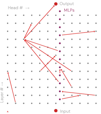
Similar to (Goldowsky-Dill et al., 2023; Wang et al., 2022), we write GPT-2 as a graph consisting of the input, the output, attention heads, and MLPs (158 nodes total) by considering a “residual rewrite” of the model’s computational structure. The canonical description of a transformer model expresses the attention head $A_{i,j}$ (the $j$ th attention head in layer $i$ ) as taking an argument $R_{i-1}$ , the residual from the previous layer. However, since $R_{0}=I$ (where $I$ represents the input embeddings) and $R_{i}=R_{i-1}+\sum_{j}A_{i,j}+M_{i}$ (where $M_{i}$ is the output of the MLP node in layer $i$ ), we can instead consider attention head $A_{i,j}$ as operating on the sum $S^{A}_{i}=I+\sum_{i^{\prime}<i}\left(M_{i^{\prime}}+\sum_{j^{\prime}}A_{i^{\prime},j^{\prime}}\right)$ , and taking all nodes in previous layers as separate input arguments. Similarly, we can consider MLP node $M_{i}$ as operating on the sum $S^{M}_{i}=I+\sum_{i^{\prime}<i}M_{i^{\prime}}+\sum_{i^{\prime}\leq i}\sum_{j^{\prime}}A_{i^{\prime},j^{\prime}}$ , and the output node as operating on the sum of the input embeddings and all attention head and MLP outputs. In total, this residual rewrite gives us a nearly-dense graph containing 11,611 edges: one between every pair of (attention head, MLP, input, and output) nodes, except for attention heads in the same layer, which do not communicate with each other. Concretely, ablating an edge from $A_{i^{\prime},j^{\prime}}$ to $A_{i,j}$ entails replacing the $A_{i^{\prime},j^{\prime}}$ term in $S^{A}_{i}$ for the input to attention head $A_{i,j}$ with zero (for zero ablation) or the mean value of head $A_{i^{\prime},j^{\prime}}$ (for mean ablation).

We train two ablated models using a continuous edge mask. First, we train a zero-ablation mask against $\mathcal{L}(W_{\text{mask}};\alpha,\lambda,R)$ described in equation 4, with $\alpha=0.2$ , $\lambda(t)=(t-20)/10000$ , and $R(W_{\text{mask}})=\sum_{e\in E_{G}}w_{e}$ . This search process finds a mask that ablates 12 edges (Figure 2) and mitigates toxicity while preserving coherence. Second, we train a mean-ablation mask with $\alpha=0.15$ and using the same hyperparameters otherwise, which finds a mask that ablates 84 edges and produces a similar effect.

As a baseline, we fine-tune on the loss given by Equation 1 directly, with $\alpha=0.2$ . We use early stopping with a validation set to prevent overfitting.⁴⁴4We note this is a stronger baseline than naively training for high loss on our bad behavior set as done in (Ilharco et al., 2023), which we call “gradient ascent” in Table 1. We also compare to task arithmetic (Ilharco et al., 2023) (Section 3.2).

	Toxic-loss	Toxic-loss (filtered)	Toxic generation	Toxic generation (filtered)	Incoherence	TPP Incoherence
Original	4.954	4.435	0.453	0.944	4.264	4.617
Gradient Ascent	21.339	20.980	0.015	0.013	15.287	18.415
Task Arithmetic	5.357	4.827	0.351	0.631	4.427	4.731
Joint Fine-Tuned	11.817	13.020	0.009	0.008	4.240	7.402
Ablated (12 edges)	5.027	4.486	0.328	0.567	4.280	4.623
Ablated (84 edges)	4.895	4.470	0.280	0.441	4.180	4.515

Table 1: Toxic-loss measures the model’s loss on toxic prompts. Toxic generation measures the average toxicity score of model generations on toxic prompts, according to the Detoxify classifier. The filtered columns denote the loss or generation toxicity on test samples filtered by the original model achieving low loss (

<5

) or highly toxic generation (

>.9

). Incoherence measures the model’s loss on OWT. Toxic Pre-Pended (TPP) incoherence measures the model’s loss after on OWT sequences that have been preceded by toxic text.

4.2 Evaluation Metrics

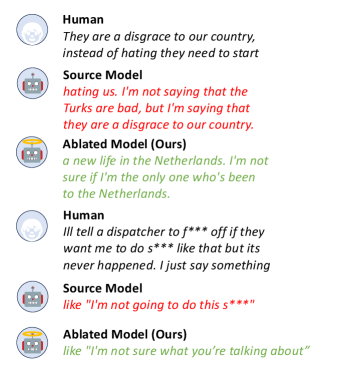
Following Definition 3.1, we evaluate both the model’s avoidance of toxic generation (efficacy) and the detriment to other behaviors (specificity). Since our goal is for the ablated model to achieve high loss on all toxic sequences (i.e. minimizing its probability of predicting subsequent tokens that would cause the sequence to be toxic), we evaluate efficacy in a few ways. First, we consider the ablated model’s loss on with-held toxic text and in particular its loss on sequences for which the original model achieves low ( $<5$ ) loss. Second, we consider the toxicity of the model’s completions when prompted with toxic text, as measured by the score in $[0,1]$ , 0 being the least toxic, given by the toxic-comment classifier Detoxify. We emphasize the toxicity of model completions on the specific prompts for which the original model produces highly toxic ( $>0.9$ ) output.

We evaluate specificity by using the perplexity on withheld sequences from OWT, along with the perplexity on withheld OWT sequences prepended with toxic content. The original model produces low loss (4.617) on these sequences, and we choose to highlight the behavior of retaining coherence when prompted with toxic text as one that is particularly likely to be inadvertently removed when editing the model to produce high loss on toxic text.

4.3 Results

Results are shown in Table 1. We train a model with 12 edges zero-ablated that substantially mitigates toxic generation, decreasing the average toxicity score on model generations for toxic prompts from 0.458 to 0.328 and in particular for the most toxic-inducing prompts from 0.944 to 0.567. This minimal edge ablation outperforms task arithmetic on every efficacy and specificity metric, and causes a lower increase in incoherence following toxic prompts than joint fine-tuning, though it does not eradicate the model’s toxicity. Our mean-ablation mask with 84 edges achieves a similar result, greatly mitigating toxic generations without detracting from the model’s other behaviors.

5 Related Work

Causal mediation for circuit analysis.

Causal mediation (Pearl, 2009; Iwasaki & Simon, 1994) has been proposed as a framework for evaluating mechanistic causal explanations for model outputs (Goldowsky-Dill et al., 2023; Geiger et al., 2023a; Vig et al., 2020). Experimental evaluation for causal explanations involves performing a set of ablation experiments to check whether they match hypothesized effects. For example, ablating allegedly unimportant paths should have little impact on the target behavior. Previous work has used the causal mediation framework to discover circuits, including in transformers (Chan et al., 2022; Wang et al., 2022; Nanda et al., 2023).

Existing causal mediation tests and circuit discovery methods built upon these tests evaluate whether a given set of edges are sufficient for a given model behavior (i.e. if they contain a vertical path along the circuit), while our circuit breaking technique finds a set of edges that are necessary for the behavior (i.e. a horizontal “cut” through the circuit).

Automated circuit discovery.

Recent work has explored automated approaches to discovering circuits, including greedy algorithms which crawl the computational graph and remove edges which preserve behavior above a fixed threshold (Conmy et al., 2023), and gradient descent-based methods which use interchange intervention training (Geiger et al., 2022) to learn alignments between a source model and a proposed high-level causal model (Geiger et al., 2023b). Our work differs in attempting to find neither single features (Vig et al., 2020; Gurnee et al., 2023) nor full computational circuits (Geiger et al., 2023b; Goldowsky-Dill et al., 2023; Wang et al., 2022); instead we discover edges where removing their causal effect breaks a given behavior.

Weight-masking and model pruning.

Much prior work has sought to compress models by masking parameters (LeCun et al., 1989; Hassibi & Stork, 1992). Most relevant to our work are approaches which learn masks from data by encouraging sparsity and preserving performance (Louizos et al., 2017; Wang et al., 2019; Cao et al., 2021). In our work, we disincentivize sparsity (since we want fewer ablations), and use an objective function tailored to removing a specific behavior instead of preserving general performance. Additionally, our edge-masking technique is more general than weight-masking, since we can ablate internal connections between high-level model components that do not correspond directly to particular weights, such as communication channels between pairs of attention heads. Finally, we prune using mean ablation instead of zero ablation.

Model editing to change or remove behaviors.

Recent work has made changes to model behavior by making targeted edits to model weights (Meng et al., 2022) or activations (Hernandez et al., 2023), which differ from our goal of removing behaviors. (Gandikota et al., 2023) propose a fine-tuning approach to erasing concepts from diffusion models. (Elazar et al., 2021) remove information from a language model’s representation by iteratively learning linear probes to extract the information and projecting onto the null space. Compared to such work, we consider coarser ablations, allow editing around multiple components, and seek to break behaviors as opposed to erasing information. Like us, (Ilharco et al., 2023) attempt to remove the toxic generation behavior in GPT-2, but do so by fine-tuning on bad behavior and subtracting the weight-difference from the original model.

6 Conclusion

Using a small dataset of examples of inputs on which a neural network exhibits a “bad behavior,” we find that our method can make high-level modifications to the network that mitigate the bad behavior on the provided examples, generalize to removing the bad behavior across other inputs that trigger it, and cause only small amounts of damage to the model’s performance on all other inputs (see D for limitations). We conjecture that model editing may be an alternate tool for targeted behavioral modification to fine-tuning, and encourage future work further investigating our approach.

References

Bourtoule et al. (2021) Bourtoule, L., Chandrasekaran, V., Choquette-Choo, C. A., Jia, H., Travers, A., Zhang, B., Lie, D., and Papernot, N. Machine unlearning. In 2021 IEEE Symposium on Security and Privacy (SP), pp. 141–159. IEEE, 2021.
Brown et al. (2020) Brown, T. B., Mann, B., Ryder, N., Subbiah, M., Kaplan, J., Dhariwal, P., Neelakantan, A., Shyam, P., Sastry, G., Askell, A., Agarwal, S., Herbert-Voss, A., Krueger, G., Henighan, T., Child, R., Ramesh, A., Ziegler, D. M., Wu, J., Winter, C., Hesse, C., Chen, M., Sigler, E., Litwin, M., Gray, S., Chess, B., Clark, J., Berner, C., McCandlish, S., Radford, A., Sutskever, I., and Amodei, D. Language models are few-shot learners, 2020.
Cammarata et al. (2020) Cammarata, N., Carter, S., Goh, G., Olah, C., Petrov, M., Schubert, L., Voss, C., Egan, B., and Lim, S. K. Thread: circuits. Distill, 5(3):e24, 2020.
Cao et al. (2021) Cao, S., Sanh, V., and Rush, A. M. Low-complexity probing via finding subnetworks. arXiv preprint arXiv:2104.03514, 2021.
Chan et al. (2022) Chan, L., Garriga-Alonso, A., Goldowsky-Dill, N., Greenblatt, R., Nitishinskaya, J., Radhakrishnan, A., Shlegeris, B., and Thomas, N. Causal Scrubbing: a method for rigorously testing interpretability hypotheses [Redwood Research], December 2022. URL https://www.alignmentforum.org/posts/JvZhhzycHu2Yd57RN/causal-scrubbing-a-method-for-rigorously-testing.
Chen et al. (2018) Chen, J., Song, L., Wainwright, M. J., and Jordan, M. I. Learning to explain: An information-theoretic perspective on model interpretation, 2018.
Conmy et al. (2023) Conmy, A., Mavor-Parker, A. N., Lynch, A., Heimersheim, S., and Garriga-Alonso, A. Towards automated circuit discovery for mechanistic interpretability. arXiv preprint arXiv:2304.14997, 2023.
Covert et al. (2020) Covert, I., Lundberg, S., and Lee, S.-I. Understanding global feature contributions with additive importance measures, 2020.
Covert et al. (2022) Covert, I., Lundberg, S., and Lee, S.-I. Explaining by removing: A unified framework for model explanation, 2022.
Dabkowski & Gal (2017) Dabkowski, P. and Gal, Y. Real time image saliency for black box classifiers. In Guyon, I., Luxburg, U. V., Bengio, S., Wallach, H., Fergus, R., Vishwanathan, S., and Garnett, R. (eds.), Advances in Neural Information Processing Systems, volume 30. Curran Associates, Inc., 2017. URL https://proceedings.neurips.cc/paper_files/paper/2017/file/0060ef47b12160b9198302ebdb144dcf-Paper.pdf.
Deng (2012) Deng, L. The mnist database of handwritten digit images for machine learning research. IEEE Signal Processing Magazine, 29(6):141–142, 2012.
Devlin et al. (2019) Devlin, J., Chang, M.-W., Lee, K., and Toutanova, K. Bert: Pre-training of deep bidirectional transformers for language understanding, 2019.
Elazar et al. (2021) Elazar, Y., Ravfogel, S., Jacovi, A., and Goldberg, Y. Amnesic probing: Behavioral explanation with amnesic counterfactuals. Transactions of the Association for Computational Linguistics, 9:160–175, 2021.
Fong & Vedaldi (2017) Fong, R. C. and Vedaldi, A. Interpretable explanations of black boxes by meaningful perturbation. In 2017 IEEE International Conference on Computer Vision (ICCV). IEEE, oct 2017. doi: 10.1109/iccv.2017.371. URL https://doi.org/10.1109%2Ficcv.2017.371.
Gandikota et al. (2023) Gandikota, R., Materzynska, J., Fiotto-Kaufman, J., and Bau, D. Erasing concepts from diffusion models. arXiv preprint arXiv:2303.07345, 2023.
Geiger et al. (2022) Geiger, A., Wu, Z., Lu, H., Rozner, J., Kreiss, E., Icard, T., Goodman, N., and Potts, C. Inducing causal structure for interpretable neural networks. In International Conference on Machine Learning, pp. 7324–7338. PMLR, 2022.
Geiger et al. (2023a) Geiger, A., Potts, C., and Icard, T. Causal abstraction for faithful model interpretation, 2023a.
Geiger et al. (2023b) Geiger, A., Wu, Z., Potts, C., Icard, T., and Goodman, N. D. Finding alignments between interpretable causal variables and distributed neural representations. arXiv preprint arXiv:2303.02536, 2023b.
Ghorbani & Zou (2020) Ghorbani, A. and Zou, J. Neuron shapley: Discovering the responsible neurons, 2020.
Gokaslan & Cohen (2019) Gokaslan, A. and Cohen, V. Openwebtext corpus. http://Skylion007.github.io/OpenWebTextCorpus, 2019.
Golatkar et al. (2020) Golatkar, A., Achille, A., and Soatto, S. Eternal sunshine of the spotless net: Selective forgetting in deep networks. In Proceedings of the IEEE/CVF Conference on Computer Vision and Pattern Recognition, pp. 9304–9312, 2020.
Goldowsky-Dill et al. (2023) Goldowsky-Dill, N., MacLeod, C., Sato, L., and Arora, A. Localizing model behavior with path patching. arXiv preprint arXiv:2304.05969, 2023.
Google (2023) Google. Perspective API, 2023. URL https://perspectiveapi.com/.
Guan et al. (2022) Guan, J., Tu, Z., He, R., and Tao, D. Few-shot backdoor defense using shapley estimation. In Proceedings of the IEEE/CVF Conference on Computer Vision and Pattern Recognition, pp. 13358–13367, 2022.
Gurnee et al. (2023) Gurnee, W., Nanda, N., Pauly, M., Harvey, K., Troitskii, D., and Bertsimas, D. Finding neurons in a haystack: Case studies with sparse probing. arXiv preprint arXiv:2305.01610, 2023.
Hanu & Unitary team (2020) Hanu, L. and Unitary team. Detoxify. Github. https://github.com/unitaryai/detoxify, 2020.
Hassibi & Stork (1992) Hassibi, B. and Stork, D. Second order derivatives for network pruning: Optimal brain surgeon. Advances in neural information processing systems, 5, 1992.
Hernandez et al. (2023) Hernandez, E., Li, B. Z., and Andreas, J. Measuring and manipulating knowledge representations in language models. arXiv preprint arXiv:2304.00740, 2023.
Ilharco et al. (2023) Ilharco, G., Ribeiro, M. T., Wortsman, M., Gururangan, S., Schmidt, L., Hajishirzi, H., and Farhadi, A. Editing Models with Task Arithmetic, March 2023. URL http://arxiv.org/abs/2212.04089. arXiv:2212.04089 [cs].
Iwasaki & Simon (1994) Iwasaki, Y. and Simon, H. A. Causality and model abstraction. Artificial intelligence, 67(1):143–194, 1994.
Lakkaraju et al. (2016) Lakkaraju, H., Bach, S. H., and Leskovec, J. Interpretable decision sets: A joint framework for description and prediction. In Proceedings of the 22Nd ACM SIGKDD International Conference on Knowledge Discovery and Data Mining, KDD ’16, pp. 1675–1684, New York, NY, USA, 2016. ACM. ISBN 978-1-4503-4232-2. doi: 10.1145/2939672.2939874. URL http://doi.acm.org/10.1145/2939672.2939874.
LeCun & Cortes (2010) LeCun, Y. and Cortes, C. MNIST handwritten digit database. http://yann.lecun.com/exdb/mnist/, 2010. URL http://yann.lecun.com/exdb/mnist/.
LeCun et al. (1989) LeCun, Y., Denker, J., and Solla, S. Optimal brain damage. Advances in neural information processing systems, 2, 1989.
Louizos et al. (2017) Louizos, C., Welling, M., and Kingma, D. P. Learning sparse neural networks through $l\_0$ regularization. arXiv preprint arXiv:1712.01312, 2017.
Lundberg & Lee (2017) Lundberg, S. M. and Lee, S.-I. A unified approach to interpreting model predictions. In Guyon, I., Luxburg, U. V., Bengio, S., Wallach, H., Fergus, R., Vishwanathan, S., and Garnett, R. (eds.), Advances in Neural Information Processing Systems, volume 30. Curran Associates, Inc., 2017. URL https://proceedings.neurips.cc/paper/2017/file/8a20a8621978632d76c43dfd28b67767-Paper.pdf.
Meng et al. (2022) Meng, K., Bau, D., Andonian, A., and Belinkov, Y. Locating and editing factual associations in gpt. Advances in Neural Information Processing Systems, 35:17359–17372, 2022.
Nanda (2023) Nanda, N. Attribution patching: Activation patching at industrial scale, 2023. URL https://www.neelnanda.io/mechanistic-interpretability/attribution-patching.
Nanda et al. (2023) Nanda, N., Chan, L., Liberum, T., Smith, J., and Steinhardt, J. Progress measures for grokking via mechanistic interpretability. arXiv preprint arXiv:2301.05217, 2023.
Olah (2022) Olah, C. Mechanistic interpretability, variables, and the importance of interpretable bases. Transformer Circuits Thread(June 27). http://www. transformer-circuits. pub/2022/mech-interp-essay/index. html, 2022.
Olah et al. (2020) Olah, C., Cammarata, N., Schubert, L., Goh, G., Petrov, M., and Carter, S. Zoom in: An introduction to circuits. Distill, 2020. doi: 10.23915/distill.00024.001. https://distill.pub/2020/circuits/zoom-in.
OpenAI (2023) OpenAI. Gpt-4 technical report, 2023. URL https://arxiv.org/abs/2303.08774.
Ouyang et al. (2022) Ouyang, L., Wu, J., Jiang, X., Almeida, D., Wainwright, C., Mishkin, P., Zhang, C., Agarwal, S., Slama, K., Ray, A., et al. Training language models to follow instructions with human feedback. Advances in Neural Information Processing Systems, 35:27730–27744, 2022.
Papasavva et al. (2020) Papasavva, A., Zannettou, S., Cristofaro, E. D., Stringhini, G., and Blackburn, J. Raiders of the lost kek: 3.5 years of augmented 4chan posts from the politically incorrect board, 2020.
Pearl (2009) Pearl, J. Causality. Cambridge university press, 2009.
Poursabzi-Sangdeh et al. (2018) Poursabzi-Sangdeh, F., Goldstein, D. G., Hofman, J. M., Vaughan, J. W., and Wallach, H. M. Manipulating and measuring model interpretability. arXiv, abs/1802.07810, 2018. URL http://arxiv.org/abs/1802.07810.
Radford et al. (2019) Radford, A., Wu, J., Child, R., Luan, D., Amodei, D., Sutskever, I., et al. Language models are unsupervised multitask learners. OpenAI blog, 1(8):9, 2019.
Räukur et al. (2022) Räukur, T., Ho, A., Casper, S., and Hadfield-Menell, D. Toward transparent ai: A survey on interpreting the inner structures of deep neural networks. arXiv preprint arXiv:2207.13243, 2022.
Sekhari et al. (2021) Sekhari, A., Acharya, J., Kamath, G., and Suresh, A. T. Remember what you want to forget: Algorithms for machine unlearning. Advances in Neural Information Processing Systems, 34:18075–18086, 2021.
Shapley (1997) Shapley, L. S. A value for n-person games. Classics in game theory, 69, 1997.
Stiennon et al. (2022) Stiennon, N., Ouyang, L., Wu, J., Ziegler, D. M., Lowe, R., Voss, C., Radford, A., Amodei, D., and Christiano, P. Learning to summarize from human feedback, 2022.
Touvron et al. (2023) Touvron, H., Lavril, T., Izacard, G., Martinet, X., Lachaux, M.-A., Lacroix, T., Rozière, B., Goyal, N., Hambro, E., Azhar, F., Rodriguez, A., Joulin, A., Grave, E., and Lample, G. Llama: Open and efficient foundation language models, 2023.
Vig et al. (2020) Vig, J., Gehrmann, S., Belinkov, Y., Qian, S., Nevo, D., Singer, Y., and Shieber, S. Investigating gender bias in language models using causal mediation analysis. Advances in neural information processing systems, 33:12388–12401, 2020.
Wang et al. (2022) Wang, K., Variengien, A., Conmy, A., Shlegeris, B., and Steinhardt, J. Interpretability in the wild: a circuit for indirect object identification in gpt-2 small, 2022.
Wang et al. (2019) Wang, Z., Wohlwend, J., and Lei, T. Structured pruning of large language models. arXiv preprint arXiv:1910.04732, 2019.
Wu & Wang (2021) Wu, D. and Wang, Y. Adversarial neuron pruning purifies backdoored deep models. Advances in Neural Information Processing Systems, 34:16913–16925, 2021.
Yoon et al. (2019) Yoon, J., Jordon, J., and van der Schaar, M. INVASE: Instance-wise variable selection using neural networks. In International Conference on Learning Representations, 2019. URL https://openreview.net/forum?id=BJg_roAcK7.
Zhou et al. (2015) Zhou, B., Khosla, A., Lapedriza, A., Oliva, A., and Torralba, A. Object detectors emerge in deep scene cnns, 2015.
Ziegler et al. (2022) Ziegler, D. M., Nix, S., Chan, L., Bauman, T., Schmidt-Nielsen, P., Lin, T., Scherlis, A., Nabeshima, N., Weinstein-Raun, B., de Haas, D., Shlegeris, B., and Thomas, N. Adversarial training for high-stakes reliability, 2022.

Appendix A Additional Related Work

Unlearning.

Machine unlearning aims to modify a model to match the behavior of a model which had not seen certain data points (Sekhari et al., 2021; Bourtoule et al., 2021; Golatkar et al., 2020). However, a key difference in our setting is that we are not able to enumerate the full set of undesirable data points in our training set.

Backdoor removal.

(Wu & Wang, 2021) learn a binary mask to zero ablate neurons sensitive to adversarial perturbations, and finds that doing so removes injected backdoors. (Guan et al., 2022) target backdoors by estimating Shapley importance values (Shapley, 1997) for every edge and then zero ablating neurons which have a high attack success rate attribution score, finding they are able to remove backdoors with very limited (and sometimes no) data. We believe our technique could be effective for disabling the activation of backdoor mechanisms and find this application a promising direction for future work.

Appendix B Writing models as computational graphs.

We can write any model as a connected directed acyclic graph (DAG) with source nodes representing the model’s (typically vector-valued) input, sink nodes representing the model’s output, and intermediate nodes representing units of computation. Each intermediate node represents a function of the values of its parent nodes. On a forward pass, given values for its input nodes, the model computes the value of each node in any topologically sorted order until it has computed the value of the output nodes.

For any model, there are many equivalent graphs that faithfully represent its computation. In particular, a computational graph can represent a model at varying levels of detail. At one extreme, intermediate nodes can designate individual additions, multiplications, and nonlinearities – such a graph would have at least as many nodes as model parameters. On the other hand, many model architectures have self-contained computational modules, which allows them to be represented by graphs that convey a high level of abstraction. For example, in convolutional networks, intermediate nodes can represent convolutional filters and pooling layers, while in transformer models (Devlin et al., 2019), the natural high-level computational units are attention heads and multi-layer perceptron (MLP) modules. To be more granular, we can subdivide each attention head node into nodes that compute queries, keys, and values and combine them into attention patterns (Figure 3).

Appendix C Ablation Types

One mode of ablating an edge is zero ablation, in which we compute the value of its destination node as if the value of its source node were zero. However, a value of zero on an intermediate node can sometimes be highly unusual, and can thus in some cases convey a strong idiosyncratic signal to the destination node.

One other technique is mean ablation, in which we compute the destination node as if the source node’s value were set to its mean value over the training set. Mean ablation arguably better captures a lack of information flow: if the specific value of the source node were withheld from the destination node, the source node’s mean value would be the most general estimate of its true value.

Appendix D Limitations

We ablate edges by setting their input values to zero and the train-set mean. However, recent work has argued that ablating model components with random samples from their marginal distributions may be preferable and that mean ablation may lead to out of distribution resampling (Goldowsky-Dill et al., 2023). Additionally, circuit-breaking interventions on the model could be made even more surgical by using more granular model nodes and edges (for example, splitting attention heads into query, key, and value nodes). Finally, our results could be strengthened by considering stronger baselines and additional approaches to learning binary masks.

Appendix E Additional Experiments: Breaking Digit Classification in an MLP

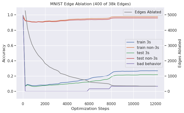
We train a one-hidden-layer MLP with a 50 hidden neurons to classify the handwritten digits of MNIST, then use a small (30 example) dataset of a particular digit (say, 3) to remove the model’s ability to correctly classify that digit. We consider the most granular computational graph for the MLP with one node for each pixel of the input, one for each hidden neuron, and one for each output neuron. The graph contains an edge corresponding to each weight in the network. To prevent our learned mask from simply ablating the edges feeding into the output neuron corresponding to 3, we arbitrarily pair digits and merge their labels so that the MLP has only 5 output neurons rather than 10. This pairing forces the network to retain edges to the output neuron that aid in correctly classifying the digit that is paired with 3, while not using the neuron for the 3 inputs.

We search for a binary mask over edges by training a continuous edge mask against $\mathcal{L}(W_{\text{mask}};\alpha,\lambda,R)$ described in Equation 4. Specifically, we use $\alpha=0.3$ , $\lambda(t)=t$ , and $R(W_{\text{mask}})=\sum_{e\in E_{G}}\sqrt{1-w_{e}}$ . The sublinear cost imposed by $R$ incentivizes masks that are binary and ablate few edges; conceptually, if the mask were half-ablating two edges, it would receive a lower penalty for instead ablating one edge completely. We set the rounding threshold $\tau=0.5$ .

Using this technique, we find a binary mask that ablates 400 of the model’s 38K edges, bringing its accuracy on held-out “3”s from near-perfect to 21% (20% is random classification on this task), while accuracy on other (held-out) inputs stays high (dropping from 99% to 97%). We consider this a modest success for both the efficacy of the edit (i.e. its ability to transfer to other inputs on which the model exhibits the bad-behavior of classifying a “3” correctly) and also its specificity (i.e. the model’s continued ability to classify non-“3”s correctly) – see Figure 4.