Circular strings in Kerr- $AdS_{5}$ black holes

O. V. Geytota The Bogoliubov Laboratory of Theoretical Physics, JINR,
141980 Dubna, Moscow region, Russia Dubna State University
Universitetskaya str.,141980 Dubna, Moscow region, Russia A. A. Golubtsova The Bogoliubov Laboratory of Theoretical Physics, JINR,
141980 Dubna, Moscow region, Russia Steklov Mathematical Institute, Russian Academy of Sciences
Gubkina str. 8, 119991 Moscow, Russia H. Dimov The Bogoliubov Laboratory of Theoretical Physics, JINR,
141980 Dubna, Moscow region, Russia Department of Physics, Sofia University,
5 J. Bourchier Blvd., 1164 Sofia, Bulgaria Vu H. Nguyen The Bogoliubov Laboratory of Theoretical Physics, JINR,
141980 Dubna, Moscow region, Russia Institute of Physics, VAST, 10000 Hanoi, Vietnam R. C. Rashkov ¹¹1Emails: golubtsova, dimov @theor.jinr.ru and h_dimov,rash@phys.uni-sofia.bg Department of Physics, Sofia University,
5 J. Bourchier Blvd., 1164 Sofia, Bulgaria Institute for Theoretical Physics, Vienna University of Technology,
Wiedner Hauptstr. 8–10, 1040 Vienna, Austria

Abstract

The quest for extension of holographic correspondence to the case of finite temperature naturally includes Kerr-AdS black holes and their field theory duals. We probe the five-dimensional Kerr-AdS space time by pulsating strings. First we find particular pulsating string solutions and then semi-classically quantize the theory. For the string with large values of energy, we use the Bohr-Sommerfeld analysis to find the energy of the string as a function of a large quantum number. We obtain the wave function of the problem and thoroughly study the corrections to the energy, which according to the holographic dictionary are related to anomalous dimensions of certain operators in the dual gauge theory. The interpretation of results from holographic point of view is not straightforward since the dual theory is at finite temperature. Nevertheless, near or at conformal point the expressions can be thought of as the dispersion relations of stationary states.

1 Introduction

The intensive development of the gauge/gravity correspondence has yielded useful toolkits for exploring non-perturbative regime of quantum field theories. The gauge/gravity duality states that all the physics in a d-dimensional conformal gauge theory at strong coupling can be described in terms of a gravitational theory in a $(d+1)$ -dimensional spacetime with certain asymptotics. In particular, the dynamics of the 4d $\mathcal{N}=4$ $SU(N)$ SYM in the strong coupling regime is equivalent to the dynamics of the classical IIB superstring theory on $AdS_{5}\times S^{5}$ in the weakly coupled regime. This provides a dictionary between observables of the dual theories, which gives an opportunity to probe non-perturbative dynamics of gauge theories. An important class of observables includes various closed string configurations which energy spectrum can be related to anomalous dimensions of single-trace local operators in SYM. Despite that computing the string spectrum even in asymptotically AdS backgrounds is an intricate problem, the integrability methods used within the holographic duality allowed to find and analyze many string configurations.

Addressing the important issues as strong coupling phenomena, it became of great interest to extend the holographic duality to the case of finite temperature, which generically has less symmetries and phenomenologically more appropriate. Thermal observables contain a lot of information on dynamics of the system, however, they seems to be difficult to compute. The AdS/CFT correspondence allows to relate characteristics of black black holes in asymptotically AdS spacetimes to observables of strongly coupled quantum systems. The solutions are assumed to describe thermal states of the dual CFT with certain Hawking temperature. The use of the AdS/CFT correspondence appears to be a powerful method to investigate the thermal states of CFT. Indeed, the horizon is playing the role of a thermal background. This approach allows to include more dimensionless parameters in the theory making it very useful not only to collect important information for a higher dimensional theory but also to study its holographic dual. Particularly, the AdS black holes with spherical horizon are dual to the thermal ensemble of $\mathcal{N}=4$ SYM on $\mathbb{S}^{1}\times\mathbb{S}^{3}$ , while a planar AdS black brane is dual to finite-temperature $\mathcal{N}=4$ SYM on $\mathbb{S}^{1}\times\mathbb{R}^{3}$ [1, 2]. An intriguing suggestion has been made in [3], namely to consider a 5d Kerr-AdS black hole with a non-zero angular momentum as a gravity dual to "a rotating Einstein universe" on $\mathbb{R}\times\mathbb{S}^{3}$ . As a higher dimensional black hole the Kerr- $AdS_{5}$ black hole solution is characterized by two rotational parameters, related to the two parts of the angular momenta independently preserving. These parameters can be associated to the rotation in different planes. Note, that Kerr-AdS black holes share with non-rotating AdS black holes a number of common interesting features including the Hawking-Page phase transition, scaling of the free energy [4] and found its application in a holographic description of a rotating quark-gluon plasma [5]-[10]. At high temperatures the conformal symmetry is restored, so this description seems to be viable.

Certain thermal holographic observables can be found considering string dynamics in the black hole backgrounds. Circular closed strings in AdS black holes have been discussed in [11, 12]. Instead of rotating strings in the pure AdS case, the strings in the black holes are orbiting in these backgrounds. In particular, orbiting strings outside the 5d AdS-Schwarzschild black holes were interpreted as states of large spins in the dual thermal ensemble of $\mathcal{N}=4$ SYM theory on $\mathbb{S}^{1}\times\mathbb{S}^{3}$ . For the case of rotating AdS black holes the thermodynamical stability of closed string in the 5d Kerr-AdS black holes was studied with respect to angular momentum leakage to the black hole. A generalization of a pulsating string [19, 20, 21, 22] to the 5d AdS-Schwarzschild background was suggested in [12]. Following the Bohr-Sommerfeld quantization the energy of the string was computed, this energy can be associated with dispersion relations of the states in the $\mathcal{N}=4$ SYM theory at finite temperature.

In this paper we study pulsating string configurations in the 5d Kerr-AdS black hole with equal rotational parameters. We construct a pulsating string solution in the black hole background. We also compute the string energy reducing the string Nambu-Goto action to the mechanical Lagrangian and applying the Bohr-Sommerfeld analysis. The potential wells are related to the position of the outer black hole horizon and the boundary of the black hole spacetime. We derive the relation for the energy for the case of a small value of the rotational parameters. In the case of vanishing rotation this relation for the energy comes to that one obtained earlier in the work [12]. Note, that for the pure AdS case the energy of the string can be related to the anomalous dimensions of single trace operators in $\mathcal{N}=4$ SYM theory. In the black hole case we cannot establish this connection, since the notion of the anonymous dimension is defined in the conformal point. However, we can think on its relevance to the dispersion relations of the states in the thermal ensemble of $\mathcal{N}=4$ SYM theory on $\mathbb{S}^{1}\times\mathbb{S}^{3}$ . We also perform a WKB approximation and obtain the Schrödinger equation on the reduced subspace $y=const$ .

The paper is organized as follows. In Section 2 we give a review of the Kerr- $AdS_{5}$ black hole with equal rotational parameters. Section 3 is devoted to a pulsating string solutions, we present solutions for a pulsating string in the Kerr- $AdS_{5}$ . In Section 4 we consider the Bohr-Sommerfeld analysis and the WKB approximation. Finally, in Section 5 we conclude. In appendices we collect a number of useful relations for our computations.

2 5d Kerr-AdS black hole geometry

The 5d Kerr-AdS black hole solution was constructed in [3] and describes a rotating black hole with an AdS asymptotic. The metric of the 5d Kerr-AdS black holes is characterized by two rotational parameters $a$ , $b$ , related to the Casimirs of $SU(2)\times SU(2)\simeq SO(4)$ . In present paper we focus on the case of equal rotational parameters $a=b$ . The metric in the so-called AdS coordinates (static-at-infinity frame) can be represented as follows

	$\displaystyle ds^{2}$	$\displaystyle=$	$\displaystyle-(1+y^{2}\ell^{2})dT^{2}+y^{2}(d\Theta^{2}+\sin^{2}\Theta d\Phi^{2}+\cos^{2}\Theta d\Psi^{2})$
		$\displaystyle+$	$\displaystyle\frac{2M}{y^{2}\Xi^{3}}(dT-a\sin^{2}\Theta d\Phi-a\cos^{2}\Theta d\Psi)^{2}+\frac{y^{4}dy^{2}}{y^{4}(1+y^{2}\ell^{2})-\frac{2M}{\Xi^{2}}y^{2}+\frac{2Ma^{2}}{\Xi^{3}}},$

where

\Xi=1-a^{2}\ell^{2},

(2.2)

$M$ is the mass of the black hole, $a$ is a rotational parameter and we use the Hopf coordinates to parametrize the metric on the sphere with $0\leq\Theta\leq\frac{\pi}{2}$ , $0\leq\Phi,\Psi\leq 2\pi$ . Like ordinary Kerr solutions Kerr-AdS black holes have inner and outer horizons. We consider, that the holographic radial coordinate $y$ with values on the region $(y_{+},+\infty)$ , where $y_{+}$ is an outer horizon of the black hole and we reach an AdS-asymptotics as $y$ goes to $+\infty$ .

The position of the outer horizon in these coordinates is defined by a largest root of the equation ²²2We present the solutions to this equation in Appendix B.

1+y^{2}\ell^{2}-\frac{2M}{\Xi^{2}y^{2}}+\frac{2Ma^{2}}{\Xi^{3}y^{4}}=0.

(2.3)

Particularly, for the extremal 5d Kerr-AdS black hole the horizon is given by

y^{2}_{\rm+,ext}=\frac{1}{4\Xi}\left[4a^{2}\ell^{2}-1+\sqrt{1+8a^{2}\ell^{2}}\right].

(2.4)

From (2) it is easy to see that with $y\to\infty$ the 4d boundary of 5d Kerr-AdS black hole is 4d $R\times S^{3}$ [4, 15]

ds^{2}=-dT^{2}+d\Theta^{2}+\sin^{2}\Theta d\Phi^{2}+\cos^{2}\Theta d\Psi^{2}.

(2.5)

The Hawking temperature of the Kerr-AdS black hole is given by

T_{H}=\frac{1}{2\pi}\left(\frac{2y_{+}(1+y^{2}_{+}\ell^{2})}{(y^{2}_{+}+a^{2})}-\frac{1}{y_{+}}\right).

(2.6)

The angular momentum and the angular velocity are given by

J=\frac{\pi Ma}{\Xi^{3}},\quad\Omega=\frac{a(1+y^{2}_{+}\ell^{2})}{y^{2}_{+}+a^{2}},

(2.7)

correspondingly. Note, that there is a Hawking-Page phase transition in the Kerr-AdS black hole, and the rotation has an influence on it [9].

Taking $M=0$ in the 5d Kerr-AdS solution (2) we get

ds^{2}=-(1+y^{2}\ell^{2})dT^{2}+y^{2}(d\Theta^{2}+\sin^{2}\Theta d\Phi^{2}+\cos^{2}\Theta d\Psi^{2})^{2}+\frac{dy^{2}}{(1+y^{2}\ell^{2})},

(2.8)

that is merely the global representation of the AdS metric.

The 5d Kerr-AdS black hole holographically is interpreted as a gravity dual of the 4d thermal $\mathcal{N}=4$ SYM theory on $\mathbb{R}\times\mathbb{S}^{3}$ (a thermal ensemble of $\mathcal{N}=4$ SYM theory) at strong coupling [3, 4, 11, 12]. The temperature of the theory is defined by the Hawking temperature (2.6). Comparing to the pure AdS case, the energy of the string in the black hole background can not be identified to the scaling dimension, which is defined near the conformal points. However, it is still possible to relate these strings to single gauge-invariant states, so the string analysis can be linked to the dispersion relations of the stationary states of the thermal $\mathcal{N}=4$ SYM theory [12].

3 Exact solution of pulsating string in 5d Kerr-AdS background

The approach of pulsating strings for finding the anomalous dimensions of CFT operators starts with the work [19] and further generalizations have been proposed in [20, 21, 22]. Then a number of papers developing its application in the holographic systems appeared , see for instance [23, 24, 25, 26, 27, 28, 29, 30, 31, 32, 33, 34, 35, 36]. The purpose of this section is to obtain a pulsating string solutions in the Kerr- $AdS_{5}$ background. To this end we will construct the Polyakov action and find appropriate solutions.

The starting point is the Polyakov string action in the conformal gauge written as follows

S_{P}=-\frac{1}{4\pi\alpha^{\prime}}\int d\tau d\sigma\{\sqrt{-h}h^{\alpha\beta}\partial_{\alpha}X^{M}\partial_{\beta}X^{N}G_{MN}\},

(3.1)

where $h^{\alpha\beta}=\textrm{diag}(-1,1)$ , $\alpha,\beta=0,1$ , $M,N=1,..,5$ .
Using the notations in appendix A, the string Lagrangian in the Kerr- $AdS_{5}$ black hole (2) takes the following form

$\displaystyle-4\pi\alpha^{\prime}\mathcal{L}$	$\displaystyle=\,G_{TT}(T^{\prime 2}-\dot{T}^{2})+G_{yy}(y^{\prime 2}-\dot{y}^{2})+G_{\Theta\Theta}(\Theta^{\prime 2}-\dot{\Theta}^{2})$
	$\displaystyle+G_{\Phi\Phi}(\Phi^{\prime 2}-\dot{\Phi}^{2})+G_{\Psi\Psi}(\Psi^{\prime 2}-\dot{\Psi}^{2})$
	$\displaystyle+2G_{T\Phi}(T^{\prime}\Phi^{\prime}-\dot{T}\dot{\Phi})+2G_{T\Psi}(T^{\prime}\Psi^{\prime}-\dot{T}\dot{\Psi})+2G_{\Phi\Psi}(\Phi^{\prime}\Psi^{\prime}-\dot{\Phi}\dot{\Psi})\,,$	(3.2)

where we have used $\,\dot{X}=\partial_{\tau}X\,$ and $\,X^{\prime}=\partial_{\sigma}X\,$ .
The Virasoro constraints following from (3.1) are given by

	Vir1:		$\displaystyle\sum_{M,N}G_{MN}\left(\partial_{\tau}X^{M}\partial_{\tau}X^{N}+\partial_{\sigma}X^{M}\partial_{\sigma}X^{N}\right)=0,$		(3.3)
	Vir2:		$\displaystyle\sum_{M,N}G_{MN}\partial_{\tau}X^{M}\partial_{\sigma}X^{N}=0.$		(3.4)

3.1 Pulsating string configuration involving the holographic direction "y"

In view of our further considerations, we would like to obtain a classical pulsating string solution having dependence on the holographic direction "y". Through the following calculations we will show that such a solution exists. The ansatz for the pulsating string configuration, involving the $y$ -direction, which is consistent with the equations of motion is

T=\kappa\,\tau,\qquad y=y(\tau),\qquad\Theta=\Theta^{*}\,=\,const,\qquad\Phi=\,m_{\phi}\sigma,\qquad\Psi=\,m_{\psi}\sigma\,.

(3.5)

The Polyakov string lagrangian takes the form

L_{P}\,\sim\,-G_{TT}\,\dot{T}^{2}-G_{yy}\,\dot{y}^{2}+G_{\Phi\Phi}\,m_{\phi}^{2}+G_{\Psi\Psi}\,m_{\psi}^{2}+2G_{\Phi\Psi}\,m_{\phi}\,m_{\psi}\,.

(3.6)

Let’s consider the Virasoro constraints (3.4) and (3.4) more precisely. Substituting the string ansatz (3.5) into (3.4) can be rewritten as

Vir2:\qquad\kappa\,\frac{2aM}{y^{2}\Xi^{3}}\left(m_{\phi}\,\sin^{2}\Theta+m_{\psi}\,\cos^{2}\Theta\right)=0\,.

(3.7)

Since $y$ is not a constant, this condition fixes $\,\Theta=\Theta^{*}\,$ as follows

m_{\phi}\,\sin^{2}\Theta^{*}+m_{\psi}\,\cos^{2}\Theta^{*}=0\,\Rightarrow\,\tan^{2}\Theta^{*}=\,-\,\frac{m_{\psi}}{m_{\phi}}\,>\,0,\,\textrm{sign}(m_{\phi})\,\neq\,\textrm{sign}(m_{\psi})\,.

(3.8)

Substituting the ansatz (3.5) in (3.3), we have

G_{TT}\kappa^{2}+G_{yy}\,\dot{y}^{2}+y^{2}\,\left(m_{\phi}^{2}\,\sin^{2}\Theta+m_{\psi}^{2}\,\cos^{2}\Theta\right)+\frac{2a^{2}M}{y^{2}\Xi^{3}}\left(m_{\phi}\,\sin^{2}\Theta+m_{\psi}\,\cos^{2}\Theta\right)^{2}\,=\,0\,.

(3.9)

Taking into account (3.7), eq.(3.9) can be written as

G_{TT}\kappa^{2}+G_{yy}\,\dot{y}^{2}+y^{2}\,\left(m_{\phi}^{2}\,\sin^{2}\Theta^{*}+m_{\psi}^{2}\,\cos^{2}\Theta^{*}\right)\,=\,0\,,

(3.10)

or in a detailed form

\frac{y^{4}}{\left(y^{4}(1+y^{2}\ell^{2})-\frac{2M}{\Xi^{2}}y^{2}+\frac{2Ma^{2}}{\Xi^{3}}\right)}\,\dot{y}^{2}\,=\,\kappa^{2}\,\left(1+y^{2}\ell^{2}-\frac{2M}{y^{2}\Xi^{3}}\right)-y^{2}\,K^{2}\,,

(3.11)

where

K^{2}\,\equiv\,m_{\phi}^{2}\,\sin^{2}\Theta^{*}+m_{\psi}^{2}\,\cos^{2}\Theta^{*}\,.

(3.12)

The above equation can be represented as in the following form

\left(\frac{\dot{y}}{y^{2}}\right)^{2}\,=\,\left[\kappa^{2}\,\left(-\frac{2M}{\Xi^{3}}\,\frac{1}{y^{4}}+\frac{1}{y^{2}}+\ell^{2}\right)-K^{2}\right]\,\left[\frac{2Ma^{2}}{\Xi^{3}}\,\frac{1}{y^{6}}-\frac{2M}{\Xi^{2}}\,\frac{1}{y^{4}}+\frac{1}{y^{2}}+\ell^{2}\right],\,

(3.13)

or, equivalently

\dot{y}^{2}\,=\,\left(\kappa^{2}\left(1+\ell^{2}y^{2}-\frac{2M}{\Xi^{3}y^{2}}\right)-y^{2}K^{2}\right)\left(1+\ell^{2}y^{2}-\frac{2M}{\Xi^{2}y^{2}}+\frac{2Ma^{2}}{\Xi^{3}y^{4}}\right).\,

(3.14)

The first multiplier in (3.14) has the following roots

	$\displaystyle y_{1}=\frac{2\|\kappa\|M}{\sqrt{\kappa^{2}\Xi^{3}+\sqrt{\kappa^{2}\Xi^{3}(\kappa^{2}(8\ell^{2}M+\Xi^{3})-8K^{2}M)}}},\quad y_{2}=\frac{2\|\kappa\|\sqrt{M}}{\sqrt{\kappa^{2}\Xi^{3}-\sqrt{\kappa^{2}\Xi^{3}(\kappa^{2}(8\ell^{2}M+\Xi^{3})-8K^{2}M)}}},\,$		(3.15)
	$\displaystyle y_{3}=\frac{-2\|\kappa\|\sqrt{M}}{\sqrt{\kappa^{2}\Xi^{3}-\sqrt{\kappa^{2}\Xi^{3}(\kappa^{2}(8\ell^{2}M+\Xi^{3})-8K^{2}M)}}},\quad y_{4}=\frac{-2\|\kappa\|\sqrt{M}}{\sqrt{\kappa^{2}\Xi^{3}+\sqrt{\kappa^{2}\Xi^{3}(\kappa^{2}(8\ell^{2}M+\Xi^{3})-8K^{2}M)}}}.\,.$		(3.16)

We are able to tune parameters $M$ , $a$ , $K$ and $\kappa$ in such a way that there will be two real positive roots $y_{1}$ and $y_{2}$ (3.15).

Refer to caption — Figure 1: The behaviour of the effective potential of the system (3.17). The parameters are fixed as follows: $M=1$ , $a=0.2$ , $K^{2}=1.55$ , $\kappa^{2}=1.5$ , $y_{+}=1.01347$ , $y_{1}=3.45935$ , $y_{2}=1.66944$ .

As for the second multiplier in (3.14), it is nothing but the blackening function with a greater root, which is the horizon $y_{+}$ of the Kerr- $AdS_{5}$ black hole. The zeroes of this function are presented in the Appendix (A.2)-(A.12). It worth to be noted that four of them are complex.

Then, the equation (3.14) can be represented in the following form

\dot{y}^{2}\,=\kappa^{2}\left(\ell^{2}-\frac{K^{2}}{\kappa^{2}}\right)\frac{\ell^{2}}{y^{6}}(y-y_{-})(y-y_{+})\displaystyle{\prod_{j=1}^{4}(y-y_{j})(y-y_{j}^{*})},

(3.17)

where $y_{-}$ , $y_{+}$ are real zeros of blackening function, thus $y_{+}$ (A.2) is the horizon, $y_{1}^{*},y^{*}_{2},y^{*}_{3},y^{*}_{4}$ are complex zeros of the blackening function given by (A.2)-(A.12), while $y_{1}$ , $y_{2}$ , $y_{3}$ and $y_{4}$ (3.15)-(3.16) are zeros of the first multiplier of eq.(3.14). So we can always find appropriate conditions on the right-hand side of (3.17) for the existence of a periodic solution

y_{-}<0<y_{+}<y_{2}<y(\tau)<y_{1},

(3.18)

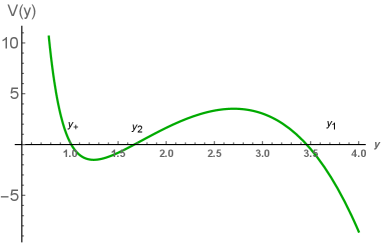
where $y_{1}$ and $y_{2}$ are given by (3.15). Therefore, there exists a pulsating string configuration, expanding and contracting between the turning points $\,y_{1}$ and $\,y_{2}\,$ . In Fig. 1 we plot the potential of the effective mechanical system (3.17). One can see that it has three positive real zeroes $y_{+}$ , $y_{1}$ , $y_{2}$ . The evolution of the pulsating string is defined in the region $\,y_{1}<y(\tau)<\,y_{2}\,$ .

We also note that $\Phi$ and $\Psi$ are defined by the relations

\Phi=m_{\phi}\sigma,\quad\Psi=m_{\psi}\sigma.

(3.19)

3.2 Pulsating string configuration on the subspace $y=const$

In order to obtain pulsating string solutions on the subspace $y=const$ we consider the following string ansatz ( $\,\kappa>0\,$ ):

T=\kappa\tau,\quad\Theta=\theta(\tau),\quad{\Phi=m_{\phi}\sigma+\phi(\tau),\quad\Psi=m_{\psi}\sigma+\psi(\tau)},\quad y=const.

(3.20)

Taking into account (3.20) the string Lagrangian can be represented as

	$\displaystyle\mathcal{L}_{P}$	$\displaystyle\sim$	$\displaystyle-\left(\kappa^{2}G_{TT}+\dot{\theta}^{2}G_{\Theta\Theta}+\dot{\phi}^{2}G_{\Phi\Phi}+\dot{\psi}^{2}G_{\Psi\Psi}+2\kappa(\dot{\phi}G_{T\Phi}+\dot{\psi}G_{T\Psi})+2\dot{\phi}\dot{\psi}G_{\Phi\Psi}\right)$		(3.21)
		$\displaystyle+$	$\displaystyle m_{\phi}^{2}G_{\Phi\Phi}+m_{\psi}^{2}G_{\Psi\Psi}+2m_{\phi}m_{\psi}G_{\Phi\Psi}.$		(3.21)

Let us list the relevant equations of motion (EoM). Since the ansatz (3.20) is linear in worldsheet time $\,\tau\,$ , the EoMs become actually equations with respect to $\,\sigma\,$ , while all constants $\,A_{T},\,\,A_{\phi},\,\,A_{\psi}\,$ below are the integration constants. The EoMs for $\,\Phi,\,\,\Psi\,$ and $\,T\,$ read off as follows

$\displaystyle\Phi:\quad$	$\displaystyle-$	$\displaystyle\frac{2M}{y^{2}\Xi^{3}}\kappa+\left(\frac{y^{2}}{a}+\frac{2aM}{y^{2}\Xi^{3}}\sin^{2}\theta\right)\dot{\phi}+\frac{2Ma\cos^{2}\theta}{\Xi^{3}y^{2}}\dot{\psi}=\frac{A_{\phi}}{a\sin^{2}\theta},$	(3.22)
$\displaystyle\Psi:\quad$	$\displaystyle-$	$\displaystyle\frac{2M}{y^{2}\Xi^{3}}\kappa+\left(\frac{y^{2}}{a}+\frac{2aM}{y^{2}\Xi^{3}}\cos^{2}\theta\right)\dot{\psi}+\frac{2Ma\sin^{2}\theta}{\Xi^{3}y^{2}}\dot{\phi}=\frac{A_{\psi}}{a\cos^{2}\theta},$	(3.23)
$\displaystyle T:\quad$		$\displaystyle\frac{2M}{y^{2}\Xi^{3}}\kappa-\frac{2aM}{y^{2}\Xi^{3}}(\dot{\phi}\sin^{2}\theta+\dot{\psi}\cos^{2}\Theta)=A_{T}+(1+y^{2}l^{2})\kappa.$	(3.24)

Correspondingly, the equation for $\,y\,$ has the form

	$\displaystyle\kappa^{2}(2\ell^{2}y+\frac{4M}{y^{3}\Xi^{3}})-2y\dot{\theta}^{2}-\frac{4\kappa}{y}\left(\frac{2Ma\sin^{2}\theta\dot{\phi}}{y^{2}\Xi^{3}}+\frac{2Ma\cos^{2}\theta\dot{\psi}}{y^{2}\Xi^{3}}\right)$	(3.25)
$\displaystyle+$	$\displaystyle 2y\left(\sin^{2}\theta m^{2}_{\phi}+m^{2}_{\psi}\cos^{2}\theta\right)-2y(\sin^{2}\theta\dot{\phi}^{2}+\cos^{2}\theta\dot{\psi}^{2})$
$\displaystyle-$	$\displaystyle\frac{4Ma^{2}}{y^{3}\Xi^{3}}\Bigl{(}-\sin^{4}\theta\dot{\phi}^{2}-\cos^{4}\theta\dot{\psi}^{2}-2\sin^{2}\theta\cos^{2}\theta\dot{\phi}\dot{\psi}$
$\displaystyle+$	$\displaystyle m^{2}_{\phi}\sin^{4}\theta+m^{2}_{\psi}\cos^{4}\theta+2m_{\phi}m_{\psi}\cos^{2}\theta\sin^{2}\theta\Bigr{)}=0.$

The equation for $T$ gives the ratio

\dot{\phi}\sin^{2}\theta+\dot{\psi}\cos^{2}\theta=\frac{y^{2}\Xi^{3}}{2aM}\left(\frac{2M}{y^{2}\Xi^{3}}\kappa-A_{T}-(1+y^{2}\ell^{2})\kappa\right).

(3.26)

Combining the equations for $\Phi\,$ , $\Psi\,$ and $T$ and doing some algebra we obtain the relevant equations for $\,\phi\,$ and $\,\psi\,$

$\displaystyle T+\Phi:$	$\displaystyle-$	$\displaystyle(1+y^{2}l^{2})\kappa+\frac{y^{2}}{a}\dot{\phi}=\frac{A_{\phi}}{a\sin^{2}\theta}+A_{T},$
$\displaystyle\dot{\phi}$	$\displaystyle=$	$\displaystyle\frac{1}{y^{2}}\frac{A_{\phi}}{\sin^{2}\theta}+\frac{a}{y^{2}}\left(A_{T}+(1+y^{2}\ell^{2})\kappa\right),$	(3.27)
$\displaystyle T+\Psi:$	$\displaystyle-$	$\displaystyle(1+y^{2}l^{2})\kappa+\frac{y^{2}}{a}\dot{\psi}=\frac{A_{\psi}}{a\sin^{2}\theta}+A_{T},$
$\displaystyle\dot{\psi}$	$\displaystyle=$	$\displaystyle\frac{1}{y^{2}}\frac{A_{\psi}}{\cos^{2}\theta}+\frac{a}{y^{2}}\left(A_{T}+(1+y^{2}\ell^{2})\kappa\right).$	(3.28)

Putting the expressions (3.27) and (3.28) into the equation for $T$ (3.26) we obtain the relation between constants

\frac{2M}{y^{2}\Xi^{3}}\kappa-\left(A_{\phi}+A_{\psi}\right)\frac{2aM}{y^{4}\Xi^{3}}-(1+\frac{2a^{2}M}{y^{4}\Xi^{3}})\left(A_{T}+(1+y^{2}\ell^{2})\kappa\right)=0.

(3.29)

The equations for the functions $\,\phi\,$ and $\,\psi\,$ can be rewritten in the form

	$\displaystyle\dot{\phi}$	$\displaystyle=$	$\displaystyle\frac{A_{\phi}}{y^{2}\sin^{2}\theta}+P-\frac{1}{y^{2}}(A_{\phi}+A_{\psi}),$		(3.30)
	$\displaystyle\dot{\psi}$	$\displaystyle=$	$\displaystyle\frac{A_{\psi}}{y^{2}\cos^{2}\theta}+P-\frac{1}{y^{2}}(A_{\phi}+A_{\psi}),$		(3.31)

where the constant $P$ is given by

P=\frac{1}{y^{2}}A_{\phi}+\frac{1}{y^{2}}A_{\psi}+\frac{a}{y^{2}}\left(A_{T}+(1+y^{2}\ell^{2})\kappa\right).

(3.32)

From here we find

\dot{\phi}\sin^{2}\theta+\dot{\psi}\cos^{2}\theta=P,\quad A_{T}+(1+y^{2}\ell^{2})\kappa=-\frac{2M(a(A_{\phi}+A_{\psi})-\kappa y^{2})}{2a^{2}M+y^{4}\Xi^{3}}.

(3.33)

Substituting (3.26) in (3.25) with $\frac{1}{y}$ factor we obtain the $y$ -equation in the form

	$\displaystyle\frac{\kappa^{2}}{y}\left(\ell^{2}y+\frac{2M}{y^{3}\Xi^{3}}\right)-\dot{\theta}^{2}-\frac{2\kappa}{y^{2}}\left(\frac{2M\kappa}{y^{2}\Xi^{3}}-(A_{T}+(1+y^{2}\ell^{2})\kappa)\right)$	(3.34)
$\displaystyle+$	$\displaystyle\left(\sin^{2}\theta m^{2}_{\phi}+m^{2}_{\psi}\cos^{2}\theta\right)-(\sin^{2}\theta\dot{\phi}^{2}+\cos^{2}\theta\dot{\psi}^{2})$
$\displaystyle-$	$\displaystyle\frac{2Ma^{2}}{y^{4}\Xi^{3}}\left(-(\sin^{2}\theta\dot{\phi}+\cos^{2}\theta\dot{\psi})^{2}+(m_{\phi}\sin^{2}\theta+m_{\psi}\cos^{2}\theta)^{2}\right)=0.$

The first Virasoro constraint (3.3) explicitly reads

			$\displaystyle-\frac{\kappa^{2}}{y^{2}}\left(1+y^{2}l^{2}-\frac{2M}{y^{2}\Xi^{3}}\right)-\frac{4aM}{y^{4}\Xi^{3}}\kappa(\sin^{2}\theta\dot{\phi}+\cos^{2}\theta\dot{\psi})+\dot{\theta}^{2}$		(3.35)
			$\displaystyle+(\sin^{2}\theta\dot{\phi}^{2}+\cos^{2}\theta\dot{\psi}^{2})+(\sin^{2}\theta m_{\phi}^{2}+\cos^{2}\theta m^{2}_{\psi})$
			$\displaystyle+2\frac{Ma^{2}}{\Xi^{3}y^{4}}\left((\sin^{2}\theta\dot{\phi}+\cos^{2}\theta\dot{\psi})^{2}+(\sin^{2}\theta m_{\phi}+\cos^{2}\theta m_{\psi})^{2}\right)=0.$

Remembering the equation for $\,y\,$ (3.34) and expression for the constant $\,P\,$ (3.32) and summing equations (3.34) and (3.35) we obtain the constraint

\displaystyle-\frac{\kappa^{2}}{y^{2}}+4\frac{\kappa^{2}M}{y^{4}\Xi^{3}}-8\frac{aM}{y^{4}\Xi^{3}}\kappa P+2\left(m^{2}_{\phi}\sin^{2}\theta+m^{2}_{\psi}\cos^{2}\theta\right)+\frac{4Ma^{2}}{y^{4}\Xi^{3}}P^{2}=0.

(3.36)

Since, $\,\theta\,$ is essentially time dependent (3.20), we are forward to impose the condition

m^{2}_{\phi}\,=\,m^{2}_{\psi}\,\equiv\,m^{2}.

(3.37)

With this choice the second Virasoro constraint (3.4) give us the relation

\textrm{Vir2}:\qquad-\frac{2M}{y^{2}\Xi^{3}}\kappa+(A_{\phi}+A_{\psi})(\frac{1}{a}+\frac{2aM}{y^{4}\Xi^{3}})+(1+\frac{2a^{2}M}{y^{4}\Xi^{3}})\left(A_{T}+(1+y^{2}\ell^{2})\kappa\right)=0.

(3.38)

As a result, we find

\frac{A_{\phi}+A_{\psi}}{a}=0,\quad A_{\phi}=-A_{\psi}\,\equiv\,A\,.

(3.39)

Thus, the constant $P$ (3.32) can be rewritten as

P=\frac{a}{y^{2}}(A_{T}+(1+y^{2}\ell^{2})\kappa).

(3.40)

Consequently, by virtue of the above relations between the constants and expression for the second Virasoro constraint (3.38) we can fix $\,A_{T}\,$

A_{T}\,=\,\frac{2M\kappa\,y^{2}}{2a^{2}M+y^{4}\Xi^{3}}-(1+y^{2}\ell^{2})\kappa\,,\qquad P=\frac{2aM\kappa}{2a^{2}M+y^{4}\Xi^{3}}.

(3.41)

Having $m^{2}_{\phi}=m^{2}_{\psi}=m^{2}$ and with the assumptions (3.39), the equation for the first Virasoro constraint (3.35) takes the form

\dot{\theta}^{2}-\frac{\kappa^{2}}{y^{2}}(1+y^{2}l^{2}-\frac{2M}{y^{2}\Xi^{3}})-\frac{4aM}{y^{4}\Xi^{3}}\kappa P+(2\frac{Ma^{2}}{\Xi^{3}y^{4}}+1)(P^{2}+m^{2})+\frac{A^{2}}{y^{4}}\frac{1}{\sin^{2}\theta\cos^{2}\theta}=0.

(3.42)

Finally, plugging the expression for $P$ (3.40) we obtain the following differential equation for $\,\theta\,$

\dot{\theta}^{2}+\frac{A^{2}}{y^{4}}\frac{1}{\sin^{2}\theta\cos^{2}\theta}+\Upsilon=0,

(3.43)

where

\Upsilon=-\frac{\kappa^{2}}{y^{2}}(1+y^{2}l^{2}-\frac{2M}{y^{2}\Xi^{3}})+(2\frac{Ma^{2}}{\Xi^{3}y^{4}}+1)m^{2}-\frac{4a^{2}M^{2}\kappa^{2}}{y^{4}\Xi^{3}(2Ma^{2}+y^{4}\Xi^{3})}.

(3.44)

At this point, it is convenient to introduce a new variable $u$

u(\tau)\equiv\sin^{2}\theta(\tau)>0,\quad 0<u<1.

(3.45)

Then we have

\frac{\dot{u}^{2}}{2}+2|\Upsilon|u^{2}-2|\Upsilon|u+\frac{2A^{2}}{y^{4}}=0,\qquad\Upsilon<0.

(3.46)

The equation (3.46) can be written in the form

\frac{\dot{u}^{2}}{2}+V(u)=0,\quad V(u)=2|\Upsilon|u^{2}-2|\Upsilon|u+\frac{2A^{2}}{y^{4}}.

(3.47)

If $\frac{4A^{2}}{|\Upsilon|^{2}\,y^{4}}\,<1\,$ the potential $V(u)$ has two turning points $\,u_{1,2}=\frac{1}{2}\mp\frac{\sqrt{1-\frac{4A^{2}}{|\Upsilon|^{2}\,y^{4}}}}{2}\,$ symmetrical about the point of minimum of the potential $\,u=\dfrac{1}{2}\,$ and $\,V(u)\leq 0\,$ , for $\,0<u_{1}\leq\,u(\tau)\,\leq\,u_{2}<1\,$ . Therefore, the above equation

\dot{u}^{2}=-4|\Upsilon|u^{2}+4|\Upsilon|u-\frac{4A^{2}}{y^{4}}\equiv\,-2V(u)\geq 0

(3.48)

has a periodic solution between turning points $\,u_{1,2}\,$ . The periodic solution of the above equation is

u(\tau)=\frac{1}{2}+\sqrt{\frac{1}{4}-\frac{A^{2}}{|\Upsilon|y^{4}}}\sin(2\sqrt{|\Upsilon}|\tau).

(3.49)

It is a pulsating string solution moving between the turning points. Correspondingly, the dynamics on the angular variables $\Phi$ and $\Psi$ is defined by (3.30)-(3.31),which with the constraint (3.39) and (3.45) take the form

	$\displaystyle\dot{\phi}$	$\displaystyle=$	$\displaystyle\frac{A}{y^{2}u(\tau)}+\frac{2aM\kappa}{2a^{2}M+y^{4}\Xi^{3}},$		(3.50)
	$\displaystyle\dot{\psi}$	$\displaystyle=$	$\displaystyle-\frac{A}{y^{2}(1-u(\tau))}+\frac{2aM\kappa}{2a^{2}M+y^{4}\Xi^{3}}.$		(3.51)

4 Energy spectrum

In this section we will semi-classically quantize the pulsating string configuration in 5d Kerr-AdS geometry. The approach has been presented for the first time in [19]. We will calculate the corresponding energy spectra. First, we will relate a study of the string energy spectra to the Bohr-Sommerfeld problem. After this, we discuss the large energies (large quantum numbers) to find the first correction to the energy. Note, the energy spectra of the circular string in the AdS background are related to the anomalous dimensions of the CFT operators according to the AdS/CFT dictionary. However, for the case of the Kerr-AdS spacetime we cannot carry out this connection, but we are able to relate the energy spectra to the dispersion relations.

4.1 Bohr-Sommerfeld analysis in 5d Kerr-AdS

We consider a circular closed string in the 5d Kerr-AdS black hole (2). In this analysis the string dynamics is governed by the Nambu-Goto action reads as

S_{NG}=-\frac{1}{2\pi\alpha^{\prime}}\int d\tau d\sigma\sqrt{|h|},

(4.1)

where the induced metric on the worldsheet

h_{\alpha\beta}=G_{MN}\partial_{\alpha}X^{M}\partial_{\beta}X^{N},\quad\textrm{with}\quad X^{M}=(T,\Theta,\Phi,\Psi,y)\,.

(4.2)

For the embedding we choose the ansatz

T=\kappa\,\tau,\qquad y=y(\tau),\qquad\Theta=\Theta^{*}\,=\,const,\qquad\Phi=\,m_{\phi}\sigma,\qquad\Psi=\,m_{\psi}\sigma\,.

(4.3)

The components of the induced metric (4.2) take the form

$\displaystyle h_{\tau\tau}$	$\displaystyle=$	$\displaystyle G_{TT}(\partial_{\tau}T)^{2}+G_{yy}(\partial_{\tau}y)^{2}=\kappa^{2}\Bigl{(}-1-y^{2}\ell^{2}+\frac{2M}{y^{2}\Xi^{3}}\Bigr{)}+\frac{\dot{y}_{\tau}^{2}}{f(y)},$	(4.4)
$\displaystyle h_{\sigma\sigma}$	$\displaystyle=$	$\displaystyle G_{\Phi\Phi}(\partial_{\sigma}\Phi)^{2}+2G_{\Phi\Psi}\partial_{\sigma}\Phi\partial_{\sigma}\Psi+G_{\Psi\Psi}(\partial_{\sigma}\Psi)^{2}$	(4.5)
	$\displaystyle=$	$\displaystyle y^{2}(\sin^{2}\Theta^{}m^{2}_{\phi}+\cos^{2}\Theta^{}m_{\psi}^{2})+\frac{2Ma^{2}}{\Xi^{3}y^{2}}\left(\sin^{2}\Theta^{}{}m_{\phi}+\cos^{2}\Theta^{}m_{\psi}\right)^{2},$	(4.5)
$\displaystyle h_{\sigma\tau}$	$\displaystyle=$	$\displaystyle 2G_{T\Phi}\partial_{\tau}T\partial_{\sigma}\Phi+2G_{T\Psi}\partial_{\tau}T\partial_{\sigma}\Psi=-\frac{2\kappa Ma}{\Xi^{3}y^{2}}\Bigr{(}\sin^{2}\Theta^{}m_{\phi}+\cos^{2}\Theta^{}m_{\psi}\Bigr{)}.$	(4.6)

By virtue of (4.4)-(4.6) the NG action (4.1) is written down as

S_{NG}=-\frac{1}{2\pi\alpha^{\prime}}\int d\tau d\sigma\sqrt{\Bigr{(}\kappa^{2}\Bigl{(}1+y^{2}\ell^{2}-\frac{2M}{y^{2}\Xi^{3}}\Bigr{)}-\frac{\dot{y}_{\tau}^{2}}{f(y)}\Bigr{)}\cdot\Bigr{(}y^{2}\tilde{\mathcal{M}}+\frac{2Ma^{2}}{\Xi^{3}y^{2}}\mathcal{M}^{2}\Bigr{)}+\Bigr{(}\frac{2\kappa Ma}{\Xi^{3}y^{2}}\mathcal{M}\Bigr{)}^{2}},

(4.7)

where

f(y)=1+\frac{2Ma^{2}}{\Xi^{3}y^{4}}-\frac{2M}{\Xi^{2}y^{2}}+\ell^{2}y^{2}

(4.8)

and

\mathcal{M}=m_{\phi}\sin^{2}\Theta^{*}+m_{\psi}\cos^{2}\Theta^{*},\quad\tilde{\mathcal{M}}=m^{2}_{\phi}\sin^{2}\Theta^{*}+m^{2}_{\psi}\cos^{2}\Theta^{*}.

(4.9)

Doing some algebra, we can be represent the action (4.7) in the simplified form

S_{NG}=-\frac{1}{2\pi\alpha^{\prime}}\frac{\kappa}{\Xi^{3/2}}\int d\tau\sqrt{(1+\ell^{2}y^{2})\left(y^{2}\Xi^{3}\tilde{\mathcal{M}}+\frac{2M\mathcal{M}^{2}a^{2}}{y^{2}}\right)-2M\tilde{\mathcal{M}}-\frac{\dot{y}^{2}_{\tau}}{\kappa^{2}f(y)}\left(y^{2}\Xi^{3}\tilde{\mathcal{M}}+\frac{2M\mathcal{M}^{2}a^{2}}{y^{2}}\right)}.

(4.10)

The canonical momentum corresponding to (4.7) is

\Pi=-\frac{\dot{y}(2a^{2}M\mathcal{M}^{2}+\tilde{\mathcal{M}}\Xi^{3}y^{4})}{\kappa\Xi^{3/2}yf(y)\sqrt{(1+\ell^{2}y^{2})(2a^{2}M\mathcal{M}^{2}+\tilde{\mathcal{M}}\Xi^{3}y^{4})-2M\tilde{\mathcal{M}}y^{2}-\frac{\dot{y}^{2}\left(2a^{2}M\mathcal{M}^{2}+\tilde{\mathcal{M}}\Xi^{3}y^{4}\right)}{\kappa^{2}f(y)}}}.

(4.11)

and the first integral related to (4.7) is given by

\mathcal{H}=-\frac{\kappa\left((\tilde{\mathcal{M}}\Xi^{3}y^{4}+2a^{2}M\mathcal{M}^{2})(1+\ell^{2}y^{2})-2M\tilde{\mathcal{M}}y^{2}\right)}{\Xi^{3/2}y\sqrt{(1+\ell^{2}y^{2})(2a^{2}M\mathcal{M}^{2}+\tilde{\mathcal{M}}\Xi^{3}y^{4})-2M\tilde{\mathcal{M}}y^{2}-\frac{\dot{y}^{2}\left(2a^{2}M\mathcal{M}^{2}+\tilde{\mathcal{M}}\Xi^{3}y^{4}\right)}{f(y)\kappa^{2}}}}.

(4.12)

It is convenient to pass to a new variable³³3Comment on the change of the variable $\xi=\int\mathbf{f}(y)dy$ $\Rightarrow$ $\xi=\mathbf{F}(y)$ $\Rightarrow$ $\xi=\mathbf{F}(y(\tau))$ $\Rightarrow$ $\dot{\xi}=\frac{\partial\mathbf{F}}{\partial y}\dot{y}$ $\Rightarrow$ $\xi=\mathbf{f}(y)\dot{y}$ .

\xi=\int\frac{dy}{\sqrt{\kappa f(y)}}\sqrt{\frac{(y^{2}\Xi^{3}\tilde{\mathcal{M}}+\frac{2M\mathcal{M}^{2}a^{2}}{y^{2}})}{(1+\ell^{2}y^{2})(y^{2}\Xi^{3}\tilde{\mathcal{M}}+\frac{2M\mathcal{M}^{2}a^{2}}{y^{2}})-2M\tilde{\mathcal{M}}}}.

(4.13)

In terms of the $\xi$ -variable (4.13) the string Lagrangian (4.7) significantly simplifies

L_{s}\sim\frac{g(\xi)}{\Xi^{3/2}}\sqrt{1-\dot{\xi}^{2}},

(4.14)

where the function $g(\xi)$ is defined as

g(\xi)=\sqrt{(1+\ell^{2}y^{2})\Bigl{(}y^{2}\Xi^{3}\tilde{\mathcal{M}}+\frac{2M\mathcal{M}^{2}a^{2}}{y^{2}}\Bigr{)}-2M\tilde{\mathcal{M}}}.

(4.15)

The Hamiltonian and the canonical momenta take the form, correspondingly

\mathcal{H}_{\xi}=-\frac{g(\xi)}{\Xi^{3/2}\sqrt{1-\dot{\xi}^{2}}},\quad\Pi_{\xi}=-\frac{g(\xi)\dot{\xi}}{\Xi^{3/2}\sqrt{1-\dot{\xi}^{2}}}

(4.16)

Then the system can be described as

\mathcal{H}_{\xi}=\sqrt{\Pi^{2}_{\xi}+V_{\xi}},

(4.17)

where the potential is given by

V_{\xi}=\frac{g(\xi)^{2}}{\Xi^{3}}.

(4.18)

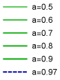
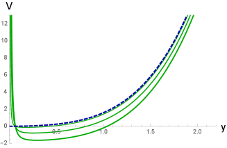
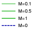
The behaviour of the potential $V$ (4.18) is presented in Fig. 2. In Fig. 2 a) and b) we show the potential for the fixed mass of the black hole varying the rotational parameter, the case a) corresponds to a small rotational parameter, while b) is for $a\in(0.5;0.97)$ . We recall that $a=1$ is a critical value of the rotational parameter for $\ell=1$ . In Fig. 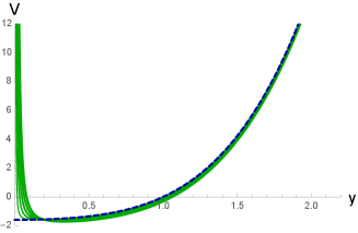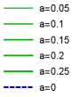2 b) we observe a jump of the potential for $a=0.97$ .

The horizon of the black hole $y_{+}$ and the boundary of the background can be considered as potential wells. So we can perform the Bohr-Sommerfeld analysis for the quantization. Then we have the following condition

(n+\frac{1}{2})\pi=\int^{\xi_{2}}_{\xi_{1}}d\xi\sqrt{E^{2}-\frac{g(\xi)^{2}}{\alpha^{\prime 2}\Xi^{3}}},

(4.19)

with the turning point $\xi_{1,2}$ .

In terms of the holographic radial coordinate $y$ (4.19) takes the form

	$\displaystyle\left(n+\frac{1}{2}\right)\pi=\int^{y_{1}}_{y_{+}}\frac{Edy}{\sqrt{\kappa f(y)}}\sqrt{\frac{(y^{2}\Xi^{3}\tilde{\mathcal{M}}+\frac{2M\mathcal{M}^{2}a^{2}}{y^{2}})}{(1+\ell^{2}y^{2})(y^{2}\Xi^{3}\tilde{\mathcal{M}}+\frac{2M\mathcal{M}^{2}a^{2}}{y^{2}})-2M\tilde{\mathcal{M}}}}\times$
	$\displaystyle\sqrt{1-\frac{(1+\ell^{2}y^{2})\Bigl{(}y^{2}\Xi^{3}\tilde{\mathcal{M}}+\frac{2M\mathcal{M}^{2}a^{2}}{y^{2}}\Bigr{)}-2M\tilde{\mathcal{M}}}{\alpha^{\prime 2}\Xi^{3}E^{2}}}$
	$\displaystyle=E\int^{y_{1}}_{y_{+}}dy\sqrt{Q(y)}\left(\frac{1}{\sqrt{\kappa f(y)}\sqrt{P(y)}}-\frac{1-\sqrt{1-\frac{1}{B^{2}\Xi^{3}\tilde{\mathcal{M}}}P(y)}}{\sqrt{\kappa f(y)}\sqrt{P(y)}}\right),$		(4.20)

where we define $B=\frac{E\alpha^{\prime}}{\sqrt{\tilde{\mathcal{M}}}}$ and

	$\displaystyle P(y)$	$\displaystyle=$	$\displaystyle(1+\ell^{2}y^{2})\left(y^{2}\Xi^{3}\tilde{\mathcal{M}}+\frac{2M\mathcal{M}^{2}a^{2}}{y^{2}}\right)-2M\tilde{\mathcal{M}},$		(4.21)
	$\displaystyle Q(y)$	$\displaystyle=$	$\displaystyle y^{2}\Xi^{3}\tilde{\mathcal{M}}+\frac{2M\mathcal{M}^{2}a^{2}}{y^{2}}.$		(4.22)

We are not able to calculate eq. (4.20) exactly. However, supposing that the rotational parameter $a$ is small we can expand in series (4.20), then we get

	$\displaystyle\left(n+\frac{1}{2}\right)\pi=\frac{E}{\sqrt{\kappa}}\int^{\tilde{y}_{1}}_{y_{H}}dy\left(\frac{1}{1-\frac{2M}{y^{2}}+\ell^{2}y^{2}}-\frac{1-\sqrt{1-\frac{y^{2}}{B^{2}}(1+\ell^{2}y^{2}-\frac{2M}{y^{2}})}}{1-\frac{2M}{y^{2}}+\ell^{2}y^{2}}\right)+$		(4.23)
	$\displaystyle\frac{2\tilde{\mathcal{M}}y^{2}((5\ell^{2}y^{2}-1)-\frac{y^{2}}{B^{2}}(2\ell^{2}y^{2}-1)(1+\ell^{2}y^{2}-\frac{2M}{y^{2}}))-3\mathcal{M}^{2}(2M+\frac{y^{4}}{B^{2}}(1+\ell^{2}y^{2}-\frac{2M}{y^{2}})^{2})}{2\sqrt{\kappa}\tilde{\mathcal{M}}y^{6}(\ell^{2}y^{2}-\frac{2M}{y^{2}}+1)^{2}\sqrt{1-\frac{y^{2}}{B^{2}}(\ell^{2}y^{2}+1-\frac{2M}{y^{2}})}}a^{2}M.$

In eq. (4.23) we observe the contribution

h(y)=1-\frac{2M}{y^{2}}+\ell^{2}y^{2},

(4.24)

which is nothing but the blackenning function of the AdS-Schwarzschild black hole, i.e. the black hole without rotation. The horizon $y_{H}$ for the the AdS-Schwarzschild black hole is defined as a root of the equation $h(y)=0$ , i.e.

y_{H}=\frac{1}{\ell}\sqrt{\frac{1}{2}\Bigr{(}1+\sqrt{1+8M\ell^{2}}\Bigr{)}}.

(4.25)

It is worth to note that the quantities $h(y)$ (4.24) and $y_{H}$ (4.25) related to the non-rotating AdS black hole appear due to expanding around a small rotational parameter $a$ .

Integrating the first term in the integral (4.23) we get

	$\displaystyle\frac{E}{\sqrt{\kappa}}\int^{\tilde{y}_{1}}_{y_{H}}dy\frac{1}{1-\frac{2M}{y^{2}}+\ell^{2}y^{2}}=-\frac{E}{\sqrt{\kappa}}\frac{\sqrt{\sqrt{1+8\ell^{2}M}-1}\tanh^{-1}\left(\frac{\sqrt{2}\ell y}{\sqrt{\sqrt{1+8\ell^{2}M}-1}}\right)}{\ell\sqrt{2}\sqrt{1+8\ell^{2}M}}\Big{\|}^{\tilde{y}_{1}}_{y_{H}}$		(4.26)
	$\displaystyle+\frac{E}{\sqrt{\kappa}}\frac{2\sqrt{M}\tan^{-1}\left(\frac{\sqrt{2}\ell y}{\sqrt{\sqrt{1+8\ell^{2}M}+1}}\right)}{\sqrt{1+8\ell^{2}M}\sqrt{\sqrt{1+8\ell^{2}M}-1}}\Big{\|}^{\tilde{y}_{1}}_{y_{H}}.$

In the case of large energies $B\cdot\ell\gg 1$ eq.(4.26) can be approximated as follows

\int^{\tilde{y}_{1}}_{y_{H}}dy\frac{1}{1-\frac{2M}{y^{2}}+\ell^{2}y^{2}}\approx\frac{\pi}{2}\sqrt{\frac{1}{\sqrt{2M}\ell^{3}}}-\sqrt{\frac{1}{B\ell^{3}}}.

(4.27)

The second integral (4.1) can be calculated easily in terms of a new variable $y=r\sqrt{B/\ell}$

	$\displaystyle\int^{y_{1}}_{y_{H}}dy\frac{1-\sqrt{1-\frac{y^{2}}{B^{2}}\left(1+\ell^{2}y^{2}-\frac{2M}{y^{2}}\right)}}{1+y^{2}\ell^{2}-\frac{2M}{y^{2}}}$	$\displaystyle\rightarrow$	$\displaystyle\sqrt{\frac{1}{\ell^{3}B}}\int^{1}_{0}\frac{dr}{r^{2}}(1-\sqrt{1-r^{4}})$		(4.28)
		$\displaystyle=$	$\displaystyle\sqrt{\frac{1}{\ell^{3}B}}\left(-1+\frac{(2\pi)^{3/2}}{\Gamma(\frac{1}{4})^{2}}\right).$		(4.28)

Applying the same procedure to the third integral (4.1), in the limit of large $B$ we get

	$\displaystyle\int^{\tilde{y}}_{y_{+}}dy\frac{2\tilde{\mathcal{M}}y^{2}((5\ell^{2}y^{2}-1)-\frac{y^{2}}{B^{2}}(2\ell^{2}y^{2}-1)(1+\ell^{2}y^{2}-\frac{2M}{y^{2}}))-3\mathcal{M}^{2}(2M+\frac{y^{4}}{B^{2}}(1+\ell^{2}y^{2}-\frac{2M}{y^{2}})^{2})}{2\tilde{\mathcal{M}}y^{6}(\ell^{2}y^{2}-\frac{2M}{y^{2}}+1)^{2}\sqrt{1-\frac{y^{2}}{B^{2}}(\ell^{2}y^{2}+1-\frac{2M}{y^{2}})}}a^{2}M$	(4.29)
$\displaystyle=$	$\displaystyle-\frac{\sqrt{\ell}}{B^{5/2}}Ma^{2}\int^{1}_{0}dr\left(\frac{2}{r^{2}\sqrt{1-r^{4}}}-\frac{5}{r^{6}\sqrt{1-r^{4}}}+\frac{3\mathcal{M}^{2}}{2\tilde{\mathcal{M}}r^{2}\sqrt{1-r^{4}}}\right)$
$\displaystyle=$	$\displaystyle-\frac{\sqrt{\ell}}{B^{5/2}}\left(\frac{\sqrt{2}\pi^{3/2}}{\Gamma(\frac{1}{4})^{2}}+\frac{3\sqrt{\pi}\mathcal{M}^{2}\Gamma(\frac{3}{4})}{2\tilde{\mathcal{M}}\Gamma(\frac{1}{4})}\right)Ma^{2}.$

Combining together (4.27),(4.28) and (4.29) we get for Bohr-Sommerfeld quantisation condition

(n+\frac{1}{2})\pi\approx\frac{1}{\ell^{3/2}\sqrt{\kappa}}\left(\frac{\pi}{2}\frac{E}{(\sqrt{2M})^{1/2}}-\frac{(2\pi)^{3/2}}{\Gamma(\frac{1}{4})^{2}}\frac{(\tilde{\mathcal{M}}E)^{1/2}}{(\alpha^{\prime})^{1/2}}-\frac{\ell^{2}\sqrt{\pi}\tilde{\mathcal{M}}^{5/4}}{\alpha^{5/2}E^{3/2}}\left(\frac{\sqrt{2}\pi}{\Gamma(\frac{1}{4})^{2}}+\frac{3\mathcal{M}^{2}\Gamma(\frac{3}{4})}{2\tilde{\mathcal{M}}\Gamma(\frac{1}{4})}\right)Ma^{2}\right).

(4.30)

In (4.30) we can recognize the result for the energy from [12] if one sends $a$ to $0$ .

4.2 WKB approximation

4.2.1 Derivation of the Hamiltonian

As in the previous section the string dynamics is governed by the Nambu-Goto action (4.1) with the induced metric (4.2). The first ingredient towards finding the spectrum is to make a pullback of the line element of the metric of the 5d Kerr-AdS background (2) to the subspace, where string dynamics takes place. In this section one can consider more general ansatz than (3.20) and (4.3), such as

		$\displaystyle\Theta\equiv\,\xi_{1}=\xi_{1}(\tau)\,,\,y\equiv\,\xi_{2}=\xi_{2}(\tau)\,,$		(4.31)
		$\displaystyle T\equiv\,X_{0}=x_{0}(\tau)+m_{0}\sigma,\qquad x_{0}(\tau)=\kappa\tau,\qquad m_{0}=0\,,$		(4.32)
		$\displaystyle\Phi\equiv\,X_{1}=m_{1}\sigma+x_{1}(\tau)\,,\quad\Psi\equiv\,X_{2}=m_{2}\sigma+x_{2}(\tau)\,.$		(4.33)

For convenience, we use the following notations of the Kerr-AdS metric (2)

ds^{2}=\sum\limits_{i,j=1}^{2}g_{ij}d\xi_{i}d\xi_{j}\,+\,\sum\limits_{k,p=0}^{2}\hat{G}_{kp}dX_{k}dX_{p}\,,

(4.34)

where the following quantities have been defined

\left(g_{ij}\right)=\left(\begin{matrix}G_{\Theta\Theta}&0\\ 0&G_{yy}\end{matrix}\right)\,,\qquad i,j=1,2\,,

(4.35)

\left(\hat{G}_{kp}\right)=\left(\begin{matrix}G_{TT}&G_{T\Phi}&G_{T\Psi}\\ G_{T\Phi}&G_{\Phi\Phi}&G_{\Phi\Psi}\\ G_{T\Psi}&G_{\Phi\Psi}&G_{\Psi\Psi}\end{matrix}\right)\,,\qquad k,p=0,1,2\,,

(4.36)

and the submatrix

\left(\hat{g}_{kp}\right)=\left(\begin{matrix}G_{\Phi\Phi}&G_{\Phi\Psi}\\ G_{\Phi\Psi}&G_{\Psi\Psi}\end{matrix}\right)\,,\qquad k,p=1,2\,.

(4.37)

We note, that for the inverse of $\left(\hat{g}_{kp}\right)$ matrix, we find

\left(\hat{g}^{kp}\right)=\left(\begin{matrix}\frac{y^{4}\Xi^{3}+2a^{2}M\cos^{2}\Theta}{y^{2}\sin^{2}\Theta\,(y^{4}\Xi^{3}+2a^{2}M)}&-\,\frac{2a^{2}M}{y^{2}\,(y^{4}\Xi^{3}+2a^{2}M)}\\ -\,\frac{2a^{2}M}{y^{2}\,(y^{4}\Xi^{3}+2a^{2}M)}&\frac{y^{4}\Xi^{3}+2a^{2}M\sin^{2}\Theta}{y^{2}\cos^{2}\Theta\,(y^{4}\Xi^{3}+2a^{2}M)}\end{matrix}\right)\,,\qquad k,p=1,2\,.

(4.38)

The components of the induced metric on the worldsheet:

ds^{2}_{ws}=\left(\sum\limits_{i,j=1}^{2}g_{ij}\,\dot{\xi}_{i}\dot{\xi}_{j}+\sum\limits_{k,p=0}^{2}\hat{G}_{kp}\,\dot{x}_{k}\dot{x}_{p}\right)d\tau^{2}+\left(\sum\limits_{k,p=0}^{2}\hat{G}_{kp}\,m_{k}m_{p}\right)\,d\sigma^{2}+\\ +2\left(\sum\limits_{k,p=0}^{2}\hat{G}_{kp}\,m_{k}\dot{x}_{p}\right)\,d\tau d\sigma\,.

(4.39)

The Nambu-Goto action (4.1) with (4.2) becomes

S_{NG}=-\,\dfrac{1}{\alpha^{\prime}}\int\,d\tau\,\sqrt{\left(\sum\limits_{k,p=1}^{2}\hat{G}_{kp}\,m_{k}\dot{x}_{p}+\sum\limits_{k=1}^{2}\hat{G}_{k0}\,m_{k}\,\kappa\right)^{2}+\,\,}\\ \overline{\,\,-\left\|\vec{m}\right\|^{2}\,\left(\sum\limits_{i,j=1}^{2}g_{ij}\,\dot{\xi}_{i}\dot{\xi}_{j}+\sum\limits_{k,p=1}^{2}\hat{g}_{kp}\,\dot{x}_{k}\dot{x}_{p}+\hat{G}_{00}\,\kappa^{2}+2\,\sum\limits_{k=1}^{2}\hat{G}_{0k}\,\kappa\dot{x}_{k}\right)\,\,}\,,

(4.40)

where $1/\alpha^{\prime}=\sqrt{\lambda}$ is the ’t Hooft coupling constant and

\displaystyle\left\|\vec{m}\right\|^{2}=\sum\limits_{k,h=0}^{2}\hat{G}_{kh}m_{k}m_{h}=\sum\limits_{k,h=1}^{2}\hat{G}_{kh}(\xi_{1},\xi_{2})m_{k}m_{h}\equiv\sum\limits_{k,h=1}^{2}\hat{g}_{kh}(\xi_{1},\xi_{2})m_{k}m_{h}\,>\,0\,.

(4.41)

The problem reduces again to the dynamics of an effective point-particle with Lagrangian

L_{eff}=-\,\sqrt{\lambda}\,\sqrt{\left(\sum\limits_{k,p=1}^{2}\hat{g}_{kp}\,m_{k}\dot{x}_{p}+\sum\limits_{k=1}^{2}\hat{G}_{k0}\,m_{k}\,\kappa\right)^{2}-\left\|\vec{m}\right\|^{2}\,\left(\sum\limits_{i,j=1}^{2}g_{ij}\,\dot{\xi}_{i}\dot{\xi}_{j}+\,\,\right.}\\ \overline{\left.\,\,+\sum\limits_{k,p=1}^{2}\hat{g}_{kp}\,\dot{x}_{k}\dot{x}_{p}+\hat{G}_{00}\,\kappa^{2}+2\,\sum\limits_{k=1}^{2}\hat{G}_{0k}\,\kappa\dot{x}_{k}\right)\,\,}\,.

(4.42)

For convenience we will use the shorthand notation

\sqrt{\left(\sum\limits_{k,p=1}^{2}\hat{g}_{kp}\,m_{k}\dot{x}_{p}+\sum\limits_{k=1}^{2}\hat{G}_{k0}\,m_{k}\,\kappa\right)^{2}-\left\|\vec{m}\right\|^{2}\,\left(\sum\limits_{i,j=1}^{2}g_{ij}\,\dot{\xi}_{i}\dot{\xi}_{j}+\,\,\right.}\\ \overline{\left.\,\,+\sum\limits_{k,p=1}^{2}\hat{g}_{kp}\,\dot{x}_{k}\dot{x}_{p}+\hat{G}_{00}\,\kappa^{2}+2\,\sum\limits_{k=1}^{2}\hat{G}_{0k}\,\kappa\dot{x}_{k}\right)\,\,}\,\equiv\,\sqrt{......\,\,}\,.

(4.43)

As before, it is useful to consider the Hamiltonian formulation of the problem. To this end, we have to calculate the canonical momenta

	$\displaystyle\Pi_{\xi_{i}}$	$\displaystyle=\frac{\partial L_{eff}}{\partial\dot{\xi}_{i}}=\sqrt{\lambda}\,\dfrac{\left\\|\vec{m}\right\\|^{2}g_{ij}\,\dot{\xi}_{j}}{\sqrt{......\,\,}}\,,$		(4.44)
	$\displaystyle\Pi_{x_{p}}$	$\displaystyle=\frac{\partial L_{eff}}{\partial\dot{x}_{p}}=\sqrt{\lambda}\,\dfrac{\,\left\\|\vec{m}\right\\|^{2}\hat{g}_{pq}\,\dot{x}_{q}-(\hat{g}_{kq}\,m_{k}\dot{x}_{q})\,\hat{g}_{pq}\,m_{q}+\left\\|\vec{m}\right\\|^{2}\hat{G}_{p0}\,\kappa-(\hat{G}_{k0}\,m_{k}\kappa)\,\hat{g}_{pq}\,m_{q}\,}{\sqrt{......\,\,}}\,,$		(4.45)

which also implies the constraint

\sum\limits_{p=1}^{2}m_{p}\,\Pi_{x_{p}}=0.

(4.46)

Applying a Legendre transformation, it is straightforward to find the (square of) the pulsating string Hamiltonian

H^{2}=\kappa^{2}\,\left(\sum\limits_{l,s=1}^{2}\hat{G}_{0l}\,\hat{g}^{ls}\,\Pi_{x_{s}}\right)^{2}+\\ -\kappa^{2}\,\left(\hat{G}_{00}+\sum\limits_{l,s=1}^{2}\hat{G}_{0l}\,\hat{g}^{ls}\,\hat{G}_{s0}\right)\,\left\{\sum\limits_{i,j=1}^{2}\Pi_{\xi_{i}}\,g^{ij}\,\Pi_{\xi_{j}}+\sum\limits_{i,j=1}^{2}\Pi_{x_{i}}\,\hat{g}^{ij}\,\Pi_{x_{j}}+\lambda\,\left\|\vec{m}\right\|^{2}\right\}\,.

(4.47)

The explicit expressions for the terms in the brackets are

\sum\limits_{l,s=1}^{2}\hat{G}_{0l}\,\hat{g}^{ls}\,\Pi_{x_{s}}\,=\,-\,h_{2}(y)\,\left(\Pi_{x_{1}}+\Pi_{x_{2}}\right)

(4.48)

and

\hat{G}_{00}+\sum\limits_{l,s=1}^{2}\hat{G}_{0l}\,\hat{g}^{ls}\,\hat{G}_{s0}\,=\,-\,\frac{y^{2}\Xi^{3}-2aM\,h_{1}(y)\,h_{2}(y)}{h_{1}(y)\,y^{2}\Xi^{3}}\,\equiv\,-\,K^{2}(y)\,,

(4.49)

where

h_{1}(y)\,=\,\frac{y^{2}\Xi^{3}}{-2M+y^{2}(1+\ell^{2}y^{2})\Xi^{3}}\,,\qquad h_{2}(y)\,=\,\frac{2aM}{2a^{2}M+y^{4}\Xi^{3}}\,.

(4.50)

The expression of $H^{2}$ can be conveniently written

\frac{H^{2}}{\kappa^{2}}\,=\,K^{2}(y)\left\{\sum\limits_{i,j=1}^{2}\Pi_{\xi_{i}}\,g^{ij}\,\Pi_{\xi_{j}}+\sum\limits_{i,j=1}^{2}\Pi_{x_{i}}\,\left[\frac{h_{2}^{2}(y)}{K^{2}(y)}\,\hat{\delta}^{ij}+\hat{g}^{ij}\right]\,\Pi_{x_{j}}+\lambda\,\left\|\vec{m}\right\|^{2}\right\}\,,

(4.51)

where

\left(\hat{\delta}^{ij}\right)\,=\,\left(\begin{matrix}1&1\\ 1&1\end{matrix}\right)\,,\,\,i,j=1,2\,.

(4.52)

It should be noted here that the above Hamiltonian (4.47) can be considered as the effective Hamiltonian of an effective point-particle on the Kerr-AdS background. The last term

-\lambda\,\kappa^{2}\,\left\|\vec{m}\right\|^{2}\,\left(\hat{G}_{00}+\sum\limits_{l,s=1}^{2}\hat{G}_{0l}\,\hat{g}^{ls}\,\hat{G}_{s0}\right)\,\equiv\,\lambda\,\kappa^{2}\,\left\|\vec{m}\right\|^{2}\,K^{2}(y)\,\equiv\,\lambda\,U(\Theta,\,y)\,,

(4.53)

serves as an effective potential, which encodes the relevant dynamics of the strings.
In the context of the holographic correspondence, the potential is very small comparing to the kinetic part. Therefore, we can calculate quantum corrections to the energy by making use of the perturbation theory.

4.2.2 Laplace-Beltrami operator and wave function

The standard Laplace-Beltrami operator in the AdS coordinates for the 5d Kerr-AdS (2) is

\bigtriangleup^{(5)}_{Kerr-AdS}\,=\,G^{TT}\frac{\partial^{2}}{\partial T^{2}}+2\,G^{T\Phi(\Psi)}\frac{\partial}{\partial T}\left(\frac{\partial}{\partial\Phi}+\frac{\partial}{\partial\Psi}\right)+G^{\Phi\Phi}\frac{\partial^{2}}{\partial\Phi^{2}}+2\,G^{\Phi\Psi}\frac{\partial^{2}}{\partial\Phi\partial\Psi}+G^{\Psi\Psi}\frac{\partial^{2}}{\partial\Psi^{2}}+\\ +\frac{1}{\sqrt{-\det G}}\,\frac{\partial}{\partial\Theta}\left(\sqrt{-\det G\,}\,G^{\Theta\Theta}\,\frac{\partial}{\partial\Theta}\right)++\frac{1}{\sqrt{-\det G}}\,\frac{\partial}{\partial y}\left(\sqrt{-\det G\,}\,G^{yy}\,\frac{\partial}{\partial y}\right)\,.

(4.54)

In the notations of Appendix A (see (A.1) and (A.5)), we have

\bigtriangleup^{(5)}_{Kerr-AdS}\,=\,-h_{1}(y)\,\frac{\partial^{2}}{\partial T^{2}}-2\,h_{1}(y)\,h_{2}(y)\,\frac{\partial}{\partial T}\left(\frac{\partial}{\partial\Phi}+\frac{\partial}{\partial\Psi}\right)+\\ -\,\frac{1}{y^{2}}a\,h_{2}(y)\,\left(\frac{\partial}{\partial\Phi}+\frac{\partial}{\partial\Psi}\right)^{2}+\frac{1}{y^{2}\sin^{2}\Theta}\,\frac{\partial^{2}}{\partial\Phi^{2}}+\frac{1}{y^{2}\cos^{2}\Theta}\,\frac{\partial^{2}}{\partial\Psi^{2}}+\\ +\frac{1}{y^{2}}\,\frac{1}{\sin(2\Theta)}\frac{\partial}{\partial\Theta}\left(\sin(2\Theta)\,\frac{\partial}{\partial\Theta}\right)+\frac{1}{\sqrt{h(y)\,}}\,\frac{\partial}{\partial y}\left(\sqrt{h(y)\,}\,G^{yy}\,\frac{\partial}{\partial y}\right)\,,

(4.55)

where $h_{1}(y)$ and $h_{2}(y)$ are given by (4.50).

To obtain the wave function, we have to solve the equation

\bigtriangleup^{(5)}_{Kerr-AdS}\,F(T,\,\Theta,\,y,\,\Phi,\,\Psi)\,=\,0\,,

(4.56)

using separation of variables

F(T,\,\Theta,\,y,\,\Phi,\,\Psi)\,=\,e^{-iE\,T}\,e^{in_{1}\Phi}\,e^{in_{2}\Psi}\,f(\Theta,\,y)\,,\qquad n_{1},\,n_{2}\,\in\mathbb{Z}\,.

(4.57)

Substituting (4.57) in to the equation (4.56), we find the following partial differential equation for $\,f(\Theta,\,y)\,$

E^{2}\,h_{1}(y)\,f-2h_{1}(y)h_{2}(y)\,E\,(n_{1}+n_{2})\,f+\frac{1}{y^{2}}\,ah_{2}(y)\,(n_{1}+n_{2})^{2}\,f+\\ -\frac{1}{y^{2}}\,\left(\frac{n_{1}^{2}}{\sin^{2}\Theta}+\frac{n_{2}^{2}}{\cos^{2}\Theta}\right)\,f+\frac{1}{y^{2}}\,\frac{1}{\sin(2\Theta)}\frac{\partial}{\partial\Theta}\left(\sin(2\Theta)\,\frac{\partial f}{\partial\Theta}\right)+\\ +\frac{1}{\sqrt{h(y)\,}}\,\frac{\partial}{\partial y}\left(\sqrt{h(y)\,}\,G^{yy}\,\frac{\partial f}{\partial y}\right)\,=\,0\,.

(4.58)

We can further separate the variables defining $\,f(\Theta,\,y)\,=\,f(\Theta)\,Y(y)\,$ .

4.2.3 Solving the Schrödinger equation on the reduced subspace $y=const$

In the subsection (3.2), we obtain an explicit pulsating solution (3.49) in the case for the string winding numbers satisfy $\,m_{1}^{2}=m_{2}^{2}\equiv\,m^{2}\,$ and $\,y=const\neq\,0\,$ .
In this case, taking into account (4.46), for the first term of the Hamiltonian (4.47), we have

\left(\sum\limits_{l,s=1}^{2}\hat{G}_{0l}\,\hat{g}^{ls}\,\Pi_{x_{s}}\right)^{2}\,=\,h^{2}_{2}(y)\,\left(\Pi_{x_{1}}+\Pi_{x_{2}}\right)^{2}\,=\,0\,.

(4.59)

Moreover, all functions of $y$ are constants and

\hat{G}_{00}+\sum\limits_{l,s=1}^{2}\hat{G}_{0l}\,\hat{g}^{ls}\,\hat{G}_{s0}\,=\,-\frac{y^{2}\Xi^{3}-2aM\,h_{1}(y)\,h_{2}(y)}{h_{1}(y)\,y^{2}\Xi^{3}}\,\equiv\,-K^{2}=const\,,

(4.60)

where $h_{1}$ and $h_{2}$ (4.50) are taken to be constant. Therefore, the square of the Hamiltonian (4.47) has the form

H^{2}=\,\kappa^{2}\,K^{2}\,\left\{\Pi_{\Theta}\,g^{\Theta\Theta}\,\Pi_{\Theta}+\sum\limits_{i,j=1}^{2}\Pi_{x_{i}}\,\hat{g}^{ij}\,\Pi_{x_{j}}+\lambda\,\left\|\vec{m}\right\|^{2}\right\}\,.

(4.61)

We observe that $H^{2}$ looks like a point-particle Hamiltonian, which seems to be characteristic feature for pulsating strings in holography. The last term,

\lambda\,\kappa^{2}\,K^{2}\left\|\vec{m}\right\|^{2}\,\equiv\,\lambda\,U(\Theta)

(4.62)

serves as an effective potential, which encodes the relevant dynamics of the strings.
In the context of holographic correspondence, the potential is very small compared to the kinetic part. Therefore, we can calculate quantum corrections to the energy using perturbation theory.

Wave functions

The kinetic term of the Hamiltonian (4.61) can be considered as a three dimensional Laplace-Beltrami operator of the Kerr-AdS subspace with $y=const$

\vec{P}^{2}\,=\,\left\{\Pi_{\Theta}\,g^{\Theta\Theta}\,\Pi_{\Theta}+\sum\limits_{i,j=1}^{2}\Pi_{x_{i}}\,\hat{g}^{ij}\,\Pi_{x_{j}}\right\}\,\,\longrightarrow\,\,\bigtriangleup^{(3)}_{Kerr-AdS}\,,

(4.63)

which defines the eigen-functions of the Hamiltonian, satisfying the following Schrödinger equation

\bigtriangleup^{(3)}_{Kerr-AdS}\,F\,=\,-\,\frac{E^{2}}{\kappa^{2}\,K^{2}}\,F\,.

(4.64)

Comparing it with the equation (4.58), we notice that it corresponds to taking $n_{1}=-n_{2}\equiv\,n\,,\,\,n\in\mathbb{Z}\,$ . Thus, we can write the equation (4.64) in the form ⁴⁴4In this case, the solution of the below equation can be written directly in terms of Shifted Legendre polynomials, but below we will follow the more general procedure.

\left\{\frac{1}{y^{2}}\,\frac{1}{\sin\Theta\,\cos\Theta}\,\frac{\partial}{\partial\Theta}\left(\sin\Theta\,\cos\Theta\,\frac{\partial}{\partial\Theta}\right)-\frac{n^{2}}{y^{2}}\,\frac{1}{\sin^{2}\Theta\,\cos^{2}\Theta}+\frac{E^{2}}{\kappa^{2}\,K^{2}}\right\}\,F(\Theta)\,=\,0\,.

(4.65)

Since in this case the potential $\,\lambda\,U$ is a constant, the corresponding Schrödinger equation can be easily solved. The eigenvalue problem for the Hamilton (square of) operator is exactly solvable.
The last term in the equation (4.65) is shifted with a constant and can be written as

\left\{\frac{1}{\sin\theta}\,\frac{\partial}{\partial\theta}\left(\sin\theta\,\frac{\partial}{\partial\theta}\right)-\frac{n^{2}}{\sin^{2}\theta}+\frac{y^{2}\,(E_{full}^{2}+\lambda\,U)}{4\,\kappa^{2}\,K^{2}}\right\}\,F(\theta)\,=\,0\,,\qquad\theta\equiv\,2\Theta\,.

(4.66)

As far as, we want square integrable eigenfunctions with a discrete spectrum, the solution of the above equation can be directly written in terms of Shifted Legendre polynomials

F(\theta)\,\sim\,P_{n}^{k}(\cos\theta)\,,\,\,-k\,\leq\,n\,\leq\,k\,,\,\,k\in\mathbb{N}\,.

(4.67)

The discrete spectrum is determined by

\frac{y^{2}\,(E_{full}^{2}+\lambda\,U)}{4\,\kappa^{2}\,K^{2}}\,=\,k(k+1)\,.

(4.68)

Below we will follow slightly more general procedure, which is also valid for non-constant potentials.
To this end it is convenient to define a new variable $z=\sin^{2}\Theta\,,\,\,0\leq\,z\,\leq\,1\,$ . Then the equation (4.65) can be written as

\left\{\frac{d^{2}}{dz^{2}}+\frac{(1-2z)}{z(1-z)}\,\frac{d}{dz}-\frac{N^{2}}{z^{2}(1-z)^{2}}+\frac{\hat{E}^{2}}{z(1-z)}\right\}\,F(z)\,=\,0\,,

(4.69)

where $\,N=\frac{n^{2}}{4}\,$ and $\,\hat{E}^{2}\,=\,\frac{y^{2}\,E^{2}}{\kappa^{2}\,K^{2}}\,$ .
The general solution is the following linear combination

F(z)=C_{1}\,z^{N}\,(1-z)^{N}\,{{}_{2}F_{1}}\left[2N+\frac{1}{2}+\frac{1}{2}\,\sqrt{1+4\hat{E}^{2}}\,,\,2N+\frac{1}{2}-\frac{1}{2}\,\sqrt{1+4\hat{E}^{2}}\,;\,1+2N\,;\,z\right]+\\ +C_{2}\,z^{-N}\,(1-z)^{N}\,{{}_{2}F_{1}}\left[\frac{1}{2}+\frac{1}{2}\,\sqrt{1+4\hat{E}^{2}}\,,\,\frac{1}{2}-\frac{1}{2}\,\sqrt{1+4\hat{E}^{2}}\,;\,1-2N\,;\,z\right]\,.

(4.70)

Since the second term is singular at zero, we set $\,C_{2}=0\,$ , and the solution satisfying the boundary conditions is

F(z)=C\,z^{N}\,(1-z)^{N}\,{{}_{2}F_{1}}\left[2N+\frac{1}{2}+\frac{1}{2}\,\sqrt{1+4\hat{E}^{2}}\,,\,2N+\frac{1}{2}-\frac{1}{2}\,\sqrt{1+4\hat{E}^{2}}\,;\,1+2N\,;\,z\right]\,.

(4.71)

In addition, we have to ensure that the solutions $F(\Theta)$ are square integrable with respect to the measure $\Theta$ (respectively $z$ ). The integrability condition leads to the following restriction on the parameters

2N+\frac{1}{2}-\frac{1}{2}\,\sqrt{1+4\hat{E}^{2}}\,=\,-k\,,\qquad k\in\mathbb{N}\,.

(4.72)

This requirement imposes energy quantization:

E^{2}\,=\,\kappa^{2}\,\frac{K^{2}}{4y^{2}}\,\left[(4N+1+k)^{2}-1\right].

(4.73)

The condition (4.72) converts the solution (4.71) in terms of Jacobi ortogonal polynomials (in this case the solution of the equation can also be written directly in terms of Shifted Legendre polynomials)

F(z)=\,C\,z^{\alpha/2}\,(1-z)^{\beta/2}\,\dfrac{k!\,\Gamma(\alpha+1)}{\Gamma(\alpha+1+k)}P^{(\alpha,\beta)}_{k}(1-2z)\,,\qquad k\in\mathbb{N}\,,

(4.74)

where $\,\alpha=\beta\,=\,2N\equiv\,\frac{n^{2}}{2}\,,\,\,n\in\mathbb{Z}\,$ . It is more convenient to work in terms of $\,u\equiv\,1-2z\,,\,\,-1\leq\,u\,\leq\,1\,$

F_{k,n}(u)=\,C\,\left(\frac{1-u}{2}\right)^{\alpha/2}\,\left(\frac{1-u}{2}\right)^{\alpha/2}\,\dfrac{k!\,\Gamma(\alpha+1)}{\Gamma(\alpha+1+k)}P^{(\alpha,\beta)}_{k}(u)\,,\,\,-1\leq\,u\,\leq\,1\,\,.

(4.75)

Then with respect to the measure

d\Omega=\,\sqrt{-\det G^{(4)}}\,d\Theta\,d\Phi\,d\Psi\,=\,-\,\sqrt{\frac{h_{1}\,h_{2}}{2aM\Xi^{3}\,y^{2}}}\,\,\frac{du}{4}\,d\Phi\,d\Psi,

(4.76)

we find that the normalized wave function is

f_{k,n}(u)=\,\sqrt{\frac{(2\alpha+1+2k)\,k!\,\Gamma(2\alpha+1+k)}{2^{\alpha-1}\,\Gamma(\alpha+1+k)\,\Gamma(\alpha+1+k)}}\,(1-u)^{\alpha/2}\,(1+u)^{\alpha/2}P^{(\alpha,\alpha)}_{k}(u)\,.

(4.77)

Finally, the total free wave functions have the form

	$\displaystyle f^{tot}_{k,n}(u,\,\Phi,\,\Psi)=\,$	$\displaystyle\sqrt{\frac{(2\alpha+1+2k)\,k!\,\Gamma(2\alpha+1+k)}{\,\omega(y)\,2^{\alpha-1}\,\Gamma(\alpha+1+k)\,\Gamma(\alpha+1+k)}}\,\times$
		$\displaystyle\times\,(1-u)^{\alpha/2}\,(1+u)^{\alpha/2}P^{(\alpha,\alpha)}_{k}(u)\,e^{in\Phi}\,e^{-in\Psi}\,.$		(4.78)

The next step is to calculate perturbatively the corrections to the energy of the free ground states.

Leading correction to the energy

Perurbatively, the first correction to the energy reads

\delta E^{2}=\,\lambda\,\langle\,f^{tot}_{k,n}\,|\,U\,|\,f^{tot}_{k,n}\,\rangle=\lambda\int\limits_{\!\!\!\!\!-1}^{1}\!\int\limits_{0}^{2\pi}\!\int\limits_{0}^{2\pi}\,\left|f^{tot}_{k,n}(u,\,\Phi,\,\Psi)\right|^{2}\,\,U(u,\,\Phi,\,\Psi)\,\,d\Omega(u,\,\Phi,\,\Psi)\,.

(4.79)

Let us remind the form of the potential (4.62)

U(\Theta)\,=\,\kappa^{2}\,K^{2}\left\|\vec{m}\right\|^{2}\,=\,\kappa^{2}\,K^{2}\,\sum\limits_{k,h=1}^{2}\hat{g}_{kh}(y,\,\Theta)m_{k}m_{h}\,.

(4.80)

Since for $\,y=const\,$ , the value of $\,\left\|\vec{m}\right\|^{2}\,$ is also a constant, the potential is

U\,=\,\kappa^{2}\,K^{2}\,m^{2}\,\left(y^{2}+\frac{2a^{2}M}{y^{2}\Xi^{3}}\right)=const\,.

(4.81)

Using the scalar product (4.79), one can easily compute the first correction to the energy

\delta E^{2}=\,\lambda\,\langle\,f^{tot}_{k,n}\,|\,U\,|\,f^{tot}_{k,n}\,\rangle=\,\lambda\,U\,\langle\,f^{tot}_{k,n}\,|\,f^{tot}_{k,n}\,\rangle\,=\,\lambda\,U\,=\,\kappa^{2}\,K^{2}\,m^{2}\,\left(y^{2}+\frac{2a^{2}M}{y^{2}\Xi^{3}}\right)\,.

(4.82)

According to the standard holographic dictionary, the anomalous dimension of the corresponding dual operators are directly related to the corrections of the string energy. The interpretation of results from the holographic point of view is not straightforward since the dual theory is at finite temperature. Nevertheless, near or at conformal point the expressions can be thought of as the dispersion relations of stationary states.

5 Conclusions

In this paper, we have explored pulsating strings in the 5d Kerr-AdS black hole. The holographic dual for the Kerr- $AdS_{5}$ black hole is $\mathcal{N}=4$ SYM on $\mathbb{S}^{1}\times\mathbb{S}^{3}$ at finite temperature (a thermal ensemble). For simplicity we have focused on the Kerr- $AdS_{5}$ background with equal rotating parameters in the static-at-infinity frame. We have found exact solutions describing pulsating strings in the Kerr- $AdS_{5}$ background. To construct this we have reduced the string Lagrangian to an effective model of a mechanical particle with a potential. We have shown that the corresponding equations of motions can be solved in terms of quadratures. The periodicity of the string solutions are guaranteed by certain constraints on the parameters of the original model. Thus the pulsating string solutions oscillate between two turning points, which are above the horizon. It worth to be noted that, these solution are the first pulsating string solutions in the Kerr- $AdS_{5}$ black holes.

Moreover, we have computed the energy of the pulsating string the Kerr- $AdS_{5}$ background following the Bohr-Sommerfeld analysis. We have found corrections related to the rotation and temperature of the black hole. At zero value of the rotational parameter the relation for the energy tends to be known from [12].

In this paper we picked the asymptotically AdS black hole in five dimensions, Kerr-AdS, which possesses $SO(4)$ symmetry. If the space-time is only asymptotically anti-de Sitter it corresponds to UV conformal fixed points in the boundary theory. Compared to AdS case the IR behavior is expected to be quite different, with the horizon now playing the role of a thermal background. The holographic interpretation of the space-time conserved quantities however is not unique. It essentially depends on the choice of the conformal structure of the asymptotic metric at the boundary. As we already mentioned in the bulk text, the notion of anomalous dimensions is well defined only in the vicinity of the conformal point. This makes the interpretation from holographic point of view somewhat complicated and subtle. One way to make sense of the expressions is to consider two-point function, or scalar bulk-to-bulk Green’s functions and see its behavior when one of the insertions is approaching the boundary. Indeed, one can see the considerations near conformal point are quite reasonable, thus the expressions can be interpreted as dispersion relations of stationary states in the gauge theory side.

Thinking about more general picture of the Kerr-AdS/CFT correspondence, many issues remain to be investigated and understood. In this paper we made some approximations to find the corrections to the string energy. It will be also interesting to consider other holographic observables, i.e. thermal $n$ -point correlation functions, in the Kerr- $AdS_{5}$ background as it was done for non-rotating AdS black holes [37]-[46]. Particularly, to probe holographic four-point functions one needs to study a motion of a highly energetic particle in the 5d Kerr-AdS black hole [39]-[42].

Kerr-AdS black holes are remarkable with that its wave equation allows separation of variables. The radial and angular equations are of Fuchsian type and analyzing structure of singularities can be reduced to Heun type. Thus, it is literally calling to apply method from integrable systems and Riemann-Hilbert problem. Indeed, the authors of [48] have shown that the monodromy problem of the Heun equation is related to the connection problem for the Painleve VI and conformal blocks in 2d CFT, in particular Liouville field theory. Applying such an approach to scattering off black holes the authors of [49] have found that for generic charges the problem can be reduced to the Painleve VI transcendent. Moreover, the accessory parameters are expressed through the charges. For the 5d case of the Kerr-AdS black holes scalar perturbations it was shown that corrections to the extremal limit can be encoded in the monodromy parameters of the Painlevé V transcendent [50]-[53]. Pulsating strings approach also relates dispersion relations to conserved charges, as well as field theory characteristics. It would be very interesting to investigate how and why all these quatities are related. Is there any relation to Alday-Gaiotto-Tachikawa conjecture?

We hope to return to these issues in the near future.

Acknowledgements

A.G., R.R. and H.D. would like to thank Alexey Isaev and Sergey Krivonos for insightful discussions. A.G. is also grateful to I.Ya. Aref’eva for useful discussions. H. D. would like also to thank T. Vetsov for discussions on various issues of holography. The work of R.R. and H.D. is partially supported by the Program “JINR– Bulgaria” at Bulgarian Nuclear Regulatory Agency. The work of R.R. and H.D. was also supported in part by BNSF H-28/5. The work of A.G. is supported by Russian Science Foundation grant 20-12-00200.

Appendix A The geometric characteristics of the metric

A.1 Non-zero mertic components of Kerr- $AdS_{5}$

The metric components of the Kerr-AdS black hole metric (2) are given by

$\displaystyle G_{TT}$	$\displaystyle=$	$\displaystyle-(1+y^{2}l^{2}-\frac{2M}{y^{2}\Xi^{3}}),\quad G_{yy}=\frac{y^{4}}{y^{4}(1+y^{2}\ell^{2})-\frac{2M}{\Xi^{2}}y^{2}+\frac{2Ma^{2}}{\Xi^{3}}},\quad G_{\Theta\Theta}=y^{2},$
$\displaystyle G_{\Phi\Phi}$	$\displaystyle=$	$\displaystyle\sin^{2}\Theta\left(y^{2}+\frac{2a^{2}M}{y^{2}\Xi^{3}}\sin^{2}\Theta\right),\quad G_{\Psi\Psi}=\cos^{2}\Theta\left(y^{2}+\frac{2a^{2}M\cos^{2}\Theta}{y^{2}\Xi^{3}}\right),$	(A.1)
$\displaystyle G_{T\Phi}$	$\displaystyle=$	$\displaystyle G_{\Phi T}=-\frac{2aM\sin^{2}\Theta}{y^{2}\Xi^{3}},\quad G_{T\Psi}=G_{\Psi T}=-\frac{2aM\cos^{2}\Theta}{y^{2}\Xi^{3}},$
$\displaystyle G_{\Phi\Psi}$	$\displaystyle=$	$\displaystyle G_{\Psi\Phi}=\frac{2Ma^{2}\sin^{2}\Theta\cos^{2}\Theta}{\Xi^{3}y^{2}}.$

The inverse non-zero components of the 5d Kerr-AdS metric (2)

$\displaystyle G^{TT}$	$\displaystyle=$	$\displaystyle-\frac{y^{2}\Xi^{3}}{-2M+y^{2}(1+\ell^{2}y^{2})\Xi^{3}},\quad G^{\Theta\Theta}=\frac{1}{y^{2}},$
$\displaystyle G^{T\Phi}$	$\displaystyle=$	$\displaystyle\frac{2aMy^{2}\Xi^{3}}{(2a^{2}M+y^{4}\Xi^{3})(2M-y^{2}(1+\ell^{2}y^{2})\Xi^{3})}\,=\,G^{T\Psi},$
$\displaystyle G^{\Phi\Phi}$	$\displaystyle=$	$\displaystyle\frac{1}{y^{2}}\left(-\frac{2a^{2}M}{2a^{2}M+y^{4}\Xi^{3}}+\frac{1}{\sin^{2}\Theta}\right),\,G^{\Psi\Psi}=\frac{1}{y^{2}}\left(-\frac{2a^{2}M}{2a^{2}M+y^{4}\Xi^{3}}+\frac{1}{\cos^{2}\Theta}\right),$
$\displaystyle G^{\Phi\Psi}$	$\displaystyle=$	$\displaystyle-\frac{2a^{2}M}{2a^{2}My^{2}+y^{6}\Xi^{3}},\quad G^{yy}=1+\ell^{2}y^{2}+\frac{2M(a^{2}-y^{2}\Xi)}{y^{4}\Xi^{3}}\,.$	(A.2)

The determinant of the metric reads

\displaystyle\det G=\frac{y^{4}(2a^{2}M+y^{4}\Xi^{3})(2M-y^{2}(1+\ell^{2}y^{2})\Xi^{3})\sin^{2}(2\Theta)}{4\Xi^{3}(2a^{2}M-2My^{2}\Xi+y^{4}(1+\ell^{2}y^{2})\Xi^{3})}\,.

(A.3)

In terms $\,\,h_{1}(y)\,=\,\frac{y^{2}\Xi^{3}}{-2M+y^{2}(1+\ell^{2}y^{2})\Xi^{3}}\,,\,\,h_{2}(y)\,=\,\frac{2aM}{2a^{2}M+y^{4}\Xi^{3}}\,\,$ we can rewrite the inverse non-zero components of the 5d Kerr-AdS metric

$\displaystyle G^{TT}$	$\displaystyle=$	$\displaystyle-h_{1}(y)\,,\quad G^{\Theta\Theta}=\frac{1}{y^{2}}\,,$
$\displaystyle G^{T\Phi}$	$\displaystyle=$	$\displaystyle-h_{1}(y)\,h_{2}(y)=G^{T\Psi}\,,$	(A.4)
$\displaystyle G^{\Phi\Phi}$	$\displaystyle=$	$\displaystyle\frac{1}{y^{2}}\left(-a\,h_{2}(y)+\frac{1}{\sin^{2}\Theta}\right),\quad G^{\Psi\Psi}=\frac{1}{y^{2}}\left(-a\,h_{2}(y)+\frac{1}{\cos^{2}\Theta}\right)\,$
$\displaystyle G^{\Phi\Psi}$	$\displaystyle=$	$\displaystyle-\frac{1}{y^{2}}\,a\,h_{2}(y)\,,\quad G^{yy}=1+\ell^{2}y^{2}+\frac{2M(a^{2}-y^{2}\Xi)}{y^{4}\Xi^{3}}\,$

and the determinant of the metric reads

\det G=\,-\,\frac{aM\,y^{6}}{2h_{1}(y)\,h_{2}(y)\,\left[2a^{2}M-2My^{2}\Xi+y^{4}(1+\ell^{2}y^{2})\Xi^{3}\right]}\,\sin^{2}(2\Theta)\,\equiv\,-\,h(y)\,\sin^{2}(2\Theta)\,.

(A.5)

A.2 Roots of the blackening function

The horizon for the Kerr- $AdS_{5}$ black hole is defined as the greatest root to the equation

1+y^{2}\ell^{2}-\frac{2M}{\Xi^{2}y^{2}}+\frac{2Ma^{2}}{\Xi^{3}y^{4}}=0.

(A.6)

There are 6 roots for it, namely,

			$\displaystyle y_{+}=\sqrt{\frac{-\Xi\sqrt[3]{3\sqrt{3}\ell^{2}\sqrt{M\mathbf{q}}-\mathbf{p}}+(3\sqrt{3}\ell^{2}\sqrt{M\mathbf{q}}-\mathbf{p})^{2/3}+6\ell^{2}M+\Xi^{2}}{3\ell^{2}\Xi\sqrt[3]{3\sqrt{3}\ell^{2}\sqrt{M\mathbf{q}}-\mathbf{p}}}}$
			$\displaystyle y_{2}=-\sqrt{\frac{-\Xi\sqrt[3]{3\sqrt{3}\ell^{2}\sqrt{M\mathbf{q}}-\mathbf{p}}+(3\sqrt{3}\ell^{2}\sqrt{M\mathbf{q}}-\mathbf{p})^{2/3}+6\ell^{2}M+\Xi^{2}}{3\ell^{2}\Xi\sqrt[3]{3\sqrt{3}\ell^{2}\sqrt{M\mathbf{q}}-\mathbf{p}}}},$
			$\displaystyle y_{1}^{*}=-\sqrt{\frac{-2\Xi\sqrt[3]{3\sqrt{3}\ell^{2}\sqrt{M\mathbf{q}}-\mathbf{p}}-(1+i\sqrt{3})(3\sqrt{3}\ell^{2}\sqrt{M\mathbf{q}}-\mathbf{p})^{2/3}+6i(\sqrt{3}+i)\ell^{2}M+i(\sqrt{3}+i)\Xi^{2}}{6\ell^{2}\Xi\sqrt[3]{3\sqrt{3}\ell^{2}\sqrt{M\mathbf{q}}-\mathbf{p}}}},$

			$\displaystyle y_{2}^{*}=\sqrt{\frac{-2\Xi\sqrt[3]{3\sqrt{3}\ell^{2}\sqrt{M\mathbf{q}}-\mathbf{p}}-(1+i\sqrt{3})(3\sqrt{3}\ell^{2}\sqrt{M\mathbf{q}}-\mathbf{p})^{2/3}+6i(\sqrt{3}+i)\ell^{2}M+i(\sqrt{3}+i)\Xi^{2}}{6\ell^{2}\Xi\sqrt[3]{3\sqrt{3}\ell^{2}\sqrt{M\mathbf{q}}-\mathbf{p}}}},$

			$\displaystyle y_{3}^{*}=-\sqrt{\frac{i(\sqrt[3]{3\sqrt{3}\ell^{2}\sqrt{M\mathbf{q}}-\mathbf{p}}+\Xi)((\sqrt{3}+i)\sqrt[3]{3\sqrt{3}\ell^{2}\sqrt{M\mathbf{q}}-\mathbf{p}}-(\sqrt{3}-i)\Xi)-6(1+i\sqrt{3})\ell^{2}M}{6\ell^{2}\Xi\sqrt[3]{3\sqrt{3}\ell^{2}\sqrt{M\mathbf{q}}-\mathbf{p}}}},$
					(A.12)
			$\displaystyle y_{4}^{*}=\sqrt{\frac{i(\sqrt[3]{3\sqrt{3}\ell^{2}\sqrt{M\mathbf{q}}-\mathbf{p}}+\Xi)((\sqrt{3}+i)\sqrt[3]{3\sqrt{3}\ell^{2}\sqrt{M\mathbf{q}}-\mathbf{p}}-(\sqrt{3}-i)\Xi)-6(1+i\sqrt{3})\ell^{2}M}{6\ell^{2}\Xi\sqrt[3]{3\sqrt{3}\ell^{2}\sqrt{M\mathbf{q}}-\mathbf{p}}}},$		(A.12)

where we define

\mathbf{p}=27a^{2}\ell^{4}M+9\ell^{2}M\Xi+\Xi^{3},\quad\mathbf{q}=27a^{4}\ell^{4}M+2a^{2}(9\ell^{2}M\Xi+\Xi^{3})-M(8\ell^{2}M+\Xi^{2})

(A.13)

References

[1] E. Witten, “Anti-de Sitter space and holography,” Adv. Theor. Math. Phys. 2 (1998) 253–291, [arXiv:hep-th/9802150].
[2] E. Witten, “Anti-de Sitter space, thermal phase transition, and confinement in gauge theories,” Adv. Theor. Math. Phys. 2 (1998) 505–532, [arXiv:hep-th/9803131].
[3] S.W.Hawking, C.J.Hunter and M.Taylor-Robinson, Rotation and the AdS/CFT correspondence, Phys.Rev. D 59 (1999) 064005; [arXiv:hep-th/9811056].
[4] S.W. Hawking and H.S. Reall, Charged and rotating AdS black holes and their CFT duals, Phys.Rev. D 61 (2000) 024014; [arXiv:hep-th/9908109].
[5] A. Nata Atmaja and K. Schalm, Anisotropic Drag Force from 4D Kerr-AdS Black Holes, JHEP 1104 (2011) 070; [arXiv:1012.3800 [hep-th]]
[6] H. Bantilan, T. Ishii and P. Romatschke, Holographic Heavy-Ion Collisions: Analytic Solutions with Longitudinal Flow, Elliptic Flow and Vorticity, Phys. Lett. B 785, 201 (2018); [arXiv:1803.10774[nucl-th]].
[7] M. Garbiso and M. Kaminski, Hydrodynamics of simply spinning black holes & hydrodynamics for spinning quantum fluids, JHEP 12 (2020), 112; [arXiv:2007.04345[hep-th]].
[8] I. Aref’eva, A. Golubtsova and E. Gourgoulhon, On the Drag Force of a Heavy Quark via 5d Kerr-AdS Background, Phys. Part. Nucl. 51 (2020) no.4, 535-539.
[9] I. Ya. Aref’eva, A.A. Golubtsova and E. Gourgoulhon, Holographic drag force in 5d Kerr-AdS black hole, JHEP 04 (2021) 169 [arXiv:2004.12984[hep-th]].
[10] A.A. Golubtsova, E. Gourgoulhon and M.K. Usova, Heavy quarks in rotating plasma via holography, Nucl.Phys. B 979 (2022) 115786; [arXiv:2107.11672[hep-th]].
[11] A. Armoni, J. L. F. Barbon, A. C. Petkou, Orbiting strings in AdS black holes and N=4 SYM at finite temperature, JHEP 0206 (2002) 058; arXiv:hep-th/0205280].
[12] M. Alishahiha and A. E. Mosaffa, Circular semiclassical string solutions on confining AdS / CFT backgrounds, JHEP 10 (2002), 060; arXiv:hep-th/0210122].
[13] D. S. Berman, M. K. Parikh, Holography and Rotating AdS Black Holes, Phys.Lett. B463 (1999) 168-173, [hep-th/9907003].
[14] A. M. Awad, C. V. Johnson, Higher dimensional Kerr-AdS black holes and the AdS/CFT correspondence, Phys.Rev. D 61 (2001) 124023; [arXiv:hep-th/0008211].
[15] G. W. Gibbons, M. J. Perry and C. N. Pope, The First law of thermodynamics for Kerr-anti-de Sitter black holes, Class. Quant. Grav. 22, 1503 (2005); [arXiv:hep-th/0408217].
[16] I. Papadimitriou and K. Skenderis, Thermodynamics of Asymptotically Locally AdS Spacetimes, JHEP 0508 (2005)004 ; [arXiv:hep-th/0505190].
[17] A. M. Award, First Law, Counterterms and Kerr-AdS₅ Black Holes, Int.J.Mod.Phys D 18 (2007); [arXiv:0708.3458 [hep-th]].
[18] R. C. Myers and M. J. Perry, Black Holes In Higher Dimensional Space-Times,Annals. Phys. 172 (1986) 304.
[19] J. Minahan, Circular Semiclassical String Solutions on $AdS_{5}\times S_{5}$ , Nucl.Phys. B 648 (2003) 203,[arXiv:hep-th/0209047].
[20] J. Engquist, J. A. Minahan and K. Zarembo, Yang-Mills duals for semiclassical strings on $AdS_{5}\times S^{5}$ , JHEP 11 (2003) 063, [arXiv:hep-th/0310188].
[21] H. Dimov and R. C. Rashkov, Generalized pulsating strings, JHEP 05 (2004) 068, [arXiv:hep-th/0404012].
[22] M. Smedback, Pulsating strings on $AdS_{5}\times S^{5}$ , JHEP 07 (2004) 004, [arXiv:hep-th/0405102].
[23] A. Khan, A. L. Larsen,Spinning pulsating string solitons in $AdS_{5}\times S^{5}$ , Phys. Rev.D 69, 026001 (2004), [arXiv:hep-th/0310019].
[24] G. Arutyunov, J. Russo, A. A. Tseytlin, Spinning strings in $AdS_{5}\times S^{5}$ : New integrable system relations, Phys. Rev. D 69, 086009 (2004), [arXiv:hep-th/0311004].
[25] M. Kruczenski and A. A. Tseytlin, Semiclassical relativistic strings in $S^{5}$ and long coherent operators in $\mathcal{N}=4$ SYM theory, JHEP 0409, 038 (2004), [arXiv:hep-th/0406189].
[26] N. P. Bobev, H. Dimov and R. C. Rashkov, Pulsating strings in warped $AdS_{6}\times S^{4}$ geometry, [arXiv:hep-th/0410262].
[27] I. Y. Park, A. Tirziu and A. A. Tseytlin, Semiclassical circular strings in $AdS_{5}$ and ’long’ gauge field strength operators, Phys. Rev. D 71, 126008 (2005), [arXiv:hep-th/0505130].
[28] H. J. de Vega, A. L. Larsen, N. G. Sanchez, Semiclassical quantization of circular strings in de Sitter and anti-de Sitter space-times, Phys. Rev. D51, 6917-6928 (1995), arXiv:hep-th/9410219].
[29] B. Chen and J. B. Wu, Semi-classical strings in $AdS_{4}\times CP^{3}$ , JHEP 0809, 096 (2008), [arXiv:0807.0802 [hep-th]].
[30] H. Dimov and R. C. Rashkov, “On the pulsating strings in $AdS_{4}\times CP3$ ,” Adv. High Energy Phys. 2009, 953987 (2009), [arXiv:0908.2218 [hep-th]].
[31] D. Arnaudov, H. Dimov and R. C. Rashkov, On the pulsating strings in $AdS_{5}\times T^{1,1}$ , J. Phys. A 44, 495401 (2011), [arXiv:1006.1539 [hep-th]].
[32] D. Arnaudov, H. Dimov and R. C. Rashkov, On the pulsating strings in Sasaki-Einstein spaces, AIP Conf. Proc. 1301, 51 (2010), [arXiv:1007.3364 [hep-th]].
[33] M. Beccaria, G. V. Dunne, G. Macorini, A. Tirziu and A. A. Tseytlin, Exact computation of one-loop correction to energy of pulsating strings in $AdS_{5}\times S^{5}$ , J. Phys. A 44, 015404 (2011), [arXiv:1009.2318 [hep-th]].
[34] S. Giardino and V. O. Rivelles, Pulsating Strings in Lunin-Maldacena Backgrounds, JHEP 1107, 057 (2011), [arXiv:1105.1353 [hep-th]].
[35] P. M. Pradhan and K. L. Panigrahi, Pulsating Strings With Angular Momenta, Phys. Rev. D 88, 086005 (2013), [arXiv:1306.0457 [hep-th]].
[36] P. M. Pradhan, Oscillating Strings and Non-Abelian T-dual Klebanov-Witten Background, Phys. Rev. D 90, 046003 (2014), [arXiv:1406.2152 [hep-th]].
[37] P. Kraus, A. Sivaramakrishnan and R. Snively, Black holes from CFT: Universality of correlators at large c, JHEP 08 (2017), 084, [arXiv:1706.00771 [hep-th]].
[38] L. Iliesiu, M. Koloğlu, R. Mahajan, E. Perlmutter and D. Simmons-Duffin, The Conformal Bootstrap at Finite Temperature, JHEP 10 (2018), 070, [arXiv:1802.10266 [hep-th]].
[39] M. Kulaxizi, G. S. Ng and A. Parnachev, Black Holes, Heavy States, Phase Shift and Anomalous Dimensions, SciPost Phys. 6 (2019) no.6, 065, [arXiv:1812.03120 [hep-th]].
[40] A. L. Fitzpatrick and K. W. Huang, Universal Lowest-Twist in CFTs from Holography, JHEP 08 (2019), 138, [arXiv:1903.05306 [hep-th]].
[41] R. Karlsson, M. Kulaxizi, A. Parnachev and P. Tadić, Black Holes and Conformal Regge Bootstrap, JHEP 10 (2019), 046, [arXiv:1904.00060 [hep-th]].
[42] M. Kulaxizi, G. S. Ng and A. Parnachev, Subleading Eikonal, AdS/CFT and Double Stress Tensors, JHEP 10 (2019), 107, [arXiv:1907.00867 [hep-th]].
[43] L. F. Alday, M. Kologlu and A. Zhiboedov, Holographic Correlators at Finite Temperature, [arXiv:2009.10062 [hep-th]].
[44] M. Grinberg and J. Maldacena, Proper time to the black hole singularity from thermal one-point functions, JHEP 03 (2021), 131, [arXiv:2011.01004 [hep-th]].
[45] A. Parnachev and K. Sen, Notes on AdS-Schwarzschild eikonal phase, JHEP 03 (2021), 289, [arXiv:2011.06920 [hep-th]].
[46] R. Karlsson, A. Parnachev and P. Tadić, Thermalization in Large-N CFTs, [arXiv:2102.04953 [hep-th]].
[47] D. Rodriguez-Gomez and J. G. Russo, Correlation functions in finite temperature CFT and black hole singularities, JHEP 06 (2021), 048, [arXiv:2102.11891 [hep-th]].
[48] A. Litvinov, S. Lukyanov, N. Nekrasov and A. Zamolodchikov, Classical Conformal Blocks and Painleve VI, JHEP 07 (2014), 144, [arXiv:1309.4700 [hep-th]].
[49] F. Novaes and B. Carneiro da Cunha, Isomonodromy, Painlevé transcendents and scattering off of black holes, JHEP 07 (2014), 132, [arXiv:1404.5188 [hep-th]].
[50] J. B. Amado, B. Carneiro da Cunha and E. Pallante, On the Kerr-AdS/CFT correspondence, JHEP 08 (2017), 094, [arXiv:1702.01016 [hep-th]].
[51] J. Barragán Amado, B. Carneiro Da Cunha and E. Pallante, Scalar quasinormal modes of Kerr-AdS₅, Phys. Rev. D 99 (2019) no.10, 105006, [arXiv:1812.08921 [hep-th]].
[52] J. B. Amado, B. Carneiro da Cunha and E. Pallante, Vector perturbations of Kerr-AdS₅ and the Painlevé VI transcendent, JHEP 04 (2020), 155, [arXiv:2002.06108 [hep-th]].
[53] J. Barragán Amado, B. Carneiro da Cunha and E. Pallante, Remarks on holographic models of the Kerr-AdS₅ geometry,” JHEP 05 (2021), 251, [arXiv:2102.02657 [hep-th]].

Circular strings in Kerr-A​d​S5AdS_{5} black holes

Abstract

1 Introduction

2 5d Kerr-AdS black hole geometry

3 Exact solution of pulsating string in 5d Kerr-AdS background

3.1 Pulsating string configuration involving the holographic direction "y"

3.2 Pulsating string configuration on the subspace y=c​o​n​s​ty=const

4 Energy spectrum

4.1 Bohr-Sommerfeld analysis in 5d Kerr-AdS

4.2 WKB approximation

4.2.1 Derivation of the Hamiltonian

4.2.2 Laplace-Beltrami operator and wave function

4.2.3 Solving the Schrödinger equation on the reduced subspace y=c​o​n​s​ty=const

Wave functions

Leading correction to the energy

5 Conclusions

Acknowledgements

Appendix A The geometric characteristics of the metric

A.1 Non-zero mertic components of Kerr-A​d​S5AdS_{5}

A.2 Roots of the blackening function

References

Circular strings in Kerr- $AdS_{5}$ black holes

3.2 Pulsating string configuration on the subspace $y=const$

4.2.3 Solving the Schrödinger equation on the reduced subspace $y=const$

A.1 Non-zero mertic components of Kerr- $AdS_{5}$