23-358
Cislunar Satellite Constellation Design via Integer Linear Programming
Abstract
Cislunar space awareness is of increasing interest to the international community as Earth-Moon traffic is projected to increase. This raises the problem of placing satellites optimally in a constellation to provide satisfactory coverage for said traffic. The Circular Restricted 3 Body Problem (CR3BP) provides promising periodic orbits in the Earth-Moon rotating frame for traffic monitoring. This work converts a spatially and temporally varying traffic coverage requirement into an integer linear programming problem, attempting to minimize the number of satellites required for the requested coverage.
1 Introduction
The Earth-Moon system and related orbital trajectories have been of interest since the early Apollo missions in the 1960s and 1970s. This trend carried into the early part of the 21st century with research efforts aiming to find better trajectories for tours in the Earth-Moon system and operations near the Moon.[1],[2]
The Artemis program has renewed this interest as Earth-Moon traffic is projected to increase through crewed and uncrewed missions in the coming decade. This makes the region of space between the Earth and the Moon, coined cislunar space, an attractive region to monitor. Ground based measurement is unable to provide sufficient observational power for such a vast region. This insufficiency motivates space-based monitoring schemes, realized as satellite constellations with optical payloads on favorable orbits for surveillance. Technological advancements over the last several decades have equipped satellites with stronger optical payloads, shrinking the performance gap between space-based and ground based observation technology. Several works[3],[4] have begun to investigate optimal architectures for surveillance. Intuitively, the cost of launching and maintaining a patrol constellation scales with the number of satellites in the constellation.
Following this demand for surveillance capability, Wilmer et al.[5] and Dahlke et al.[6] investigated using periodic orbits to monitor activity near the Lagrange points (L1-L5) in the Earth-Moon system. Zimovan et al.[7] investigated near-rectilinear halo orbits (NRHOs) around the Moon because of attractive stability, transfer prospectives, and eclipsing properties. Because of this, NRHOs are promising orbits for lunar space stations that serve as outposts for cislunar activity. Klonowski et al.[8] formulated space situational awareness (SSA) architecture design as a Markov Decision Process and employed the popular Monte Carlo Tree Search to optimize a constellation of up to 5 observers to maintain custody of a space object traveling on a specific orbit between the Earth and Moon. Vendl et al.[9] explored a more general region of cislunar space, specifically a 20 degree cone emanating from the Earth towards the Moon. The region consisted of 1071 target points, which were used to choose an optimal phase of an observer on an L1 (and separately, L2) Lyapunov orbit to maximize observation capability. However, the number of satellites was not a design variable in this formulation. In contrast, Visonneau et al. [10] presented a genetic algorithm for finding optimally sized constellations for monitoring regions of cislunar space, with no restriction on number of observers.
Monitoring capability depends on favorable SSA architectures, namely an attractive choice of orbits to place observers in. Frueh et al. [11] introduces the 2:1 resonant orbit as an attractive candidate for monitoring cislunar space because of its close approaches to the Earth and Moon and because it covers the entire cislunar region in under 20 revolutions. Gupta et al. [12] investigated how phasing an observer and a data relay satellite on separate orbits can impact the length of the window in which communication is possible. This phasing, however, is for the tail of the observation process, where already collected data needs to be relayed back to Earth.
This work aims to optimize the phasing and number of satellites to track and observe a specific target moving in the cislunar region.
2 Problem Overview
To motivate the solution procedure, we present the results of past work in a similar domain. Lee et al. [13] presented spatio-temporally varying Earth observation as an integer linear programming problem (ILP). The formulation sought to minimize the number of satellites required to satisfy a given regional coverage requirement on Earth’s surface. This work’s main contribution is to show that we can extend the formulation presented by Lee et al. [13] to the cislunar regime.
2.1 Accessibility Profile
Suppose there is target point in space between the Earth and Moon, denoted by and an observer at position . The target point’s observability can be quantified by an accessibility measure, . A simple measure could be the distance between observer and target, . A more sophisticated measure is the apparent magnitude of the object, which is a function of the position of the sun as well, [14].
Suppose the observer is on an orbit with period , time is discretized for computational ease, and is a static target point in space. At time step , is the observer’s position, the sun’s position, and is the accessibility measure. If the orbit is discretized into equal time steps, then is a vector containing the accessibility measures along the observer’s orbit. In practice, the target point will be in one of two states, [observable] or [not observable]. In other words, the continuous accessibility measure must be transformed into a binary one. To achieve this, we introduce the accessibility profile, , distinct from the accessibility measure vector, . Define a threshold value, , for the accessibility measure. Then,
At time step , indicates whether the observer can view the target point.
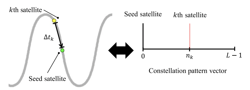
2.2 Constellation Pattern Vector
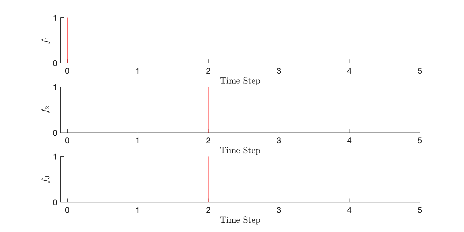
Instead of a single observer, suppose we have a set (called a constellation) of observers on the same orbit of period again discretized into L time steps. The constellation pattern vector captures the phasing of the observers in the constellation relative to a seed satellite. At time step , if the seed satellite is at position , then after time steps, the -th observer will be at position . The continuous-time time delay for the -th observer is . This is illustrated below in Figure 1.
2.3 Coverage Timeline and Coverage Requirement
The accessibility profile is a vector of binary variables describing when the target is in view of the observer as the observer travels along its orbit. The coverage timeline, denoted by , is a vector that extends the accessibility profile concept to multiple observers. At time step , describes the number of satellites with view access to the target point. Instead of a vector of binary variables, the coverage timeline is a vector of non-negative integers.
It turns out that a circular convolution between the constellation pattern vector and the accessibility profile returns the coverage timeline . The circular nature of the convolution is a direct consequence of the periodicity of the observers’ orbit. As such, can be computed from and :
Alternatively, the circular convolution can be conveniently expressed as a matrix multiplication between an circulant matrix, , and the constellation pattern vector, . Here, the -th column of is produced by circularly shifting by elements.
Expanded in matrix form and using 1-based indexing,
Often times, we are interested in satisfying a coverage requirement, , which demands a different number of observers at different time steps. The goal, then, is to place a set of observers on the orbit (i.e. find a constellation pattern ) such that the resulting coverage timeline meets or exceeds the coverage requirement . Stated mathematically,
| Find | ||||||
| such that | ||||||
| where | ||||||
2.4 Integer Linear Program Formulation
In general, there can be many constellation pattern vectors that satisfy the coverage requirement. However, it is often beneficial to minimize the total number of observers in the constellation while still satisfying the coverage requirement, since fewer observers reduce launch and maintenance costs.
The problem above of finding a constellation pattern is now a problem of finding the optimal constellation pattern that minimizes the number of observers in the constellation. The following integer linear program presents this mathematically.
| subject to | |||||
The objective is to minimize the total number of satellites, hence the objective , which sums all the entries in .
2.5 Extension to Multiple Orbits & Target Points
The above formulation is linear, and thus allows extensions to multiple target points and multiple constellations.
2.5.1 Multiple Target Points
Suppose we have a set of target points and we seek to find an optimal constellation of observers on a single orbit to monitor these target points according to a set of coverage requirements . Each target point in will have its own accessibility profile, and thus its own circulant matrix. Denote the circulant matrix for each target point by , where indexes the elements in . Then we have
| subject to | |||||
The linear constraint can be condensed into a single matrix equation by vertically concatenating the circulant matrices and coverage requirements
| subject to | |||||
2.5.2 Multiple Orbits
Suppose we have a set of orbits and we seek to an optimal constellation of observers on each orbit to monitor a single target point. Each orbit in will have its own accessibility profile, and thus its own circulant matrix. Denote the circulant matrix for each orbit by where indexes the elements in . Furthermore, each orbit will have its own constellation pattern vector, . Then we have
| subject to | |||||
The linear constraint can be condensed into a single matrix equation by horizontally concatenating the circulant matrices and vertically concatenating the constellation pattern vectors .
| subject to | |||||
We can combine the linearities above to provide a single comprehensive integer linear program. Let be the augmented constellation pattern vector obtained by vertically concatenating the constellation pattern vectors , where indexes the elements in . Let be the augmented coverage requirement obtained by vertically concatenating the coverage requirements for each target point, where indexes the elements in . Let be the augmented circulant matrix obtained by vertically concatenating the circulant matrices for each target point and horizontally concatenating the circulant matrices for each orbit. For clarity, , , and are shown in matrix form,
Thus, our full integer linear program is written as
| subject to | |||||
3 Circular Restricted 3 Body Problem
To leverage this formulation in cislunar space, a gravitational model of the region is needed. The circular restricted three body problem (CR3BP) offers an accurate model for the dynamics of a small satellite as it moves under the influence of two much larger bodies (in our case, the Earth and Moon). The equations are given by,
where U is an effective potential of the rotating system, given by
Here, is the mass ratio of the primaries and and are the distances of the object to each primary.
This formulation of the CR3BP uses normalized mass, distance, and time units which are aggregated in Table 1 below. It is important to note that the CR3BP admits periodic orbits as solutions, which is convenient for the integer linear program developed. Furthermore, the CR3BP admits 5 stationary points, called Lagrange points, where the acceleration and velocity of a satellite is zero. They are commonly referrred to as L1 through L5.
For certain accessibility measures such as the apparent magnitude of the object, the position of the sun is required in addition to that of the observer and target. In the rotating frame of the CR3BP, the sun’s motion is clockwise with period equal to the synodic period of the Earth-Moon system. A simplified model of the sun’s motion is a coplanar clockwise circular orbit of radius 1 AU around the Earth-Moon barycenter. Note that the sun is only used as an illumination source in this model. We do not consider the sun’s gravitational perturbation on the system. Parameters for the dynamics of this system are gathered in Table 1 in the appendix.
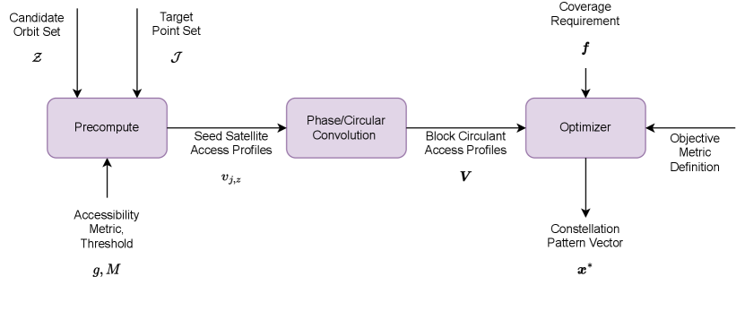
4 Utilizing the Formulation in Cislunar Space
A flow graph of the proposed formulation is shown in Figure 2 below. The first stage consists of precomputation, where we determine the accessibility for each (target point, observer location) pair in the entire constellation for the simulation period. Second, we construct the augmented circulant matrix by phasing the accessibility measures. This primarily consists of a simple circular shift operation. Lastly, we provide the necessary variables to an optimizer in the form of an integer linear program. The algorithm is outlined in pseudocode in the appendix. All orbits are discretized such that successive position states are 0.015 TU 93 minutes apart.
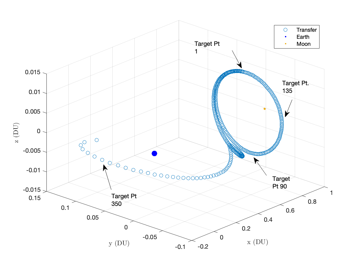
4.1 Target Point Set
As traffic between the Earth and the Moon is anticipated to increase, an attractive choice is a transfer orbit from L1 to geosynchronous Earth orbit (GEO). Figure 3 illustrates this transfer. It consists of a manifold insertion from L1 followed by a high impulse manuever into a connecting orbit to GEO. The transfer takes 23.12 days. The discretized position history (i.e. the blue circles in Figure 3) are target points comprising the set . Note that although we define as a set of points, it is actually a sequence. Target point 1 is followed by target point 2 and so on, tracking the position of a hypothetical target on this path from L1 to GEO.
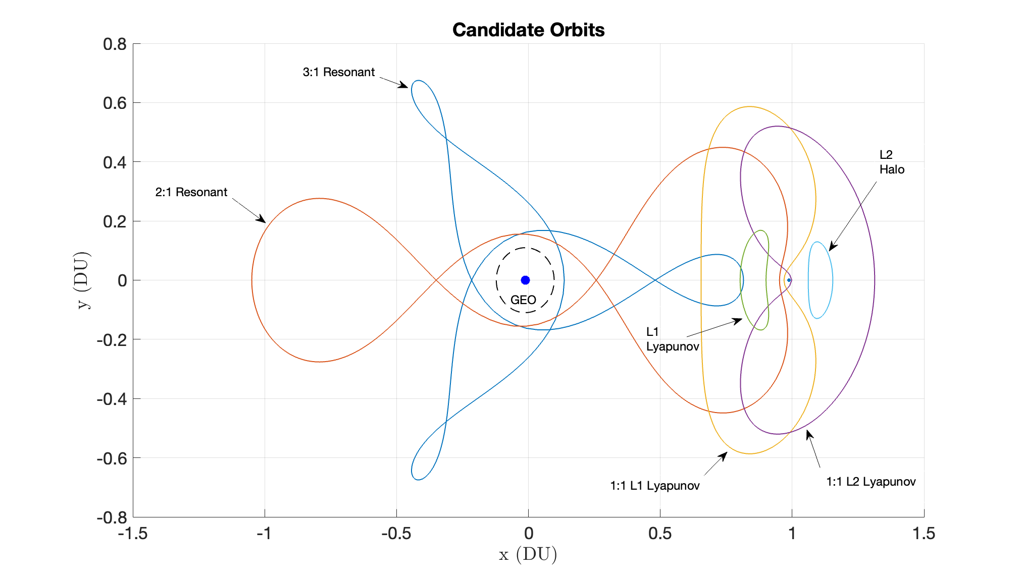
4.2 Observer Orbit Set
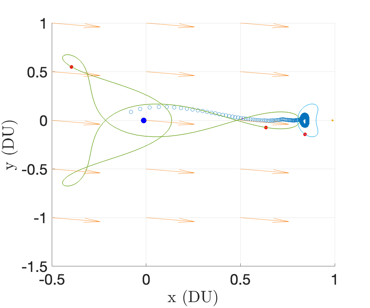
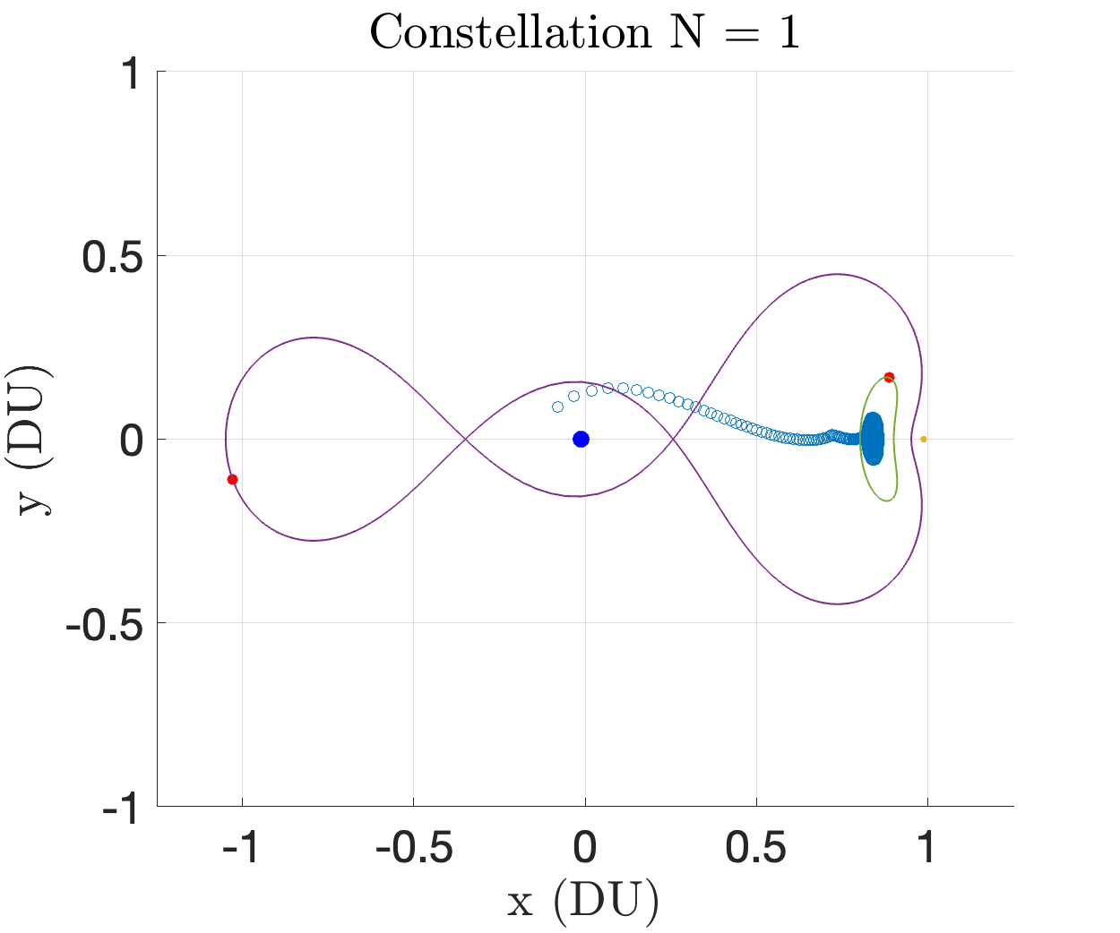
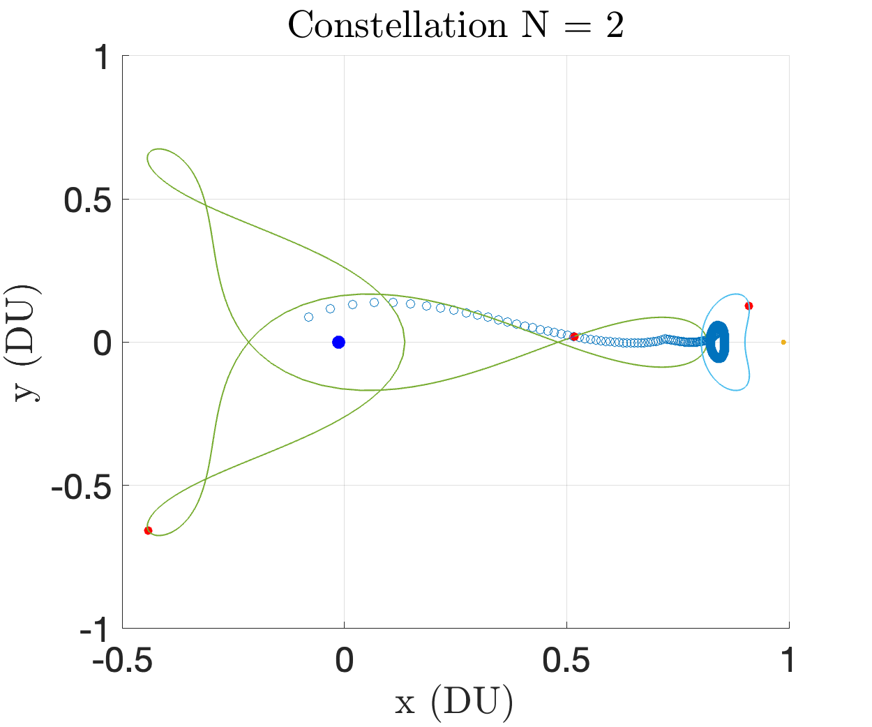
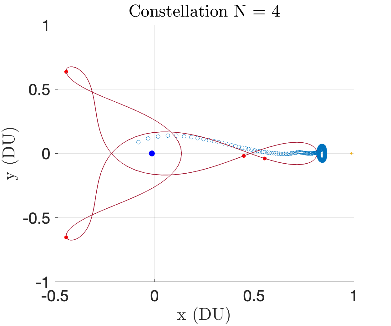
There are a variety of periodic orbits in the CR3BP. Of these, the most attractive options offer close approaches to L1 and GEO while moving through the majority of cislunar space. Furthermore, as per an AFRL objective to monitor a 30 degree cone emanating from the Earth, orbits in this region are also attractive. We choose a set of 6 orbits inspired by Gupta et al.[12], which are plotted in Figure 4 below. The initial conditions are shown in Table 3 in the appendix. All orbits were generated via a single-shooting differential correction algorithm with initial guesses sampled from data provided by NASA JPL[15] and Broucke. [16]. All orbits have period = 6.45 TU 28.008 days. It should be noted that the L1 Lyapunov and L2 Halo have a fundamental period of = 3.225 TU which means they are also -periodic. The circular restricted problem does not admit many orbits with period equal to the synodic period of the Earth-Moon system (approximately 29.05 days). As a consequence, while the orbits themselves repeat, the illumination conditions will not. As such, the results of the formalism apply on a case-by-case basis depending on the sun’s initial phase (in radians) relative to the Earth-Moon axis, denoted as . We stress that the candidate orbits are chosen to have periods as close as possible to the synodic period and are still resonant in the CR3BP sense. This ensures the difference in illumination conditions is small after TU compared to a randomly chosen constellation period. We aimed to approximately minimize this difference while preserving candidate orbit diversity. In this work we choose = 0 for optimization (Earth-Moon-Sun are collinear at simulation start). However, we investigate the robustness of the constellation to different initial phase angles later in the Results section.
4.3 Accessibility Metric and Threshold
To quantify the the observability of a target from an observer’s position, we utilize the target point’s apparent magnitude.[14],[9]Consider an observer at position , a spherical target with diameter at position , and the sun at position . Define the solar phase angle ,
It should be noted that is the familiar angle used in the dot product formula between two vectors, taking on values between 0 and . The diffuse phase angle function can be written as a function of ,
On the interval (0, ), is a strictly decreasing function. The apparent magnitude of a target is given by,
Where is the distance between the oberver and target, and are the specular and diffuse reflection coefficients of said target, respectively. Values can be found in Table 2 in the appendix. It should be noted that the solar phase angle is distinct from the initial phase angle described in the Observer Orbits section above. descibes the initial orientation of the Sun relative to the Earth-Moon axis. describes the orientation of an observer, a target point, and the Sun. The value of increases with , meaning solar phase angles closer to result in an unfavorably dim target. Every unit increase in apparent magnitude corresponds to a 2.5 times dimmer target. In addition to this, we consider the possibility that the Earth and Moon may occlude the target. If this is the case, the accessibility measure is set to , indicating an invisible target point. In practice, the measure will be set to the largest floating point number (often denoted REALMAX) available on the machine. We choose a threshold value of as our access measure cutoff. Together, and define our accessibility metric and threshold, respectively.
4.4 Coverage Requirement
We seek a set of coverage requirements, one for each target point in the set . As our object of interest travels along the transfer, it travels through each target point in order. Thus, the coverage requirement for target point should be that of target point , but shifted (in fact, circularly shifted due to the periodicity of observer orbits) forward by one index. Mathematically,
| (1) |
Where symbolizes 0-based indexing into the coverage requirement array . This recursive relation is convenient because we are only required to define the coverage requirement , with subsequent defined by Eqn. 1. An example set is illustrated below in Figure 5.
5 Results
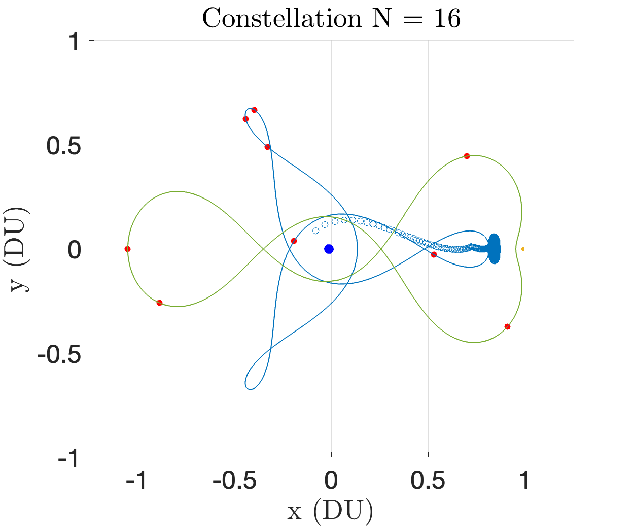
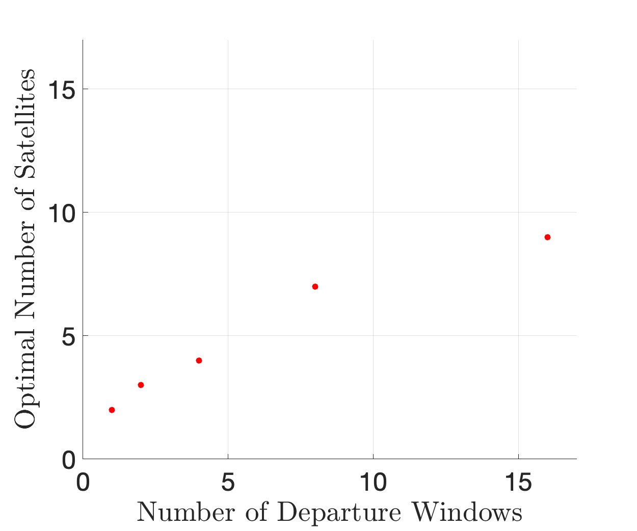
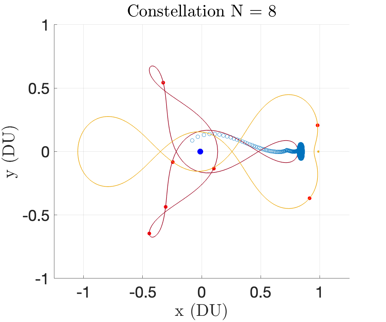
In the above image, there are two departure windows (shown as two impulses) in each coverage requirement. We choose to investigate how this number of departure windows affects the satellite constellation size. The number of requested departure windows reflects the amount of uncertainty in launch time. With more departure windows, the constellation is optimized for robustness against target departure delays. However, this will come at the cost of increasing constellation size. We specifically investigate , where the departure windows are uniformly separated amongst the time steps. The powers of two ensure that the indices where for departure windows are a subset of the indices where for departure windows, all while keeping the windows uniformly distributed in the interval . Figure 7 illustrates the result of the optimizer for departure windows. The constellation consists of 9 satellites distributed on 3:1 and 2:1 resonant orbits. These orbits were likely chosen by the optimizer because of their close approaches to the moon, where a significant portion of the spatio-temporal coverage requirement is located. Figure 14 in the appendix illustrates the results of the optimizer for every element . Figure 7 illustrates the optimal number of satellites versus the requested number of departure windows. The constellation size grows with the coverage demand. This is intuitive, since coverage potential grows with the number of observers in the constellation. We see linear growth does not hold as the coverage requirement grows. At some finite constellation size, it is expected that coverage ability saturates. Significantly stronger compute is necessary to analyze 16 departure windows . A continuous coverage requirement, i.e. , would require parallel computation for reasonable evaluation time.
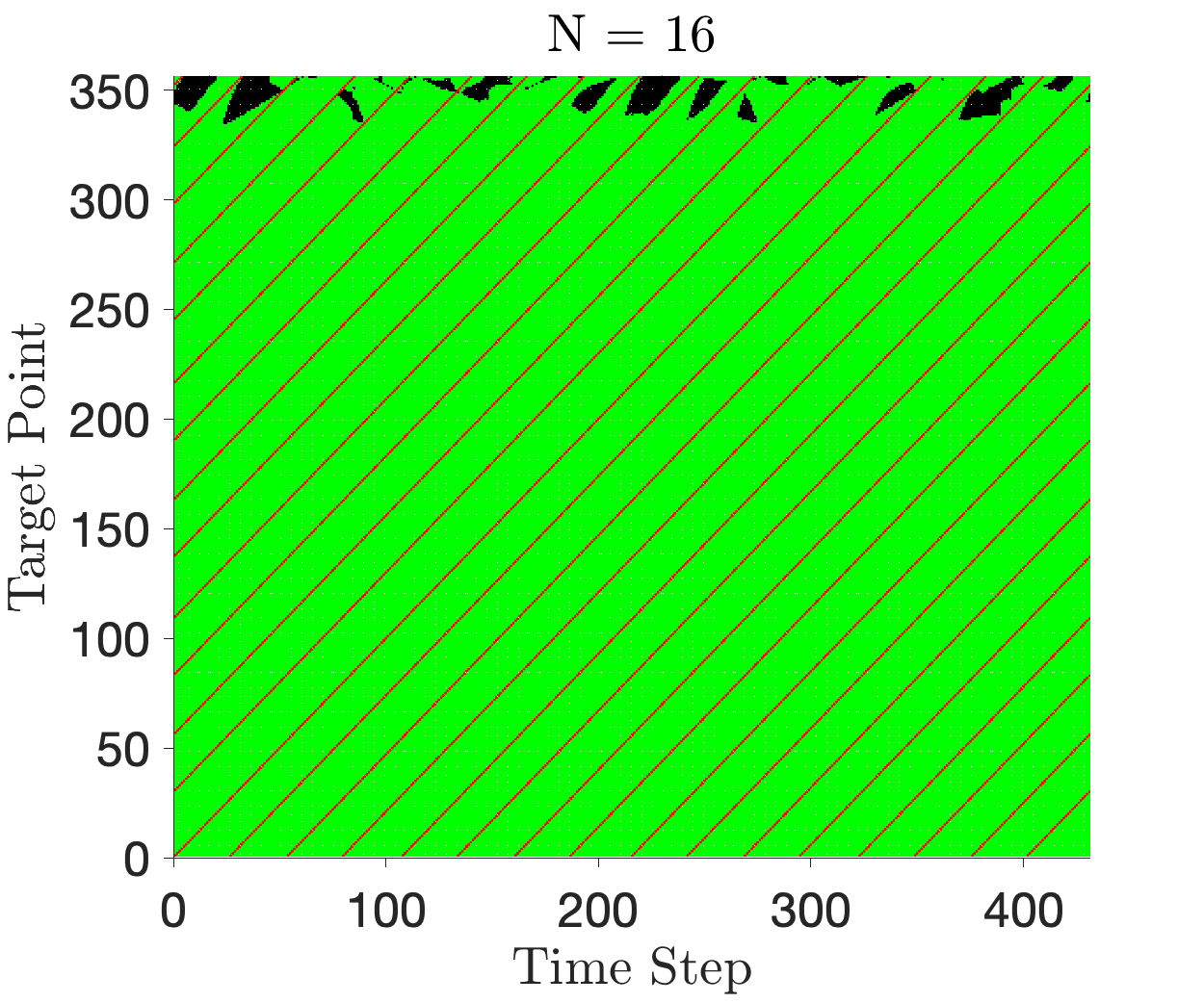
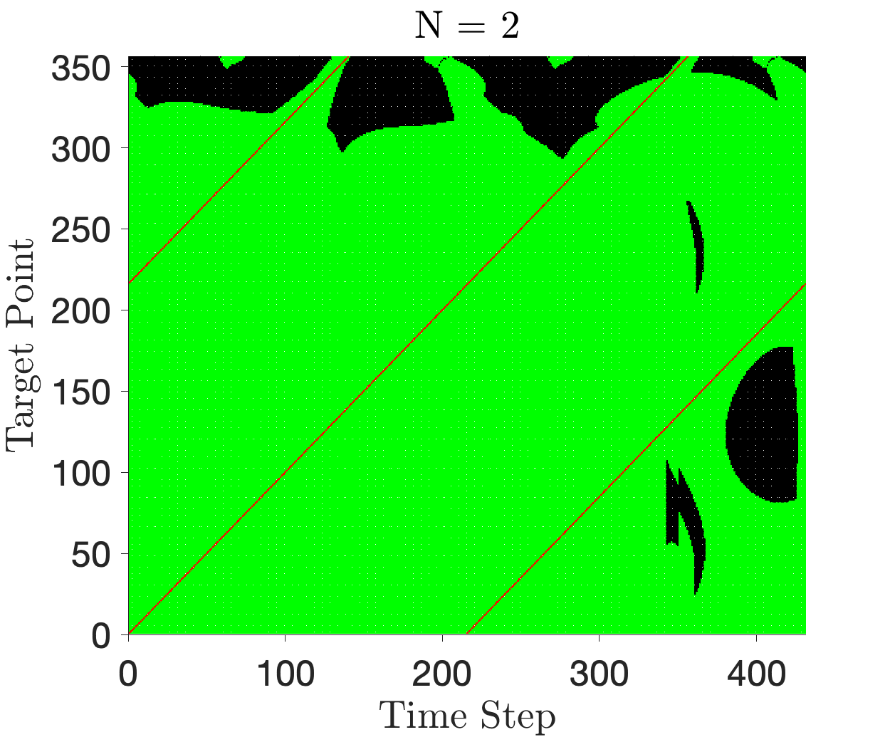
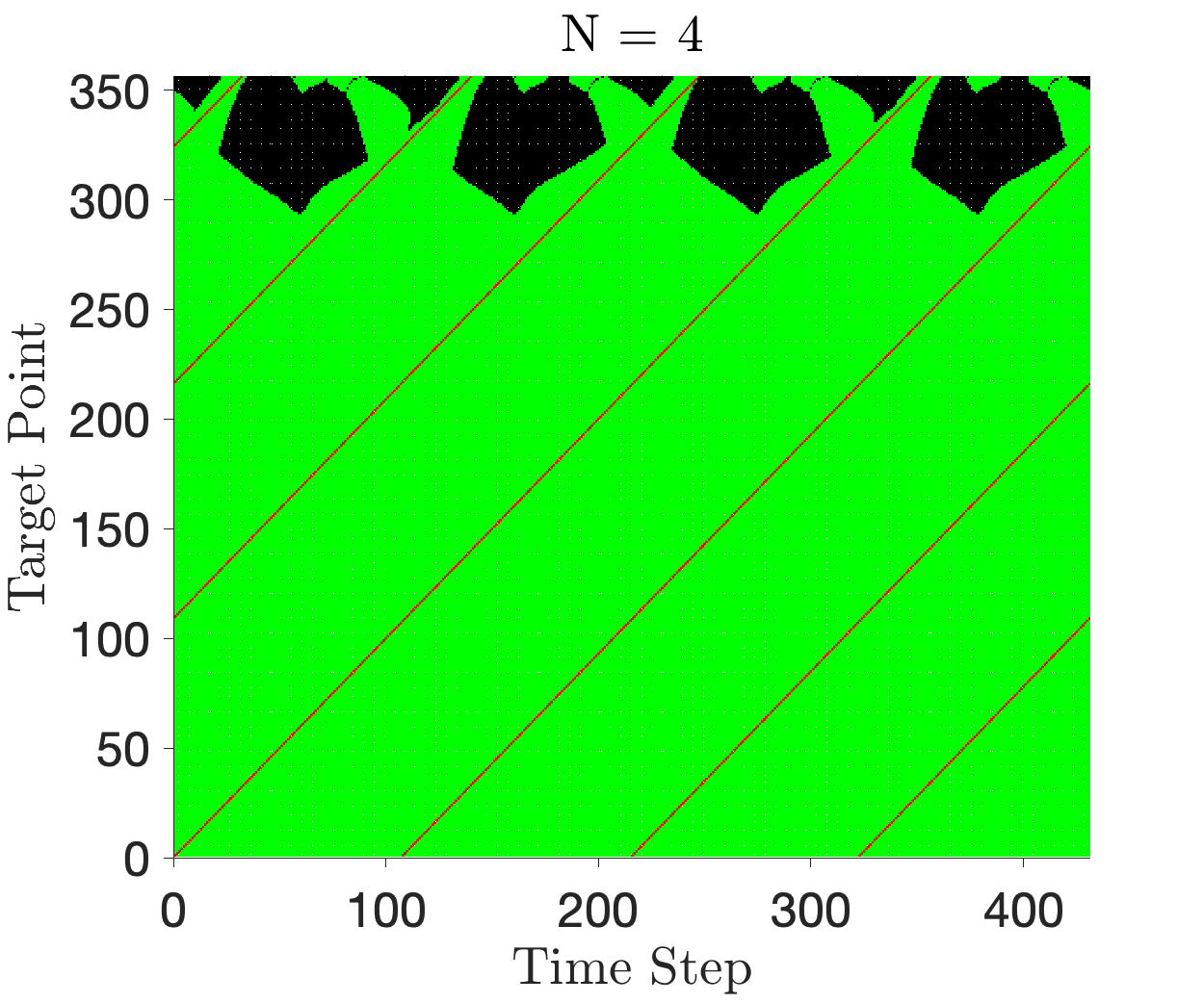
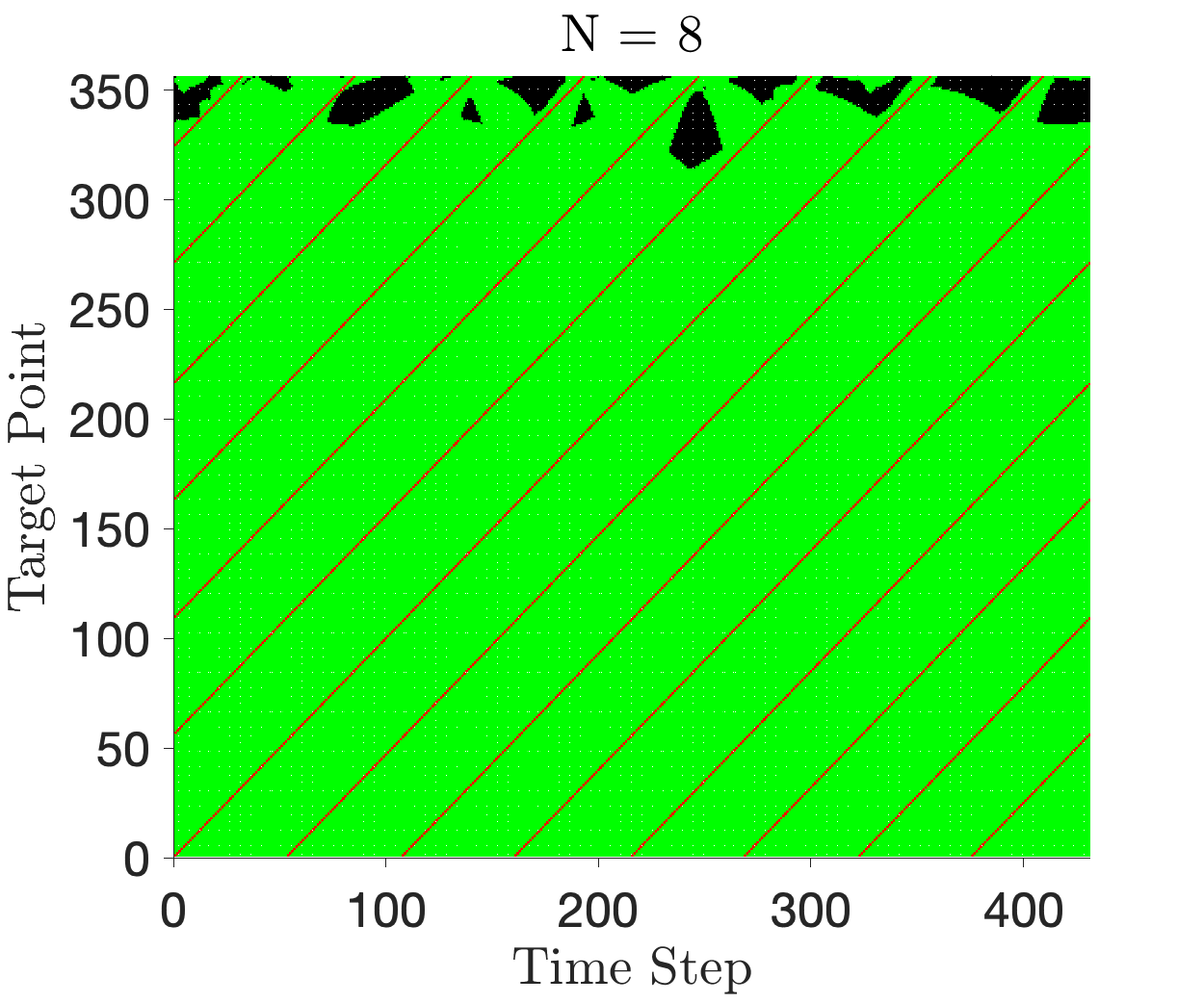
5.1 Robustness to Delays
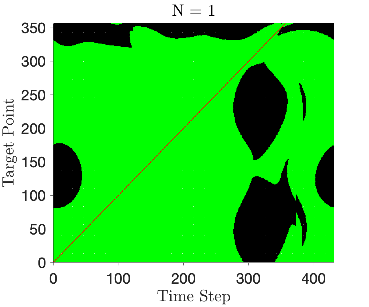
The constellation shows impressive robustness to delays in departure. Figures 9 and 9 show binary indicator maps for constellations optimized for and departure windows. Figure 15 in the appendix shows the maps for each requested departure windows. Areas shaded in green indicate a pair (Time Step, Target Point) which is observable by at least one satellite in the constellation. Areas shaded in black are not observable. The red lines (shown as diagonal streaks across Figures 9 and 9) illustrate the spatio-temporal coverage requirement sent to the optimizer. These regions are always covered, as required by the formulation. We see that the majority of the optimizer’s work attempts to cover the target points closer to GEO (target point No. 300 and onwards). As seen in Figure 3, these points are spaced further apart (the target is moving quickly in this region), naturally making it more difficult to observe. With increasing , we make progress in closing the gap, with most of the binary map displaying green for .
5.2 Robustness to Initial Sun Phase Angle,
We acknowledged earlier that because our candidate orbits are not resonant with the Earth-Moon synodic period, after one simulation period, the illumination conditions will differ slightly at the start of the second epoch ( TU). The orbits repeat but now with a slightly different initial sun phase angle, . As discussed above, we chose an initial sun phase angle of 0 rad, meaning that at the start of the simulation, the Sun is on the positive x-axis at distance 1 AU. The constellations are optimized for this phase angle, but they show impressive robustness against various initial sun phase angles. We investigated numerous between 0 and 2, given a constellation already optimized for departure windows (see Figure 15 in the appendix for an illustration of the constellation). Figure 11 shows that despite changes in , the constellation still satisfies a majority of the coverage requirement. As such, the constellation’s effectiveness extends beyond just one simulation period. For example, if mission requirements mandate a 70 coverage requirement satisfaction, then our constellation meets the mandate.
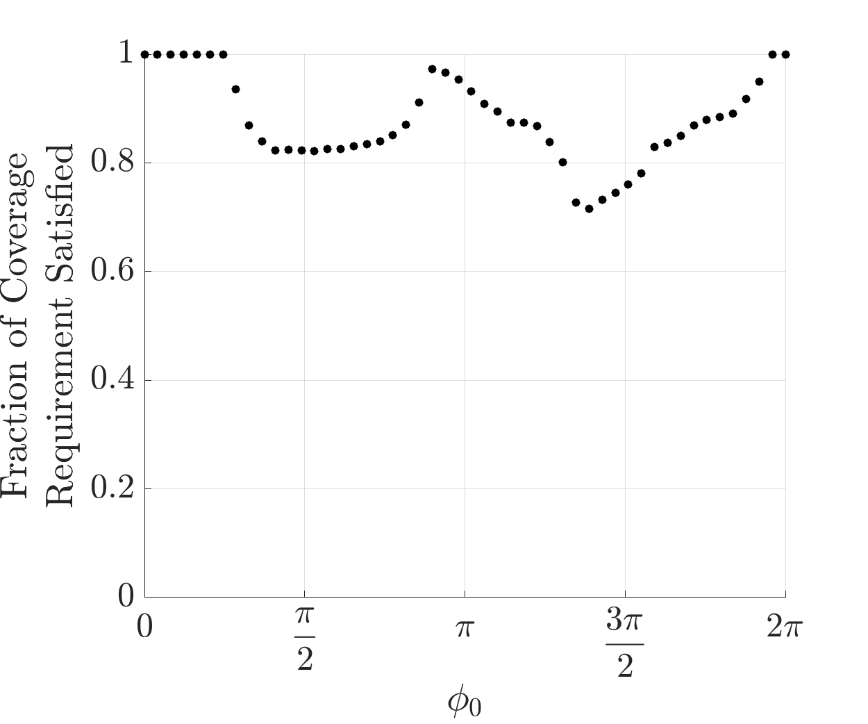
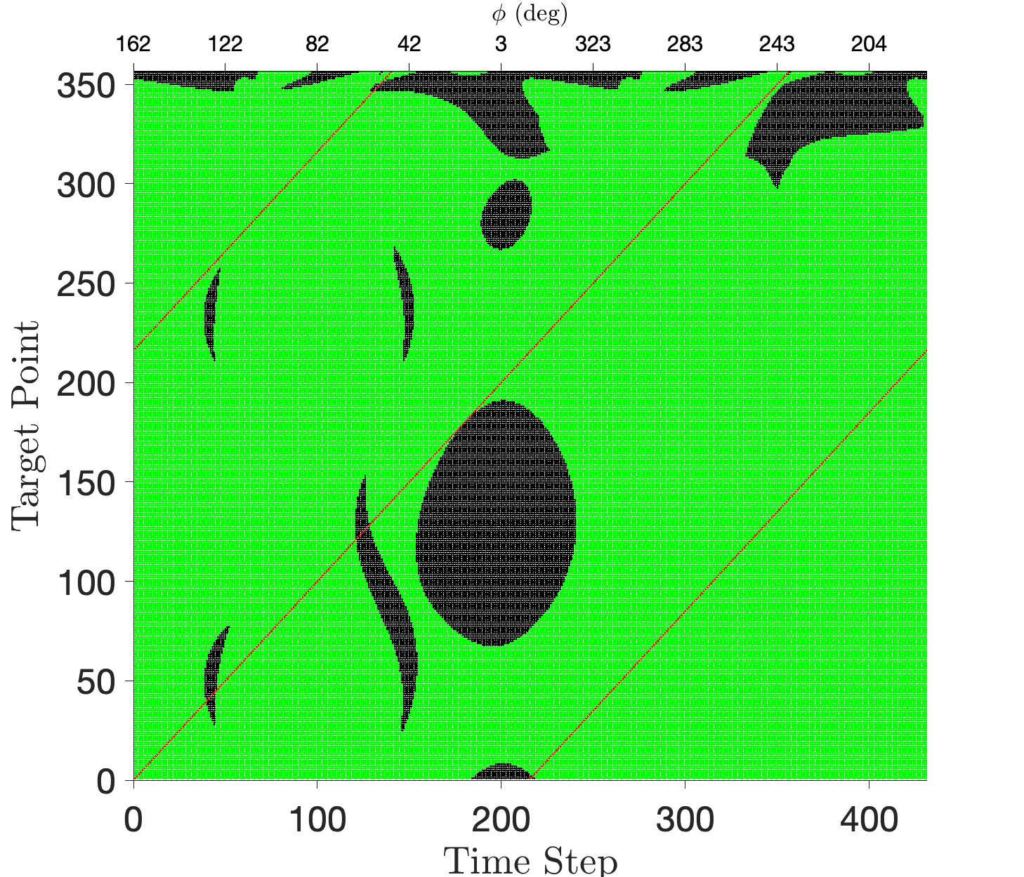
Furthermore, Figure 11 shows that there exist several values of still satisfying 90 of the coverage requirement. Figure 11 shows the coverage map for one such angle, . Not only is 97 of the coverage requirement satisfied, the impressive ratio of green to black shows that robustness to delay is still present.
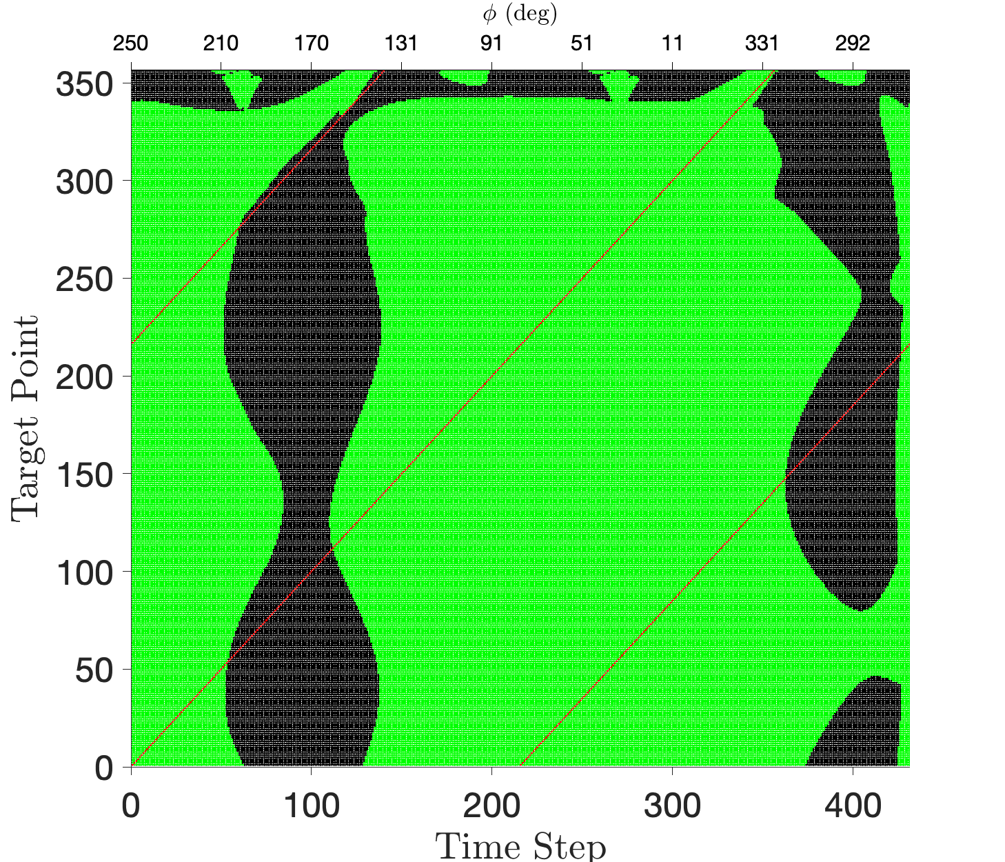
Of all the investigated in the range [0, 2], was the worst performing constellation. However, it still satisfied 71.48 of the coverage requirement. Figure 13 shows the coverage map for this choice of , illustrating that despite only satisfying 71.48 of the coverage requirement, the constellation still boasts impressive robustness to delays (shown via the ratio of green to black). There is a band of invisibility (appearing as an hourglass figure in black) in the approximate time step range 70 to 130. This is due to unfavorable solar phase angles that are incurred in this region. Figure 13 shows the position of the observers as well as the direction of the Sun’s rays at time step 100. We see that the positions of the Sun, target points, and observer on the Lyapunov orbit result in solar phase angle . In this scenario the Sun’s rays are too direct, resulting a poorly illuminated target, making it difficult for optical sensors to monitor.
6 Conclusions and Future Work
In this work we show the extension of the formulation provided by Lee et al. [13] to the cislunar regime. We show that the extension is viable in this regime due to periodic orbits present in the CR3BP. Monitoring specific transfers (such as L1 to GEO presented in this work) is possible with small constellation sizes. With more satellites, we get increasing coverage and thus, robustness to delays. This formulation can be used with any set of target points, not a trajectory specifically. This method is also fast, as illustrated by its implementation on personal computers. Significant compute is not required until the coverage requirement becomes close to continuous.
Rerunning the simulation with higher fidelity models is left to future work. Instead of the Sun on a coplanar orbit, we may incline it by to reflect the Earth-Moon system’s tilt with respect to the ecliptic. Furthermore, the Sun’s gravitational perturbation can be incorporated to determine its effect on the stability and periodicity of candidate orbits in the CR3BP. Lastly, the objective of optimization can incorporate more complex costs. We can penalize constellations that place satellites on separate orbits and include a weighting term to reflect the degree of its importance.
7 Acknowledgement
The authors gratefully acknowledge support for this research from the Air Force Office of Scientific Research (AFOSR), as part of the Space University Research Initiative (SURI), grant FA9550-22-1-0092 (grant principal investigator: J. Crassidisfrom University at Buffalo, The State University of New York).
References
- [1] D. C. Folta, T. A. Pavlak, A. F. Haapala, and K. C. Howell, “Preliminary design considerations for access and operations in Earth-Moon L1/L2 orbits,” AAS/AIAA Spaceflight Mechanics Meeting, No. GSFC-500-13-D-0037, 2013.
- [2] A. Haapala, M. Vaquero, T. Pavlak, K. C. Howell, and D. C. Folta, “Trajectory selection strategy for tours in the earth-moon system,” AAS/AIAA Astrodynamics Specialist Conference, Hilton Head, South Carolina, 2013.
- [3] P. M. Cunio, M. J. Bever, and B. R. Flewelling, “Payload and Constellation Design for a Solar Exclusion-Avoiding Cislunar SSA Fleet,” Advanced Maui Optical and Space Surveillance Technologies Conference (AMOS), 2020.
- [4] M. R. Thompson, N. P. Ré, C. Meek, and B. Cheetham, “Cislunar Orbit Determination and Tracking via Simulated Space-Based Measurements,” Advanced Maui Optical and Space Surveillance Technologies Conference, Maui, HI, 2021.
- [5] A. P. Wilmer, R. A. Bettinger, and B. D. Little, “Cislunar Periodic Orbits for Earth–Moon L1 and L2 Lagrange Point Surveillance,” Journal of Spacecraft and Rockets, Vol. 59, No. 6, 2022, pp. 1809–1820, 10.2514/1.A35337.
- [6] J. A. Dahlke, A. P. Wilmer, and R. A. Bettinger, “Preliminary comparative assessment of l2 and l3 surveillance using select cislunar periodic orbits,” AAS/AIAA Astrodynamics Specialist Conference, 2022, pp. 1–19.
- [7] E. M. Zimovan, K. C. Howell, and D. C. Davis, “Near rectilinear halo orbits and their application in cis-lunar space,” 3rd IAA Conference on Dynamics and Control of Space Systems, Moscow, Russia, Vol. 20, 2017, p. 40.
- [8] M. Klonowski, M. Holzinger, and N. Owens Fahrner, “Optimal Cislunar Architecture Design Using Monte Carlo Tree Search Methods,” 11 2022.
- [9] J. K. Vendl and M. J. Holzinger, “Cislunar periodic orbit analysis for persistent space object detection capability,” Journal of Spacecraft and Rockets, Vol. 58, No. 4, 2021, pp. 1174–1185.
- [10] L. Visonneau, Y. Shimane, and K. Ho, “Optimizing Multi-Spacecraft Cislunar Space Domain Awareness Systems via Hidden-Genes Genetic Algorithm,” The Journal of the Astronautical Sciences, Vol. 70, No. 22, 2023.
- [11] C. Frueh, K. Howell, K. DeMars, S. Bhadauria, and M. Gupta, “Cislunar space traffic management: Surveillance through earth-moon resonance orbits,” 8th European Conference on Space Debris, 2021.
- [12] M. Gupta, K. C. Howell, and C. Frueh, “CONSTELLATION DESIGN TO SUPPORT CISLUNAR SURVEILLANCE LEVERAGING SIDEREAL RESONANT ORBITS,”
- [13] H. W. Lee, S. Shimizu, S. Yoshikawa, and K. Ho, “Satellite Constellation Pattern Optimization for Complex Regional Coverage,” Journal of Spacecraft and Rockets, Vol. 57, Nov. 2020, pp. 1309–1327, 10.2514/1.A34657.
- [14] W. E. Krag, “Visible magnitude of typical satellites in synchronous orbits,” Sept. 1974.
- [15] M. Vaquero and J. Senent, “Poincare: A Multi-Body, Multi-System Trajectory Design Tool,” 2018, 2014/48975.
- [16] R. A. Broucke, Periodic orbits in the restricted three-body problem with earth-moon masses. 1968.
- [17] C. Rackauckas and Q. Nie, “DifferentialEquations.jl–a performant and feature-rich ecosystem for solving differential equations in Julia,” Journal of Open Research Software, Vol. 5, No. 1, 2017.
Appendix A Appendix
A.1 CR3BP System Parameters and Candidate Orbit Initial Conditions
System parameters for the Earth-Moon CR3BP with the Sun as illumination source are presented in Table 1. Initial conditions for candidate orbits are shown below in Table 3. Orbits were generated via a single shooting differential corrections algorithm written in Julia. We use the Vern7 ODE propagator (available in the Julia DifferentialEquations[17] module) in this algorithm.
| Table 1: CR3BP Parameters | |
|---|---|
| Parameter | Value |
| Mass parameter, | 1.215058560962404e-02 |
| Length scale, DU (km) | 384400.0 |
| Time scale, TU (s) | 3.751902619517228e+05 |
| Relative distance of Sun (DU) | 389.17794 |
| Angular velocity of Sun (rad/TU) | -0.9253018261815922 |
| Earth Radius, (km) | 6371 |
| Moon Radius, (km) | 1737.4 |
| Table 2: Illumination Parameters | |
|---|---|
| Parameter | Value |
| Sun apparent magnitude, | -26.74 |
| Target specular reflection coef., | 0.0 |
| Target diffuse reflection coef., | 0.2 |
| Target Diameter, (km) | 0.001 |
| Table 3: Candidate Orbit Initial Conditions | |||
| 3:1 Resonant | 2:1 Resonant | 1:1 L1 Lyapunov | |
| 0.13603399956670137 | 0.9519486347314083 | 0.65457084231188 | |
| 0 | 0 | 0 | |
| 0 | 0 | 0 | |
| 1.9130717669166003e-12 | 0 | 3.887957091335523e-13 | |
| 3.202418276067991 | -0.952445273435512 | 0.7413347560791179 | |
| 0 | 0 | 0 | |
| T | 6.45 | 6.45 | 6.45 |
| 1:1 L2 Lyapunov | L1 Lyapunov | L2 Halo | |
| 0.9982702689023665 | 0.8027692908754149 | 1.1540242813087864 | |
| 0 | 0 | 0 | |
| 0 | 0 | -0.1384196144071876 | |
| -2.5322340091977996e-14 | -1.1309830924549648e-14 | 4.06530060663289e-15 | |
| 1.5325475708886613 | 0.33765564334938736 | -0.21493019200956867 | |
| 0 | 0 | 8.48098638414804e-15 | |
| T | 6.45 | 3.225 | 3.225 |
A.2 Optimizing the Constellation Pattern Vector
Algorithm 1 presents pseudocode for the formulation. In this work, we utilize Gurobi MATLAB for computation. Computation is done with an M1 Pro CPU using 8 high-performance cores. Algorithm run time is 300 seconds for each .
A.3 Extended Results
Figures 14 and 15 show the constellations and indicator maps of all the optimization runs for each .
 |
 |
 |
 |
|
|
|
 |
 |
 |
|