Classical Analog of Quantum Models in Synthetic Dimensions
Abstract
We introduce a classical analog of quantum matter in ultracold molecule- or Rydberg atom-synthetic dimensions, by extending the Potts model to include interactions between atoms adjacent in both real and synthetic space and studying its finite temperature properties. For intermediate values of , the resulting phases and phase diagrams are similar to those of the clock and Villain models, in which three phases emerge. There exists a sheet phase analogous to that found in quantum synthetic dimension models between the high temperature disordered phase and the low temperature ferromagnetic phase. We also employ machine learning to uncover non-trivial features of the phase diagram using the learning by confusion approach. The key result there is that the method is able to discern several successive phase transitions.
I Introduction
Recently experiments on synthetic dimensions – where transitions between non-spatial degrees of freedom can be regarded as motion in an additional lattice direction – have explored physics difficult to realize in real space, such as topological band structures and phases Lin et al. (2016); Dutt et al. (2019); Kanungo et al. (2021), gauge potentialsYuan et al. (2018), and spatially-resolved non-linear dynamics An et al. (2021). Introduced in Ref. Boada et al. (2012), synthetic dimensions were later explored in several platforms, including with synthetic sites formed from momentum states or states of light Ozawa and Price (2019).
We are motivated by synthetic dimensions formed by periodic arrays of ultracold polar molecules or Rydberg atoms in optical lattices or microtrap arrays, specifically a two-dimensional (real space) square lattice. The rotational states of molecules or electronic states of the Rydberg atoms provide the sites of a synthetic third dimension, and microwaves induce tunneling matrix elements between the synthetic lattice sites. These systems are described by the quantum many-body Hamiltonian Sundar et al. (2018); Kanungo et al. (2021),
| (1) |
The first term describes tunneling between synthetic sites at each real-space site , induced by a resonant microwaves, while the second term describes an interaction in which atoms or molecules on nearest-neighbor real-space and synthetic sites exchange their synthetic positions. indicates a sum over nearest real-space neighbors. Longer-ranged real-space interactions are also present in experiments, but the nearest-neighbor truncation is likely to describe many of the qualitative features of the phase diagram.
Since each molecule occupies a unique real-space site, the relevant subspace satisfies . In general and depend on , the choice of internal states, and the microwave drives, but in the simplest cases they are independent of Sundar et al. (2018).
Some interesting physics has been predicted for these systems: whereas the hopping leads to delocalization in the synthetic direction, the interaction drives “sheet formation”: for low temperature and large , molecules on adjacent sites will share a common pair of rotational states , flattening the system in the synthetic direction, though with quantum and thermal fluctuations. So far, predicted phase diagrams have been limited to simple variational techniques Sundar et al. (2018), exact solutions in one real dimension Sundar et al. (2019), or certain sign-problem free regions and observables with Quantum Monte Carlo (QMC) methods Feng et al. (2022), which have only begun to be explored.
Equation (1) can also be viewed as a large-spin spin models, with the size of the spin set by the number of synthetic sites , albeit with interactions and symmetries that are unusual or awkward to describe in the spin language. (especially in the general case where the or have interesting dependences on n) In this way, there is a similarity to the classical Potts or clock models, where there are likewise possible choices for the variable at each site, with a single one of them ‘occupied’ in any given configuration.
However, while corresponding classical spin models would provide important guidance for the physics of the quantum model, the analogy to classical Potts or clock models has serious shortcomings. The Potts model is invariant under permutations of any of the spin components, a much larger symmetry than the translation symmetry obtained by translating by one site in the synthetic direction (assuming a large synthetic dimension or periodic boundary conditions). This potentially can cause the Potts model analog to host unrealistically large fluctuations and varieties of symmetry breaking phases. The clock model is another analog classical model, and it enjoys the correct translation symmetry for translating spin indices. However, it has couplings between all spin states, even ones that have large [] separations in the synthetic dimension, in contrast to the local nearest-synthetic-neighbor couplings in the synthetic dimension model Eq. (1). (Potts and clock models are discussed in more detail below.) Wu (1982); Ortiz et al. (2012); Li et al. (2020)
In this paper, we introduce a classical analog model capturing the salient features of synthetic dimensions that remedies these deficiencies of the Potts and clock models. We do this by extending the Potts model to include an additional nearest-synthetic-neighbor term, , to the Potts model, as described in the next section, which breaks the permutation symmetry to a translation symmetry (unlike the naïve Potts), while preserving locality in the synthetic dimension (unlike the clock model).
Although our motivation is to examine a simple version of a quantum model of synthetic dimension, as we shall discuss, our variant of the Potts model itself has a rich phenomenology, including a non-monotonic behavior of the critical temperature as a function of , and the formation of sheet states in analog to the quantum membrane states in the corresponding quantum model. It also offers an interesting context in which to extend machine learning methods for statistical mechanics. While our study could certainly be viewed simply as an interesting extension of a traditional spin model, considering it in the language of synthetic dimension provides additional context to the work, as well as potential experimental (cold molecule/Rydberg atom) connections.
We also note that, interpreted as spin models, synthetic dimensions have obvious parallels in the condensed matter context. The different angular momentum states in and electron systems can be considered as a synthetic site index, though in most real solids one-body effects like crystal field splitting break the orbital degeneracy and reveal the true “spin nature” of the model, limiting its interpretation as an additional dimension. Nevertheless, the classical model we introduce may have commonalities with the interactions in real materials, and suggests phases that may occur there.
After introducing the model and our primary computational methodology (Sec. II), we will examine the physics within a mean field theory (Sec. III) before presenting numerically exact calculations of properties with Monte Carlo, and inferences for the phase diagram (Secs IV, V, and VII). We will then turn towards a machine learning approach to analyzing the results (Sec. VI), and finally summarize our conclusions.
II Model and Monte Carlo Methodology
The Potts model Wu (1982) is a generalization of the Ising model in which the degrees of freedom on each lattice site take on possible values, with the Ising model corresponding to . The energy is when adjacent share a common value, and zero otherwise. A considerable literature exists concerning the Potts model, with many generalizations, including multi-spin interactions, dilution, external fields, etc. The physics of these is well explored, both analytically and numerically in Ref. Wu (1982). Relevant to the work presented here, the two-dimensional Potts model exhibits a first order phase transition when .
We add a term to the Potts model to describe a situation in which the energy is also decreased by if neighboring spins differ by . That is,
| (2) |
We denote by the number of spatial sites of a lattice with linear dimension . It’s reasonable to employ a Periodic Boundary Condition (PBC) in both the real dimensions as well as the synthetic dimension. In this language, the additional term corresponds to a coupling favoring molecules on neighboring sites having adjacent positions in the synthetic dimension, such as is present in the term of Eq. (1). In the results which follow we set as our energy scale.
For , Eq. 2 is the same as the Potts model with (for . Thus our model would share all Pott’s properties, including a second order transition at . This exact mapping is true only for , but is nevertheless suggestive. We do not study the small limit further here, since, in extending the interactions to include also and , for small the “range” (three) becomes close to the “lattice size” in the synthetic direction.
The clock model Ortiz et al. (2012); Li et al. (2020) is another well known description of classical phase transitions admitting a controllable discrete set of values on each site. It should be noted that, as is the standard notation, the number of Potts degrees of freedom is denoted by , with being used for the Clock model. The clock model energy is,
| (3) |
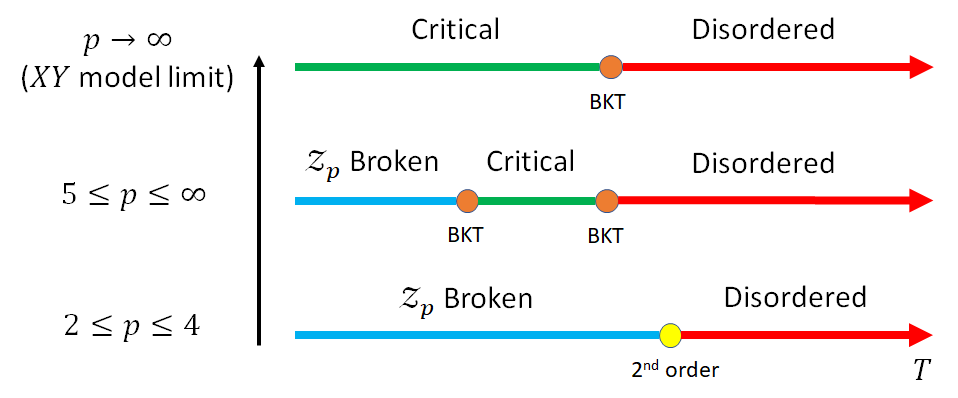
The clock model shows qualitatively different behavior at different values, as we will demonstrate happens in our model as well. Fig. 1 shows the phase diagram of the clock model. Unlike the Ising and Potts models, which have single critical points, the clock model, for exhibits two distinct transition temperatures, between which there is a Berezinskii-Kosterlitz-Thouless (BKT) phase. The higher-temperature transition occurs at a critical temperature , while the lower transition has , vanishing in the XY limit . These two distinct transitions occur because the breaking of the full continuous symmetry of the XY model is irrelevant for temperatures above when José et al. (1977); Cardy (1980). As we will show in the sections below, Eq. 2 exhibits similarity to the clock model in the sense of exhibiting three phases, with an intermediate ‘sheet phase’ separating the high temperature disordered and low temperature breaking phases.
To explore the statistical mechanics of Eq. 2 quantitatively, we will primarily use the simple classical single site update Metropolis Monte Carlo method. We measure observables including the internal energy , the specific heat , and the average synthetic distance between neighboring real-space sites, where
| (4) |
The summation runs over all neighboring sites and , and measures the distance of site and in the ‘synthetic dimension’. The normalization is to the number of bonds on the square lattice. is defined to loosely capture a transition into a “sheet” phase between a low temperature phase where all are identical and the high temperature disordered phase. We will define this sheet phase more precisely in Section 4.
To characterize the phases further, we define
| (5) |
which measures the fractional likelihood that the synthetic distance between near neighbor sites is exactly . and are related by .
III Mean Field Theory
The mean field theory of the standard, many-state Potts model can be found, for example, in Mittag and Stephen (1974). The addition of a second energy scale for next nearest neighbors presents some new features which we now consider. For ease of computation, we assign the Potts spin at one site an accompanying spin variable (). Here, is the complex increment between spin variables. We then use the identity,
| (6) |
which allows us to convert Kronecker delta functions in the Hamiltonian to products of spin variables and . Applying this definition to Eq. 2, the energy between two sites is
| (7) |
We introduce the mean field by defining a set of order parameters, Mittag and Stephen (1974). serves as the ‘alignment’ of the mean field and can take on values of ; if is , then the field is aligned relative to (akin to an origin). As the Potts model views neighboring sites as being the same spin, off by one, or of any other value, we are free to choose our field alignment and hence set for convenience. Replacing the spin variable with order parameter leaves us with
| (8) | |||
| (9) |
where is the number of nearest neighbor sites ( for a square lattice). Taking the expectation value and setting it equal to , we arrive at the self-consistent equation
| (10) |
which at reduces to the self-consistent equation of the standard Potts mean field theory Mittag and Stephen (1974).
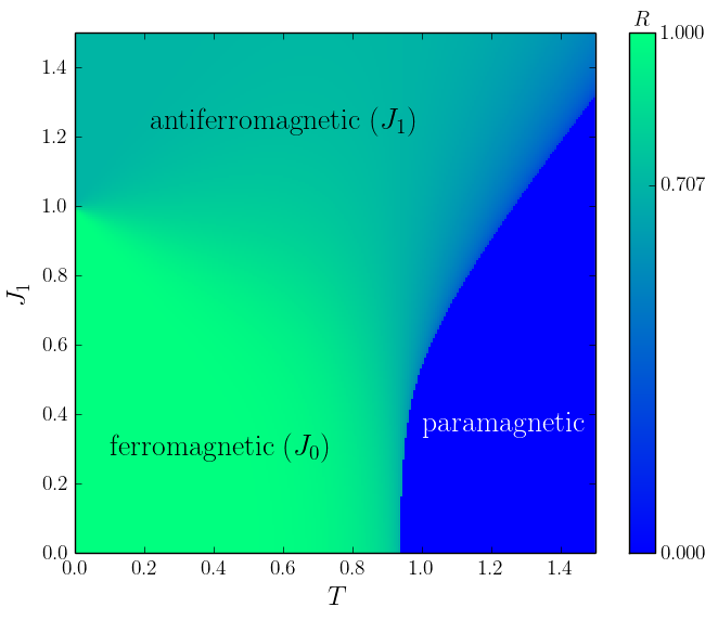
The resulting phase diagram with is given in the heat map of Fig. 2. The blue region shows the high temperature, disordered phase where the order parameter . For there is the ‘conventional’ low ferromagnetic phase of the Potts model (bright green) where Potts variables on different sites are identical. However a second ordered phase appears (cool green) for in which for . In this region, the Potts variables on adjacent sites differ by . We refer to this as an ‘antiferromagnetic’ regime since adjacent spins are forced to take distinct values. We will argue, based on the approximation-free Monte Carlo solution in the next section, in which we can take more sensitive ‘snapshots’ of the spin configuration, that an additional intermediate regime arises in which the Potts variables on adjacent sites are either identical, or differ by . In the heat map of Fig. 2, this behavior is seen in the dark blue region that emerges for , where as if the system was allowing for the coexistence of nearest- and next nearest-neighboring interactions between ferromagnetic and antiferromagnetic ordering. The critical point at is consistent with the analytic value for .
IV and for and
We turn now present results obtained with Monte Carlo.
It is known for the pure clock model that is a critical value for the appearance of a BKT phase at intermediate temperature, and that the phase diagram is qualitatively the same for any , i.e. differing only in the range of temperature over which the intermediate phase is stable, as seen in Fig. 1. Similarly, we observe a intermediate regime that differs from the ground state behavior for in our model as well. To explore the novel intermediate region, we focus our study on just two values: and . This choice also allows us to gain some insight into quantitative changes with without excessive redundancy. We will demonstrate later that instead of creating pairs of vortexes as in the clock model, a ‘sheet’ is formed in the intermediate temperature region when the interaction sufficiently strong.
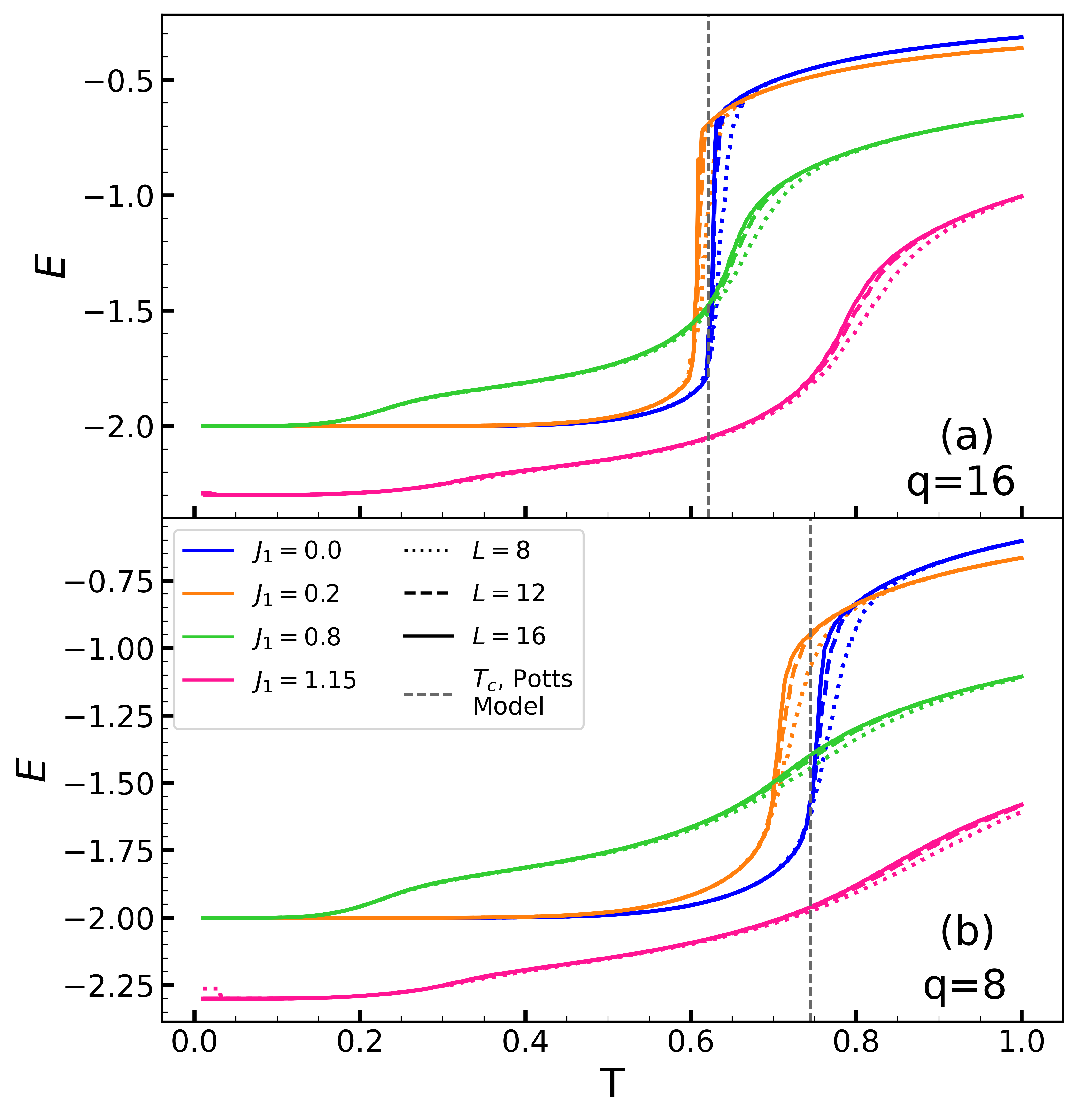
We begin by showing the energy per site for with (Fig. 3a) and (Fig. 3b). For the ground state has all the sites taking the same spin value, and an energy per site . We will call this ground state the Ferromagnetic (FM) phase. For , it is energetically favored to have adjacent sites with so that at . We call this the Antiferromagnetic (AFM) phase. In both panels, the known first order transition at of the conventional Potts model () is shown for comparison. This first order character remains evident at small , however, occurring at a (slightly) reduced . We interpret the lowering of to arise from the fact that initially competes with the tendency of to make all values of identical.
As increase further, however, begins to grow. Here our picture is that the two interactions behave in a more cooperative way, raising the critical temperature. Notably, it can be seen that when is small, predicted by mean field theory is slightly higher than that predicted by Monte Carlo data, which is to be expected, as mean field theory overestimates by neglecting fluctuations. Simultaneously, the evolution of becomes more gradual, suggesting a continuous phase transition, or even a crossover. Studies on a finer mesh of indicate the change of order of transition appears to coincide with the value of for which is minimized. As can be seen from the curve, aside from the now-continuous transition at , a second feature emerges at . This is a first indication of the existence of an intermediate regime.
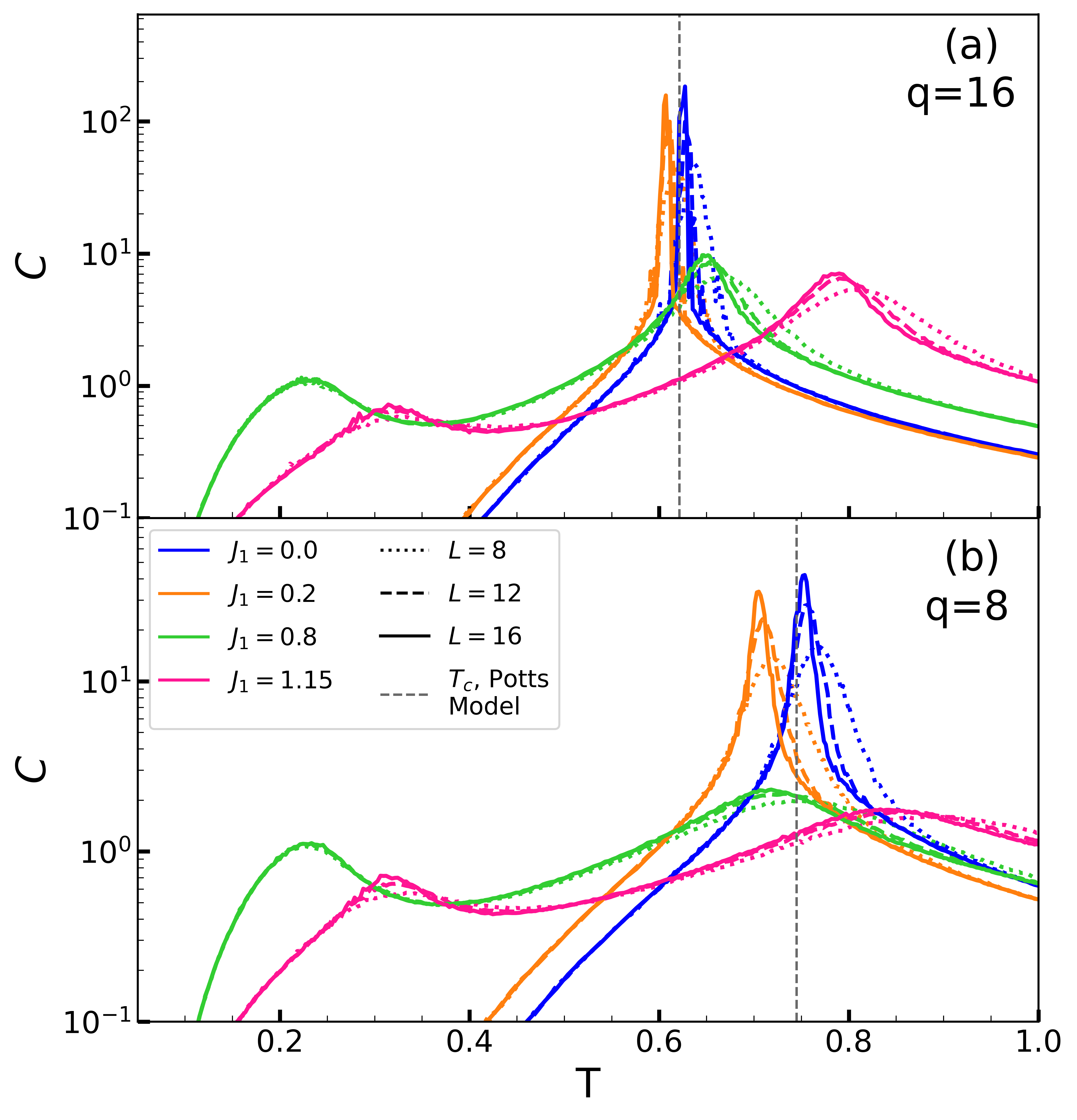
The change from first-order character is further revealed in the specific heat. Figure 4 gives for the same sequence of , again for and . For , the first-order discontinuity of in the thermodynamic limit is signalled by the very large value of the finite lattice derivative, exceeding by more than an order of magnitude the peaks at where the transition is second order. Framed more precisely, at a first order transition the specific heat on a finite lattice scales as the volume of the system, , whereas for a second order transition . Here and are the critical exponents for the specific heat and correlation length respectively. As a consequence, the specific heat peaks are much smaller in the second order region.
As noted already in the data for , Fig. 3, for an additional, lower temperature, specific heat peak emerges. This suggests the existence of an intermediate regime between the ordered phase at low temperature and the disordered phase at high temperature. We shall focus our discussion to the intermediate regime in the next section. Given the qualitative similarity of the results for and , in the next section we will restrict our analysis to the larger value of .
V Sheet Formation
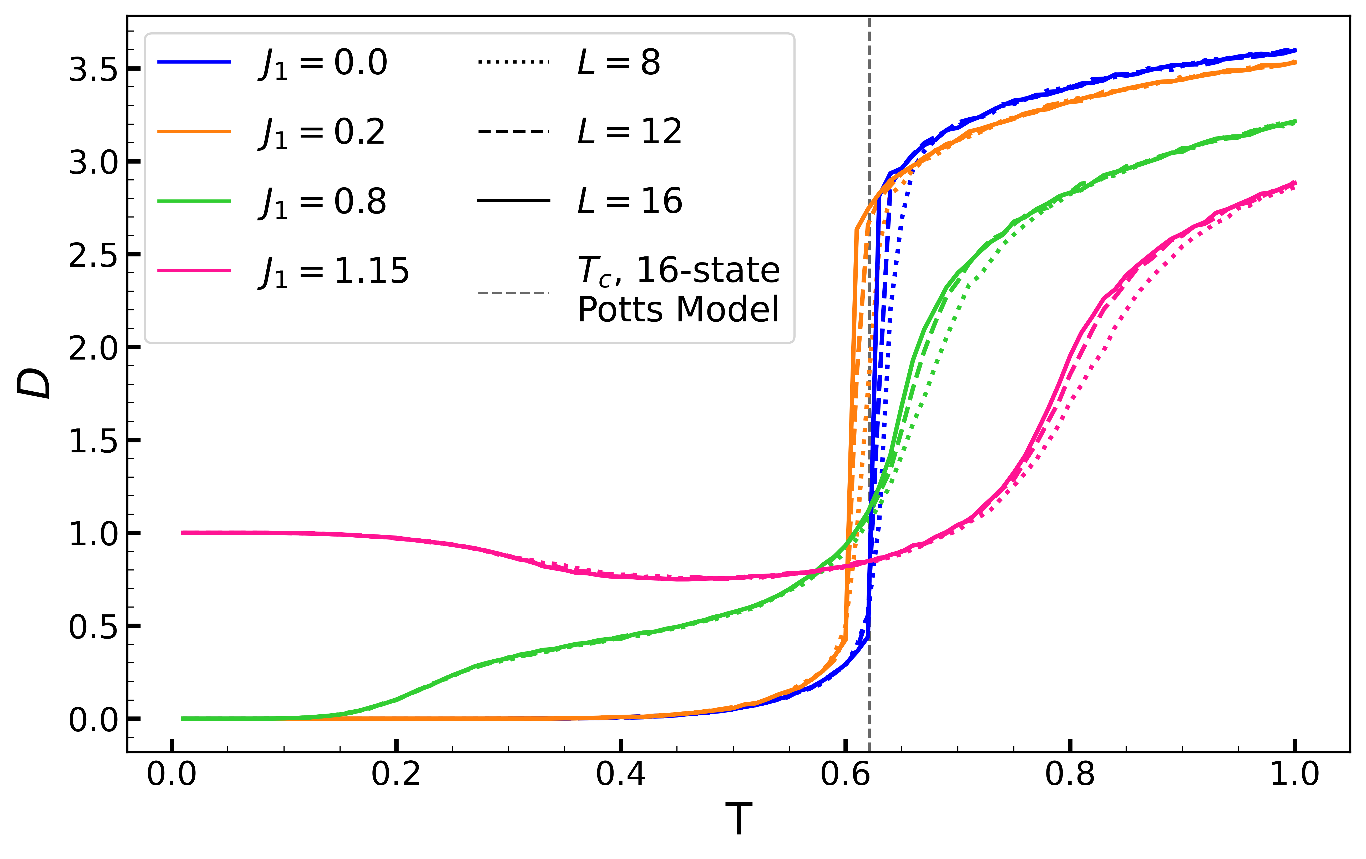
We now turn to examining the nature of the intermediate region, in which we believe a ‘sheet’ forms, analogous to that of the quantum model Feng et al. (2022). Fig. 5 shows the average distance in synthetic dimension between nearest neighbors on the lattice, as a function of , for and , that is, horizontal sweeps of the phase diagram of Fig. 2. For all values, we see asymptote at high temperature to , which indicates a disordered phase where the spins randomly (probability ) and independently occupy different synthetic position.. (Note our use of PBC in the synthetic direction imposes a maximal value .)
For and , increases from to the high temperature limit of through a direct jump, suggesting a single first order phase transition from the ordered phase to the disordered phase, like the Potts model. However, for , shows a plateau which coincides with the temperature range between the two specific heat peaks in Fig. 4. In this region, is sufficiently strong to allow neighboring spins and to take on values in addition to favored by . The precise value of depends on , which will control the relative likelihood of and . If those cases are all equally probable, for example, then . We will refer to this as the sheet phase, because spatially neighboring spins exist in a range of three adjacent values, and, as we shall see, this persists to larger separations, so that the configuration looks like a sheet in dimensions. This is to be distinguished from the Ferromagnetic phase, where all spins are identical.
For , the ground state is different. at low temperature is expected now since all the neighboring spins favor taking values that differ by one. This change of ground state can be checked in the limit of in Fig. 3, which takes on the value of as expected. With increasing , neighboring spins in the system start to take on values that are the same, thus the system enters the sheet regime, before going into the disordered phase at high temperature, as was the case with . That the intermediate region of and are of the same nature, and no transition is between them, will be corroborated below.
The existence of the intermediate sheet region can be qualitatively understood by looking at the system’s free energy. For , at very low but finite temperature, excited states become accessible. The lowest-energy excitations are the ones where one site takes a spin value that differs by one from its neighbors’. This costs an energy of . Comparing to a Potts model with , it’s evident that our model should retain its FM order for a range of finite low temperatures, since all of its excitations cost more energy than that of the Potts model’s, which is know to have a FM ground state at low temperature. However, upon increasing , a manifold of excited states that we call ’sheet state’ will proliferate. The sheet state refers to a state where all the neighboring spins take on spin values that are either the same or differ by one. Such states have extensive energy , and entropy per site . The latter can be understood by a counting similar to that of degenerate ground states for , which is outlined in the Appendix Classical Analog of Quantum Models in Synthetic Dimensions. This means sheet states will have a free energy contribution , which goes negative at . We will show in the next paragraph that the system makes a transition into a sheet-state regime at a finite temperature for for . As we continue to increase , the system will go into a disordered state as expected. We recall that it was also observed in and plots that at the same where sheet phase appears, the transition to the high temperature disordered phase becomes continuous. We argue that this is plausible as the system in the sheet regime could have different symmetry from its ground state. This also raises the question of whether the transition from the ground state to the sheet regime is a true phase transition. We will come back to this question when discussing the phase diagram.
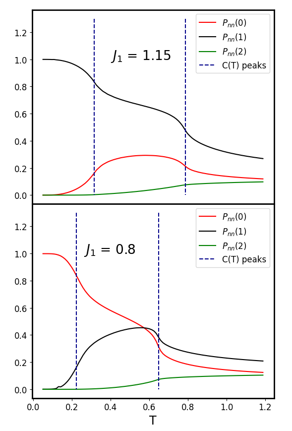
To support the existence of the sheet regime further, we measure . In the upper panel, we see while both and at low for . This tells us all the spins are taking the same value as they should in the FM phase. As we increase past the temperature of the lower heat capacity peak, starts to drop significantly, while increases. Meanwhile is still very close to . This is to say, in this region, neighboring spins are equally likely to take values that are identical and off by one, but they dislike taking values that are further separated, the defining characteristic of the sheet phase, and consistent with Fig. 5. As we increase further, all the curves go to the same limit, resembling the disordered phase where all spin values are equally likely.
Similarly, in the upper panel, the low limit of is showing a clear feature of the AFM phase. In the intermediate region between the two heat capacity peaks, the decrease of and the increase of are both significant, while is kept at a low level. This is similar to the behavior at . The difference is that here we’re coming to the sheet regime from an AFM phase instead of a FM phase. This picture will be validated by the machine learning method explained in the next section.
VI Machine Learning Approaches
Both supervised and unsupervised machine learning algorithms have been used recently to find critical points of classical and quantum models of magnetism Wang (2016); Hu et al. (2017); Carrasquilla and Melko (2017); Zhang et al. (2019); Canabarro et al. (2019); van Nieuwenburg et al. (2017); Lee and Kim (2019). Many of the most impressive applications of machine learning are those using unsupervised algorithms, since no prior knowledge of the phase diagram is needed. Recently, for example, phase transitions of the -state Potts model were analyzed with a series of unsupervised techniques including Principal Component Analysis and k-means clustering, among others Tirelli et al. (2022). While the results of these methods were certainly impressive, we now explore the use of an unsupervised method known as the learning by confusion (LBC) approach, which uses neural networks instead of dimensional reduction or clustering algorithms. This method is becoming very widespread, and was even used to examine the -state Potts model in a recent study Richter-Laskowska et al. (2022). In this section, we outline the LBC method and the details of our implementation, and subsequently present our results.
The LBC algorithm, while being completely unsupervised, can be thought of as a series of attempts at supervised machine learning. Raw spin configurations generated from Monte Carlo are used as input data, which are then purposely given incorrect labels. In particular, ‘fake’ critical points are postulated: for each, all configurations corresponding to temperatures below are given a label of 0, and those above are given a label of 1. The data are then split into training and testing data sets. A neural network is trained with the labeled data, and the accuracy is computed against the test data split. As each new is chosen, the neural network is re-trained, and a new accuracy is then calculated.
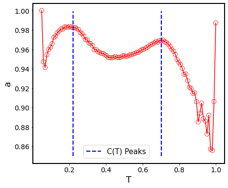
The key observation is the following: When is very large (i.e. higher than all the temperatures sampled in the Monte Carlo), all data, training and test, are labeled 0, and the neural net can learn that trivial labeling with 100% accuracy. The same is true for very small. Likewise, when arrives at a value close to the true transition temperature, the neural network will be able to classify most of the configurations correctly, yielding a very high accuracy. For other values of , the neural network will fail to distinguish some configurations from each other, resulting in comparatively low accuracies. It follows, then, that the accuracy vs temperature plots will have a ‘W’ shape, with the middle peak corresponding to the correct . In cases with two phase transitions, accuracy vs temperature plots result in a double ‘W’ shape, with the two peaks corresponding to the two critical temperatures. This process can also be done holding temperature constant, and varying other degrees of freedom such as .
Although the LBC method has had major success in recent years, it is important to note that, because we are using finite sized lattices, it is possible that the accuracy peak corresponds to a crossover rather than a true phase transition. While there is work indicating that the shape of the peak corresponds to the order of the phase transition Richter-Laskowska et al. (2022), it is still certainly possible that a peak corresponds to a crossover. As such, we turn to more traditional methods to more closely characterize the nature of the LBC accuracy peaks.
Traditionally, the LBC method is used with a fully connected neural network, which is expressive enough to distinguish phase transitions in many cases van Nieuwenburg et al. (2017); Lee and Kim (2019). In our case, however, such neural networks performed quite poorly, so convolutional neural networks (CNNs) were used instead, which are much better at picking out subtle spatial information from the data. It may be possible to get successful results with fully connected neural networks, but more data or a more complex training protocol may need to be used, slowing down the algorithm dramatically. Fig. 7 shows an example of the LBC method using CNNs, illustrating congruent results with traditional methods.
We tested the LBC approach on data generated from Monte Carlo simulations using , as it is sufficiently high for the existence of the sheet regime, but moving to larger values would increase the time for computation, as explained in the Appendix. We also tested the LBC scheme at many different values of to get more comprehensive results. As expected, LBC peaks and specific heat peaks were in strong agreement, both in cases with and without the sheet regime. Fig. 8 shows the resulting phase diagram generated from many runs similar to that of Fig. 7. In addition to sweeps across temperature, we also present multiple runs holding temperature constant, and sweeping across to further validate our results.
The use of the LBC approach applied to this model is not to claim superiority over traditional methods such as C(T) peaks, but rather to highlight its application to a specific problem in which the phase diagram was unknown. By benchmarking the LBC method in this way, we aim to show its effectiveness and reliability. The ultimate goal is to help expand the toolkit available for dealing with novel or poorly understood systems. In this way, we hope to underscore the potential of the LBC approach to provide new insights, which will become useful in areas where more traditional methods might face challenges.
VII Phase diagram
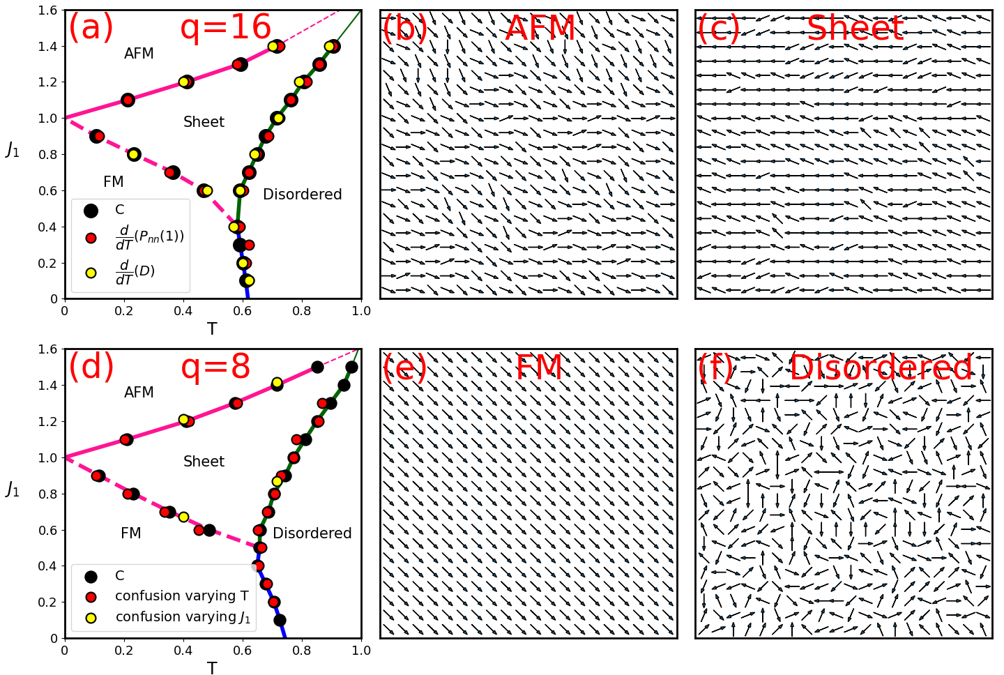
Based on the analysis in the above sections, we present in Fig. 8 the phase diagrams of our model for and , as well as snapshots of states in each of the phases. As we found in Sec. IV, and have qualitatively the same behavior, which is confirmed in panels (a) and (d). While there are slight differences in the specific transition temperatures, both phase diagrams have very similar structures. Lower values such as , however, are likely to yield much different phase diagrams, as is the case in the state clock model Ortiz et al. (2012).
At sufficiently low , the system stays at its FM or AFM ground states for and respectively, snapshots of which are also shown in Fig. 8. In the FM phase, all spins line up, whereas in the AFM phase, spins deviates by exactly one spin value from that of its neighbor’s, rendering a fluctuating-looking snapshot.
Below a critical value of ( for and for ), the system acts like a Potts model, which transitions into the disordered phase through a first order phase transition, as indicated by the blue line in the phase diagram. Increasing only slightly lowers , which can be understood since makes it harder for the system to develop ferromagnetic order.
Above the critical value of , as we increase , the system develops a sheet regime, before a phase transition into the disordered phase. A snapshot of the sheet regime is shown, where neighboring spins are able to take the same value as well as off-by-one values. For this reason, if we treat the spin values as a synthetic dimension, we’ll see a sheet in the 2 spatial + 1 synthetic dimension. For , the smooth transition in in Fig. 3 and the size independence of the peak in in Fig. 4 indicates that the boundary between the FM and sheet region is either a crossover or a KT transition. Similar size independence of heat capacity is observed in the model as well Nguyen and Boninsegni (2021). This is marked as a dashed magenta boundary in the phase diagrams. For , the transition from the AFM to the sheet region looks continuous as well if we look at the plot in Fig. 3. However, we believe it’s likely a second order phase transition as Fig. 4 shows clear size dependence of the heat capacity peak for , as opposed to . Furthermore, the FM and AFM phases are distinct, in that there should be a phase transition dividing the two regions. This provides further evidence that the boundary from the AFM phase to the sheet regime is a phase transition as opposed to a crossover. We have marked the phase boundary pink to differentiate from the first order transition happening between the FM and sheet phase.
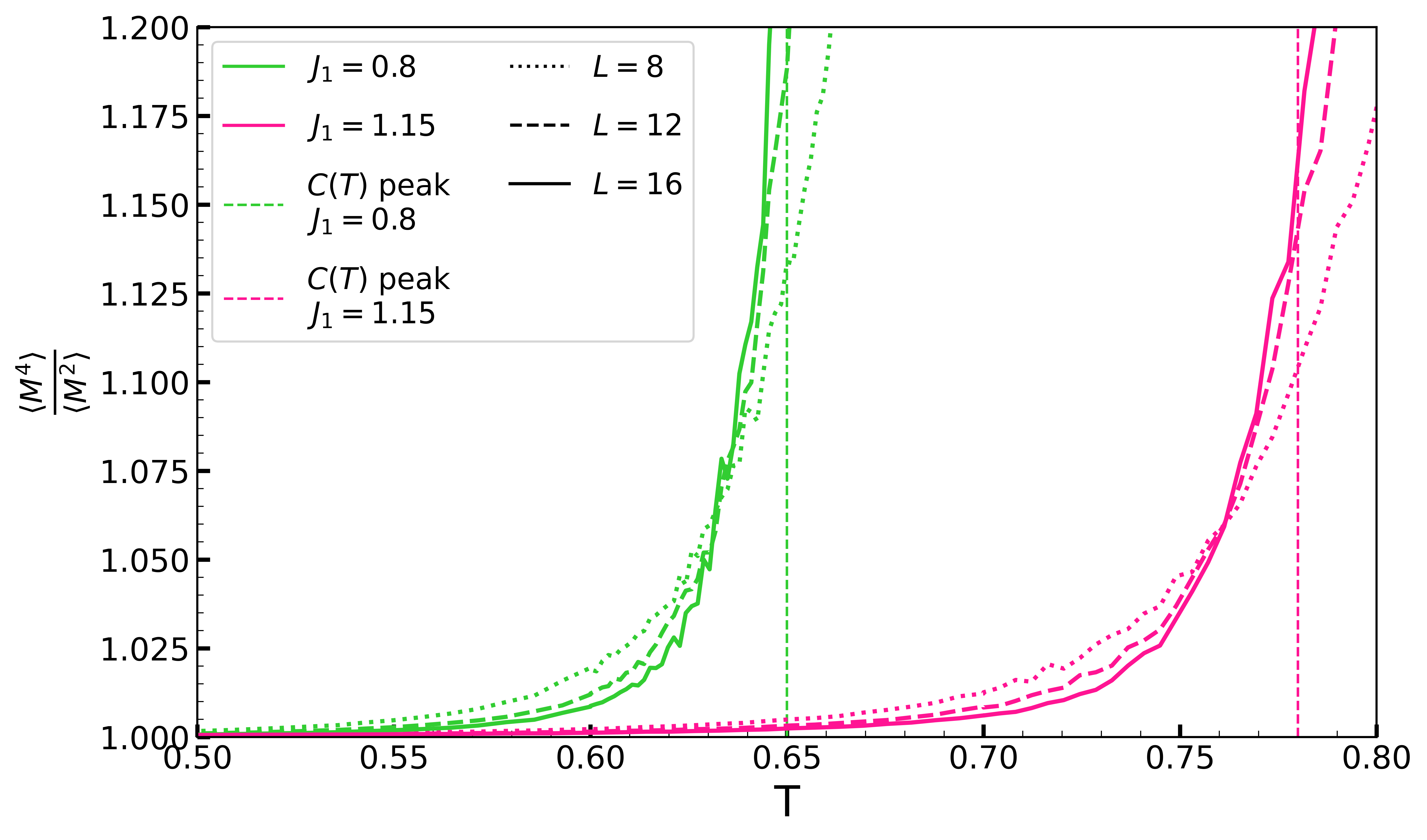
Finally for all , the system will eventually transition to a disordered phase through a second order phase transition, indicated by the green boundary in the phase diagram. We are be able to corroborate this claim while locating the transition temperature more accurately by using the Binder ratio . Here is defined as . It can be seen from Fig. 9 that the positions of the corresponding heat capacity peaks are very close to the critical temperatures indicated by the Binder ratio crossing points. However we should mention that the Binder ratio fails to capture other phase boundaries, thus we’re not showing the Binder ratio in a broader temperature range here.
VIII Conclusions
In this paper we have explored the phase diagram of a variant of the Potts model in which the energy is lowered not only when the degrees of freedom on adjacent spatial sites are identical, but where there is an additional energy lowering when they differ by , that is when . Such a situation mimics that of experiments with ultracold dipolar particles in synthetic dimensions, for example ultracold polar molecules in an optical trap in which each molecule has a ladder of possible rotational states with component of the angular momentum of molecule , and inter-molecular dipole interactions favor .
Although a precise connection between the two models is limited by the absence of quantum fluctuations in our classical analog, our results reveal several interesting qualitative links. In particular, we observe the emergence of a low temperature sheet regime which is very similar to one of the defining characteristics of the molecular system.
Prior studies Glumac and Uzelac (1998) of the three state Potts model have considered the effect of the range of the interaction on the order of the transition, finding first order character for . The context was that of a lattice with one (physical) dimension and long range (power law decaying) interactions. Our specific perspective here has been to formulate a classical model which serves as an analog of quantum models of sheet formation in synthetic dimension. Our work, which incorporates an energy which is lowered when adjacent sites (in two ‘physical’ dimensions) have variables which are identical (the usual Potts model) or differ by (our extension) can be interpreted as a similar extension of the ‘range’ of the interaction, but only in the third ‘synthetic’ direction.
Finally, we emphasize that determination of the phase diagrams of such models poses an interesting new challenge to machine learning and related information-theoretic Negrete et al. (2018, 2021) approaches being developed for statistical mechanics. We have shown here that learning by confusion van Nieuwenburg et al. (2017); Lee and Kim (2019) provides a powerful and accurate means to gain insight, and, significantly, that it is able to capture a ‘double-’ structure of the accuracy which might be expected in the presence of two successive finite temperature transitions.
IX Acknowledgements
M.C., Y.Z., M.C, and R.T.S acknowledge support from the U.S. Department of Energy, Office of Science, Office of Basic Energy Sciences, under Award Number DE-SC0022311. K.H. acknowledges support from the Welch Foundation (C-1872) and the National Science Foundation (PHY-1848304). K.H. thanks the Aspen Center for Physics, supported by the National Science Foundation grant PHY-1066293, and the KITP, supported in part by the National Science Foundation under Grant PHY-1748958, for their hospitality while part of this work was performed.
References
- Lin et al. (2016) Q. Lin, M. Xiao, L. Yuan, and S. Fan, “Photonic Weyl point in a two-dimensional resonator lattice with a synthetic frequency dimension,” Nature Communications 7, 1–7 (2016).
- Dutt et al. (2019) A. Dutt, M. Minkov, Q. Lin, L. Yuan, D. A. B. Miller, and S. Fan, “Experimental band structure spectroscopy along a synthetic dimension,” Nature Communications 10, 1–8 (2019).
- Kanungo et al. (2021) S. K. Kanungo, J. D. Whalen, Y. Lu, M. Yuan, S. Dasgupta, F. B. Dunning, K. R. A. Hazzard, and T. C. Killian, “Realizing Su-Schrieffer-Heeger topological edge states in Rydberg-atom synthetic dimensions,” arXiv preprint arXiv:2101.02871 (2021).
- Yuan et al. (2018) L. Yuan, Q. Lin, M. Xiao, and S. Fan, “Synthetic dimension in photonics,” Optica 5, 1396–1405 (2018).
- An et al. (2021) F. A. An, B. Sundar, J. Hou, X.-W. Luo, E. J. Meier, C. Zhang, K. R. A. Hazzard, and B. Gadway, “Nonlinear dynamics in a synthetic momentum-state lattice,” Phys. Rev. Lett. 127, 130401 (2021).
- Boada et al. (2012) O. Boada, A. Celi, J. I. Latorre, and M. Lewenstein, “Quantum simulation of an extra dimension,” Phys. Rev. Lett. 108, 133001 (2012).
- Ozawa and Price (2019) T. Ozawa and H. M. Price, “Topological quantum matter in synthetic dimensions,” Nature Reviews Physics 1, 349–357 (2019).
- Sundar et al. (2018) B. Sundar, B. Gadway, and K. R. A. Hazzard, “Synthetic dimensions in ultracold polar molecules,” Scientific reports 8, 1–7 (2018).
- Sundar et al. (2019) B. Sundar, M. Thibodeau, Z. Wang, B. Gadway, and K. R. A. Hazzard, “Strings of ultracold molecules in a synthetic dimension,” Physical Review A 99, 013624 (2019).
- Feng et al. (2022) C. Feng, K. Hazzard, and R. Scalettar, Physical Review A 105, 063320 (2022).
- Wu (1982) F. Y. Wu, “The Potts model,” Rev. Mod. Phys. 54, 235–268 (1982).
- Ortiz et al. (2012) G. Ortiz, E. Cobanera, and Z. Nussinov, “Dualities and the phase diagram of the p-clock model,” Nuclear Physics B 854, 780–814 (2012).
- Li et al. (2020) Z.-Q. Li, L.-P. Yang, Z. Y. Xie, H.-H. Tu, H.-J. Liao, and T. Xiang, “Critical properties of the two-dimensional -state clock model,” Phys. Rev. E 101, 060105 (2020).
- José et al. (1977) J. V. José, L. P. Kadanoff, S. Kirkpatrick, and D. R. Nelson, “Renormalization, vortices, and symmetry-breaking perturbations in the two-dimensional planar model,” Physical Review B 16, 1217 (1977).
- Cardy (1980) J. L. Cardy, “General discrete planar models in two dimensions: Duality properties and phase diagrams,” Journal of Physics A: Mathematical and General 13, 1507 (1980).
- Mittag and Stephen (1974) L. Mittag and M. J. Stephen, “Mean-field theory of the many component Potts model,” Journal of Physics A: Mathematical, Nuclear and General 7, L109 (1974).
- Wang (2016) L. Wang, “Discovering phase transitions with unsupervised learning,” Phys. Rev. B 94, 195105 (2016).
- Hu et al. (2017) W. Hu, R. R. P. Singh, and R. T. Scalettar, “Discovering phases, phase transitions, and crossovers through unsupervised machine learning: A critical examination,” Phys. Rev. E 95, 062122 (2017).
- Carrasquilla and Melko (2017) J. Carrasquilla and R. Melko, “Machine learning phases of matter,” Nature Physics 13, 431–434 (2017).
- Zhang et al. (2019) W. Zhang, J. Liu, and T.-C. Wei, “Machine learning of phase transitions in the percolation and XY models,” Physical Review E 99, 032142 (2019).
- Canabarro et al. (2019) A. Canabarro, F. Fanchini, A. Malvezzi, R. Pereira, and R. Chaves, “Unveiling phase transitions with machine learning,” Physical Review B 100, 045129 (2019).
- van Nieuwenburg et al. (2017) E. P. L. van Nieuwenburg, Y.-H. Liu, and S. D. Huber, “Learning phase transitions by confusion,” Nature Physics 13, 435–439 (2017).
- Lee and Kim (2019) S. Lee and B. Kim, “Confusion scheme in machine learning detects double phase transitions and quasi-long-range order,” Physical Review E 99, 043308 (2019).
- Tirelli et al. (2022) A. Tirelli, D. O. Carvalho, L. A. Oliveira, J. P. de Lima, N. C. Costa, and R. R. dos Santos, “Unsupervised machine learning approaches to the q-state Potts model,” The European Physical Journal B 95, 189 (2022).
- Richter-Laskowska et al. (2022) M. Richter-Laskowska, M. Kurpas, and M. Maśka, “A learning by confusion approach to characterize phase transitions,” arXiv preprint arXiv:2206.15114 (2022).
- Nguyen and Boninsegni (2021) P. H. Nguyen and M. Boninsegni, “Superfluid transition and specific heat of the 2D XY model: Monte carlo simulation,” Applied Sciences 11, 4931 (2021).
- Glumac and Uzelac (1998) Z. Glumac and K. Uzelac, “First-order transition in the one-dimensional three-state Potts model with long-range interactions,” Physical Review E 58, 4372 (1998).
- Negrete et al. (2018) O. A. Negrete, P. Vargas, F. J. Peña, G. Saravia, and E. E. Vogel, “Entropy and mutability for the q-state clock model in small systems,” Entropy 20 (2018), 10.3390/e20120933.
- Negrete et al. (2021) O. A. Negrete, P. Vargas, F. J. Peña, G. Saravia, and E. E. Vogel, “Short-range Berezinskii-Kosterlitz-Thouless phase characterization for the q-state clock model,” Entropy 23 (2021), 10.3390/e23081019.
Appendix: Classical Analog of Quantum Models in Synthetic Dimension
In this Appendix we consider details which provide additional insight into the model of Eq. 2 including (1) an evaluation of the ground state entropy, which we show to be extensive; and (2) details of the machine learning approach.
A. Macroscopic Ground State Entropy
When is dominant, there is a -fold degenerate ground state consisting of all sites sharing a common spin value. However, this degeneracy is ‘small’ in the sense that the entropy per site vanishes in the thermodynamic limit (i.e. fixed and large number of spatial sites ). One of the significant effects of is to introduce a macroscopic ground state degeneracy so that the associated low temperature entropy per site is non-zero. In particular, for on each bond the value of which minimizes the energy is not uniquely determined by , resulting in nonvanishing ground state entropy. Here we consider such entropy for a one dimensional chain of sites, focusing on the case when, on each bond, there are three choices which have equivalent energy. There is, however, a choice of boundary conditions in the synthetic dimension; we begin our analysis with periodic boundary conditions, followed by a discussion of open boundary conditions, which is easier to achieve in experiments.
With periodic boundary conditions in the synthetic dimension, the entropy for a one dimensional chain is easy to analyze analytically. We start with , looking at a single site, which can take different values. To keep the system in its ground state, all of its neighboring sites can each only take three different values: identical, one more, or one less. As more and more sites are considered, it becomes clear that each site—other than the first—can only take three different values. As such, in the limit as the number of sites goes to infinity, the degeneracy, and therefore entropy, can be written as,
For , a similar argument can be made, except each site is constrained only to take two possible values rather than three. Accordingly, in the limit as the number of sites goes to infinity, the entropy per site is found to be .
We now turn our attention to open boundary conditions in the synthetic dimension, which is substantially more difficult to analyze. Rather than calculating analytic expressions for the entropy, we establish lower and upper bounds, followed by computationally calculated approximations to check our results, all still for a one dimensional chain of sites. Starting with , one can use an analogous argument to the previous entropy calculations. With open boundary conditions, however, sites are constrained to take a maximum of three different values rather than strictly three different values. It is certainly possible that a site is constrained such that it can only take two or even one possible value (such as when the value of a neighboring site is 1 or ). Accordingly, in the limit as the number of sites goes to infinity, an upper bound to the ground state entropy per site is .
Still considering , to derive a lower bound we imagine a lattice in which every second site takes the same value. Given that so that this value can be neither the maximum or minimum ( or ), then each of the remaining sites is constrained to be either that same value, one more, or one less, resulting in a total of three different possibilities for each site. In the limit as the number of sites goes to infinity, the total number of microstates under this constraint and the ground state entropy per site can then be written as,
Since there are certainly other possible microstates, this is a lower bound for the ground state entropy per site. These upper and lower bounds hold in one dimension for any system size, and also for any . Similar arguments can be made for , resulting in lower and upper bounds of and respectively.
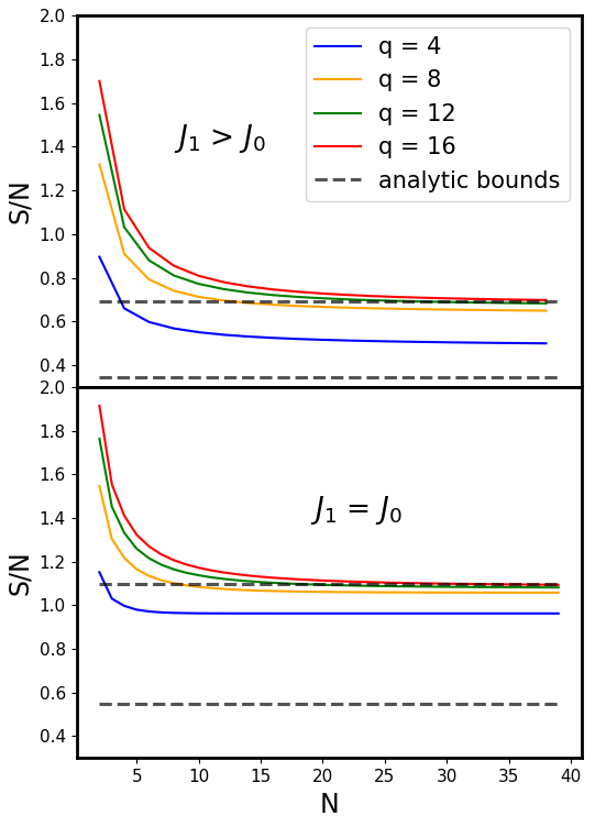
As mentioned previously, computational approximations for the ground state entropy are also calculated in one dimension for and . An algorithm was created using a Pascal’s triangle argument to count the number of microstates—and therefore entropy—for different chain sizes and values. This algorithm can best be understood by representing the one dimensional chain with a two dimensional grid of width and height , where the horizontal axis represents the position in the chain, and the vertical axis being the spin value of that particular site. For , the number of ground states is exactly given by the number of ways to travel from the left side to the right side of the grid while only making moves directly to the right, diagonally up/right, or diagonally down/right. Given periodic boundary conditions in the real dimension, the only other constraint is that there must be at most a one value difference between the starting and ending height positions on the grid. For the case, the same argument can be made, but only diagonal moves are allowed, and the ending height must be exactly one above or below the starting height. These types of questions, commonly known as pathway problems, are easily solved by creating an augmented Pascal’s Triangle starting from the far left of the grid, and propagating to the right by summing previous values along all available paths. Results are shown in Fig. S1. The best approximations are consistent with the previously established bounds.
B. Details of ML approach
As mentioned previously, we used the LBC method with CNNs. In particular, our CNNs consisted of 3 separate convolution layers in parallel with filter sizes , , and . After raw Monte Carlo configurations are put through each of these convolution layers, the outputs are then concatenated back into a single tensor, where the number of neurons is equal to the total number in the concatinated output of the CNNs. This tensor is then put through two fully connected layers with ReLU activation and 512 hidden neurons, finally running the two output neurons through softmax to classify the configuration into one of the two classes. A dropout probability of 0.1 was used in the fully connected layers to avoid overfitting.
Before each training trial, our data were split into training (42.5% of the data), testing (42.5% of the data), and validation (15% of the data) splits. The CNN is then trained using the training data split with Adam optimization, and cross-entropy loss on the validation split. Training ends once the validation loss stops decreasing for five epochs, which is done to avoid overfitting. The initial value of the learning rate is and is updated with Pytorch’s ReduceLROnPlateau learning rate scheduler, which multiplies the learning rate by a factor of 0.1 with a patience of 3. Accuracy is then calculated with the test data split, which is recorded so it can later be plotted.
Our data sets consisted of independent configurations at different temperatures, resulting in total configurations. When temperatures are sufficiently low, however, the sampling is not ergodic and the simulation spends a very long time in one of the degenerate ordered states. To address this, ‘spatially translated’ data were created as follows: From each ‘real’ configuration, ‘translated’ configurations were generated by increasing the spin value on each site: , with PBC imposed such that , This corresponds to moving the configuration in the synthetic dimension. Likewise all spatial sites are also translated a random amount in the two ‘real’ dimensions. These two steps were performed times, resulting in different configurations with the same energy as the original. The final data set consists of total configurations. Accordingly, higher values result in larger amounts of translated data, thus increasing computation time.