Classical crystal formation of dipoles in two dimensions

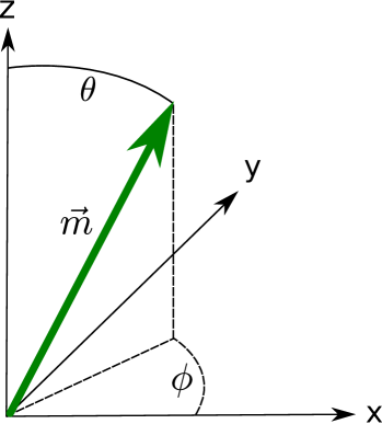
All dipoles are assumed to be identical with a given dipole moment of size $D$. They all have the same orientation induced by the application of an external magnetic or electric field. The direction of the dipole moments is given by the angles $(\theta$, $\phi$) as illustrated in Fig. 1. The dipole moment itself, $\vec{m}$ is then described by

The interaction energy between two of these dipoles, $\vec{m}_{1}$ and $\vec{m}_{2}$, is

where $\vec{r}$ is the vector between the two dipoles, $r=|\vec{r}|$, and $C=\tfrac{\mu_{0}}{4\pi}$ and $C=\tfrac{1}{4\pi\epsilon_{0}}$ for magnetic and electric dipoles, respectively. Here $\mu_{0}$ and $\epsilon_{0}$ are the vacuum permeability and vacuum permittivity, respectively. Below we will assume magnetic dipoles. Results for electric dipoles can be obtained by simply making the substitution $\mu_{0}\to 1/\epsilon_{0}$.

We now assume that the two dipoles are placed on the $x$-axis at a distance $r$ and described by the angles $\theta$ and $\phi$. For identical dipole moments $(\vec{m}_{1}=\vec{m}_{2})=\vec{m}$ the potential energy in Fig. 2 is reduced to

since $\vec{r}$ is taken along the $x$-axis. We thus see that the interaction energy is positive as long as

We therefore conclude that the interaction is repulsive for all $\phi$ when $\theta<\theta_{c}\equiv\sin^{-1}\left(1/\sqrt{3}\right)=0.61548$. Thus, collapse due to attractive inverse cubic interactions can not occur for $\theta<0.61548$. We note that the $\sin^{2}\theta$ dependence implies a symmetry around $\theta=\pi/2$ corresponding to reflection in the $xy$-plane where all dipoles are assumed to be located.

When comparing different crystal structures we must consider the conditions we impose on the system. We imagine that the crystal forms from a gas phase that condenses by cooling. Consequently the crystal structures most likely prefer to have a constant density of dipoles in the plane, i.e. we do not have clumping or holes in the crystal. We thus assume an ideal uniform crystal structure. It is of course very interesting to study the effect of crystal defects in both a classical and quantum mechanical setting but this is beyond the scope of the present study.

We therefore aim at determining the preferred regular crystal structure for a given alignment of the many dipole moments distributed to produce a given average density in the $xy$-plane. We then need to find the configuration that minimizes the total interaction energy for such specification of the system. The total interaction energy, $U$, is

where $\vec{R}$ and $\vec{R^{\prime}}$ are position vectors of each pair of dipoles interacting through the potential, $I(\vec{r})$, in Eq. (2).

We need a sensible unit cell that can be used to parametrize the crystal structure for given external alignment. An important limit to consider is the one of perpendicular dipoles, i.e. when all the dipole moments are aligned perpendicular ($\theta=0$) to the plane containing all the particles. In this case the dipole-dipole interaction is purely repulsive with a $r^{-3}$ behavior that only depends on the relative distance. The system will try to maximize the distance between each pair of dipoles and not allow any clusterization or irregular correlations (at least in the ideal crystal we investigate). Finding the minimum energy configuration for this system is therefore the same problem as the packing of spheres. This problem is known to have a hexagonal solution in 2D faststof2 and we therefore must be able to capture this geometry with our unit cell parametrization.

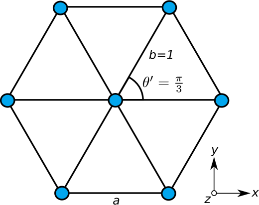
To allow sufficient flexibility we choose the unit cell shown in Fig. 3. The two variables $\theta$’ and $b$ allow us to describe all uniform crystal structures with $a$ as the crystal lattice length. Symmetry allows a restriction of $\theta$’ to the interval $[0,\pi/2[$ and $b$ to be less than unity, i.e. $]0,1]$. The value of $a$ can be determined as function of $\theta$’ and $b$ to maintain a given average density of dipoles in the resulting crystal. This can be imposed by insisting that the unit cell area remains constant as we change the parameters $\theta^{\prime}$ and $b$. The density, $\sigma$, is inversely proportional to the area, $a^{2}b\sin\theta^{\prime}$, of the unit cell. The constraint on $a$ is then

The two unit cell basis vectors, $a_{i}$, connecting nearest neighbors in the two principal directions are

We may now exploit the symmetries of the unit cell. As mentioned before there is a symmetry around $\theta=\pi/2$. There is also a symmetry resulting in $U\left(\phi\right)=U\left(\phi+\pi\right)$ where the energy is invariant under translation of $\phi$ by $\pi$. This can easily be seen by the invariance of rotating the unit cell 180 degrees around the $z$-axis, e.g. rotating around the central point in Fig. 3. It can also be seen by looking at the expression for the dipole interaction in Eq. (3). The dependence on $\phi$ goes as $\cos^{2}\phi$ and this is invariant under rotations by $\pi$. We can therefore reduce the parameter space and work with $\theta\in[0,\pi/2]$ and $\phi\in[0,\pi]$.

It is important to note that the external alignment of the dipoles fixes $\theta$ as the angle between the $z$-axis and the direction of the external electric or magnetic field. The other angle, $\phi$, describes the angle between the arbitrarily chosen $x$-axis of the unit cell and the projection on the crystal plane of the aligned dipole moments. The calculational procedure will therefore be to fix $\theta$ and $\phi$, and then minimize the energy with respect to $\theta^{\prime}$ and $b$. This will for each $\theta$ produce an energy as a function of $\phi$ and the minimum will then define the preferred crystal structure for this given $\theta$.

In general a complicated topology may invalidate this procedure of fixing one parameter, minimizing with respect to two other parameters, and afterwards find minimum of the resulting function of the first parameter. All three variables should perhaps be varied simultaneously to find true global or local minima. To confirm that our procedure provided correct minima we tested by numerical variation of the parameters around the minima.

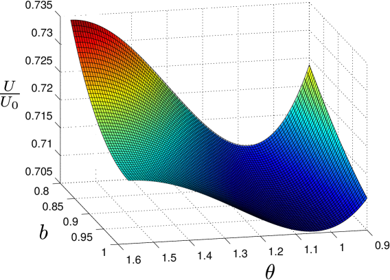
First we consider the structures arising for $\theta=0$ where the dependence on $\phi$ drops out. It is indeed the simplest case yet it is a relevant benchmark to demonstrate the validity of our method. The total interaction energy from Eq. (5) as a function of $\theta^{\prime}$ and $b$ is shown in Fig. 4. Energies are plotted in units of $U_{0}=\mu_{0}D^{2}\sigma^{3/2}$ where the density of dipoles, $\sigma$, is kept constant in all calculations.

As expected, we find that the minimum in energy occurs when $\theta^{\prime}=\pi/3$ and $b=1$. The unit cell of the corresponding hexagonal lattice structure of lowest energy is shown in Fig. 5. Note that for $\theta=0$ there is a triangular symmetry which is the result of the rotational symmetry in the plane for $\theta=0$ which is broken down to the point-group symmetry of the hexagonal lattice when the crystal forms.

A rather flat valley extends in Fig. 4 from the minimum in the direction of smaller $b$ for fixed $\theta^{\prime}=\pi/3$. The walls increase rather steeply on both sides of this valley. The crystal is therefore relatively soft towards moving the upper (and lower) dipoles in Fig. 5 further away from (or closer to) each other and the central line of dipoles along the direction of $\theta^{\prime}=\pi/3$. We emphasize that precisely the same unit cell is obtained for $\theta^{\prime}=2\pi/3$. Consequently a similar minimum would show up by extending Fig. 4 to larger values of $\theta^{\prime}$. The barrier between the two minima is already indicated and almost reached. No other direction parametrized by $\theta^{\prime}$ provide the same structure for the same density.

Small changes of $\theta$ away from zero would break the hexagonal lattice symmetry and introduce a preferred direction connected to the direction of the external field that aligns the dipoles. The soft directions along $\theta^{\prime}=\pi/3$ and $\theta^{\prime}=2\pi/3$ then must be either followed or overpowered. The hexagonal structure must be distorted or completely changed.

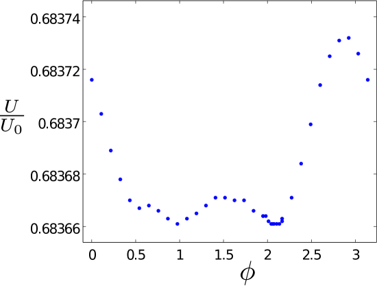
We now move the polarization direction, $\theta$, away from being perpendicular to the crystal plane. The crystal has to adjust by finding the minimum energy with respect to $b$, $\theta^{\prime}$, and $\phi$. For convenience we minimize with respect to $b$ and $\theta^{\prime}$ for each value of $\phi$. The resulting functions are shown in Fig. 6 for three different values of $\theta$.

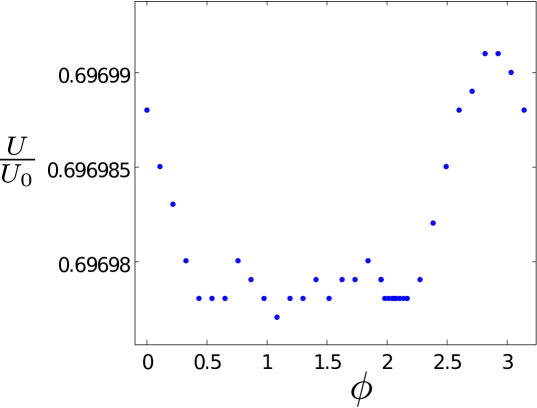
The energy for the smallest polarization angle, $\theta=0.1$, is exhibited in the upper panel. The variation with $\phi$ is exceedingly small with a decrease from the $\theta=0$ result of $0.7072$ by around $1\%$.

The case of small angle polarization is nevertheless the first step away from the highest symmetry and towards collapse of the crystal structure. The case of $\theta=0.1$ in Fig. 6 already exhibits all the tendencies to develop pronounced minima in the potential energy surface. We observe the global minimum at $\phi=1.083$, which corresponds to $\theta^{\prime}=1.056$ and $b=0.99$. The structure for this minimum is then visualized as a polarization direction, $\phi$, tilted in the direction of $\theta^{\prime}=\pi/3$.

We also note additional (local) minima around $\phi=2.058$ and $\phi=0.542$. The first of these corresponds to a structure with $\phi=\theta^{\prime}=2\pi/3$, that is the same geometry as the global minimum but for a different unit cell. The second minimum corresponds to $\phi\approx\pi/6$, $\theta^{\prime}\approx\pi/3$, and $b\approx 0.99$, that is an apparently metastable structure. We emphasize that all minima are tested to be real minima by direct computation of the energy surface in a cubic grid around the minimum points. In any case the energy differences are very small and sometimes at the limit of being significant.

Still it is of interest to understand the emerging structures. The minimum energy configuration for $\phi=0.542$ is the same as for the two deeper minima but now the polarization direction is half way between those of the preferred global minimum, $\phi\approx\theta^{\prime}=\pi/3$, and the extreme linear structure, $\phi\approx\theta^{\prime}=0$. The symmetry is very high as the polarization points directly to towards the opposite, furthest away, dipole in the unit cell.

Going away from the flat region for intermediate $\phi$-values, both towards smaller and larger values of $\phi$ we find a steeply increasing energy. The curve beyond $\phi=\pi$ continues precisely as for $\phi=0$. The maximum is relatively high and associated with a structure corresponding to the hexagonal structure which is energetically unfavored.

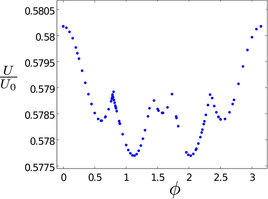
Tilting the dipole to $\theta=0.15$ leads to larger variation of the potential energy as shown in the middle part of Fig. 6. The deepest minimum associated with the optimal crystal structure still appears for about the same structure values, $\phi=2.058$, $\theta^{\prime}=1.025$ and $b=1$, as for $\theta=0.1$. The minimum with the same crystal structure for about $\phi=0.975$, $\theta^{\prime}=1.067$ and $b=0.98$ is fortunately also found with the same energy. The overall features in the energy as function $\phi$ remain the same as for $\theta=0.1$ but now determined with better relative accuracy. The local minimum at about $\phi\approx 0.542$ has almost disappeared.

Proceeding to the larger polarization angle of $\theta=0.35$ we find the energy shown in the lower part of Fig. 6. The two optimal minima are now rather pronounced at the same $\phi$-values of $\phi=2.028$ and $1.133$. The two local minima at about $\phi=0.600$ and $2.500$ are now clearly seen in the figure. They correspond to crystal structures described by $\theta^{\prime}\approx 1$ and $b\approx 0.35$. These local minima are sensitive to the influence from dipoles at very large distances which tend to increase the minimum values and perhaps eventually wipe them out completely.

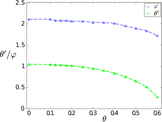
The minimum energy configurations for the different $\theta$-values all correspond to $b\approx 1$. The variations of $\theta^{\prime}$ and $\phi$ as functions of $\theta$ are shown in Fig. 7. The similarity is striking as the two equivalent minima correspond to $\phi\approx\theta^{\prime}$ and $\phi\approx 2\theta^{\prime}$. As already mentioned this is not surprising as the same structure arises and the polarization direction points along the highest symmetry axis of the crystal structure.

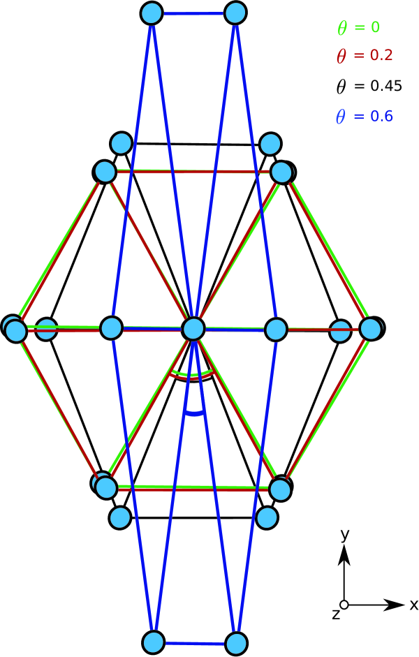
The two identical optimal structure changes systematically with $\theta$ as illustrated in Fig. 8. It is seen clearly that the structure evolves continuously from the hexagonal structure in Fig. 5 and towards lines of well separated dipoles. The ultimate linear configurations place the dipoles at pairwise minimum energy positions with respect to each other.

The change in structure seems to be accelerating as $\theta$ becomes larger and approaching the structure where each row of dipoles would collapse on itself after crossing the threshold into the range of inverse cubic attraction at zero distance. This configuration is very near the point $\theta_{c}=0.615$ where attraction between two dipoles would occur, and it would seem logical that this is the point where the structure would collapse. The last configuration we investigated was for $\theta=0.6$ where the angle $\theta^{\prime}$ is approaching the dive down towards zero as seen in in Fig. 7.

The overall change in the system makes sense intuitively. As the dipole-interaction weakens as $\theta$ grows it makes sense that the dipoles would try to place themselves behind each other at the minimum energy positions with the nearest neighbours. The more it weakens the more favourable this positioning becomes and the structure will change accordingly.

The interaction energy is calculated by use of Eqs. (2) and (5) for a given equilibrium structure where the dipoles are located at a series of lattice points, $\vec{R}_{0}$. We move the dipoles a small distance away from their respective equilibrium positions, $\vec{u}(\vec{R}_{0})$, such that $\vec{R}=\vec{R}_{0}+\vec{u}(\vec{R}_{0})$. Then change of the pairwise distance becomes $\vec{\delta u}=\vec{u}(\vec{R}_{0})-\vec{u}(\vec{R}^{\prime}_{0})$ which assumed small allows expansion of the energy in Eq. (5) to second order in $\vec{\delta u}$. The zeroth order term will not contribute to the dynamics. The first order term will vanish as we expand around minimum positions.

We now assume equilibrium at $\vec{R}$ and omit from now on the index, ${}^{\prime\prime}0^{\prime\prime}$. The gradient of the second order term provides the force on the amplitude, $\vec{u}$, and the equation of motion becomes

where $M$ is the mass of one dipole, and the elements of the $D$-matrix are defined by

We search for periodic solutions, $\vec{u}(\vec{R})$, in a direction described by the unit vector, $\vec{\epsilon}$, by inserting the ansatz,

into Eq. (8) for a constant given wave vector, $\vec{k}$. The resulting two-dimensional eigenvalue equation gives us two solutions corresponding to vibrational frequencies, $\omega(\vec{k})$, and related to the two normal mode directions, $\vec{\epsilon}$, parallel and perpendicular to the wave vector, $\vec{k}$.

From the eigen frequencies determined for the central symmetry point, $\Gamma$ in Fig. 9, we calculate the corresponding sound velocities,

for the two normal modes, transverse and longitudinal waves.

To analyze the phonon spectrum we need to know the points of interest in the reciprocal lattice. We therefore calculate the reciprocal lattice as a function of $\theta^{\prime}$ and $b$. We define $\vec{b}_{1}$ an $\vec{b}_{2}$ as the reciprocal lattice vectors. From the definition of reciprocal lattice vectors we have

where $\vec{a}_{i}$ are the lattice vectors in Eq.(7). This leads to:

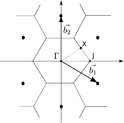
The symmetric structure of $\theta^{\prime}=\frac{\pi}{3}$ and $b=1$ shown in Fig. 5 then corresponds to the reciprocal lattice in the upper part of Fig. 9. Three different symmetry points are immediately recognized and marked by $\Gamma$, X and J in the figure. They are respectively the point $(0,0)$, the point between the two dipoles at $(0,0)$ and $\vec{b}_{1}+\vec{b}_{2}$, and the corner between three Brillouin zones for the dipoles at $(0,0)$, $\vec{b}_{1}$ and $\vec{b}_{1}+\vec{b}_{2}$.

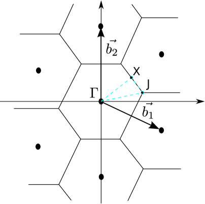
Increasing the value of $\theta^{\prime}$ above $\pi/3$ moves the $\vec{b}_{1}$-vector closer to the $x$-axis. This results in a twisting of the reciprocal lattice as shown in lower part of Fig. 9. The symmetry points, $\Gamma$, X and J, for the perpendicular dipoles solution are also present for all other values of $b$ and $\theta^{\prime}$. Decreasing $\theta^{\prime}$ would lead to a twisting of the reciprocal lattice in the opposite direction of going from upper to lower part of Fig. 9.

These symmetry points will be natural target points for the wave vector in investigations of the phonon spectra of the different structures.

The phonon spectra are calculated along the closed path passing through symmetry points $\Gamma$, $X$ and $J$ shown in upper panel on Fig. 9. The wave vector, $\vec{k}$, always begins at the origin, $\Gamma$. First it increases in size in the direction of $X$, then it follows the line towards $J$, and finally it maintains this direction while decreasing size until zero at the starting point, $\Gamma$.

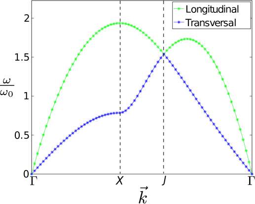
The phonon spectrum is then calculated and shown in Fig. 10 for perpendicular dipoles of $\theta=0$. Two frequencies arise from diagonalizing the $2\times 2$ $D$-matrix. The two types of vibrations are denoted longitudinal and transverse corresponding to small amplitude motion of all dipoles along and perpendicular to the $\vec{k}$-direction, respectively.

The two computed frequencies both increase from zero at the symmetry point, $\Gamma$. The longitudinal mode show the fastest increase of energy, reaching a maximum at the edge of the Brillouin zone, when the wave vector reaches its maximum at the symmetry point $X$. The transverse frequency increases slower but with a similar flat region before reaching $X$.

With the wave vector end-point continuing from $X$ towards $J$ we find a smoothly decreasing longitudinal frequency and a more abruptly, yet continuously, increasing transversal frequency.

As the symmetry point, $J$, for the hexagonal lattice is approached the two frequencies meet each other in one degenerate value. As this is a highly symmetrical point for the hexagonal lattice such a behavior would be expected here but it is also only expected for this particular case.

The two frequency curves continue smoothly through this point, but interchange correspondingly vibrational character between transversal and longitudinal mode. The longitudinal mode continues to reach a maximum before decreasing towards zero at $\Gamma$, while the transversal mode decreases directly towards zero at the central point.

Both frequencies approach zero at the symmetry point, $\Gamma$, although with different rates. Thus no optical branch is found in agreement with what is expected for a single particle basis.

We now slowly increase $\theta$ above zero. For small values the structure is rather similar to that of $\theta=0$. Accordingly the changes in the phonon spectrum is small although noticeable. The complete hexagonal symmetry is broken and a $\phi$-dependence of the interaction energy appear for finite values of $\theta$, see Fig. 6. The symmetry is no longer perfect even for a small value of $\theta=0.1$, but the symmetry points remains in the reciprocal lattice sketched in Fig. 9. The degeneracy in the point $J$ is lifted and the two branches begin to move away from each other at this point.

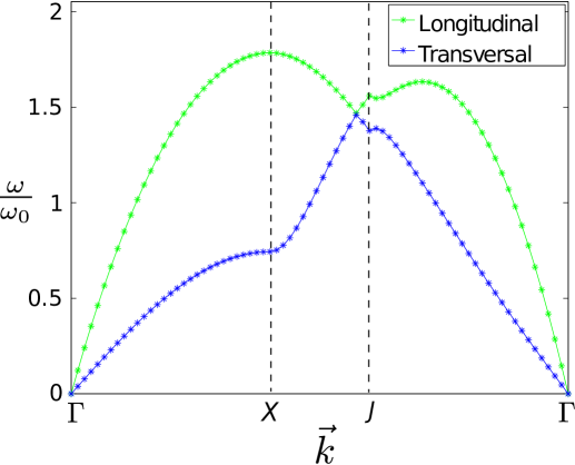
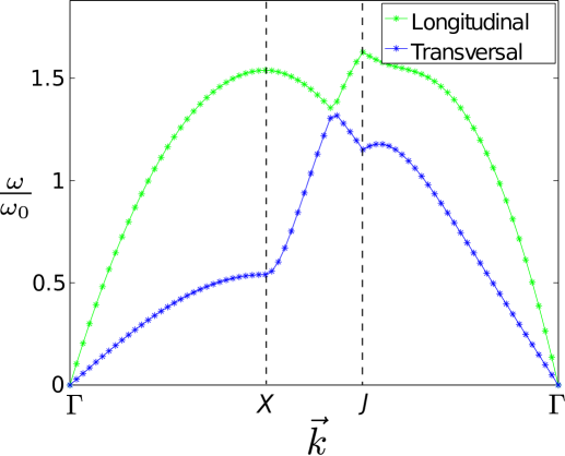
Increasing $\theta$ changes the structure substantially especially towards the critical value $\theta_{c}$. The results for increasing $\theta$ are shown in Fig. 11 for three larger illustrative values. For $\theta=0.25$ the degeneracy at point $J$ has now clearly disappeared and a significant gap has appeared. The spectrum still maintain the same features and the same overall appearance. However, now a small minimum appears on the longitudinal branch close to the point $J$. This minimum is present for all spectra in the interval from $\theta=0.2-0.35$. After appearance it first becomes deeper but as $\theta$ grows so does the frequency at $J$ and for $\theta=0.35$ the minimum is altogether washed out. The significance of this minimum could possible be a signal of roton dynamics in the crystal in analogy to that of helium helium . Such rotons have been predicted and discussed also for particles with dipolar interactions mazzanti2009 ; hufnagl2011 ; zinner2012 ; macia2012 ; bisset2013 ; fedorov2014a ; fedorov2014b . It is clearly related to deformation of the crystal, but we postpone more detailed investigations to future work.

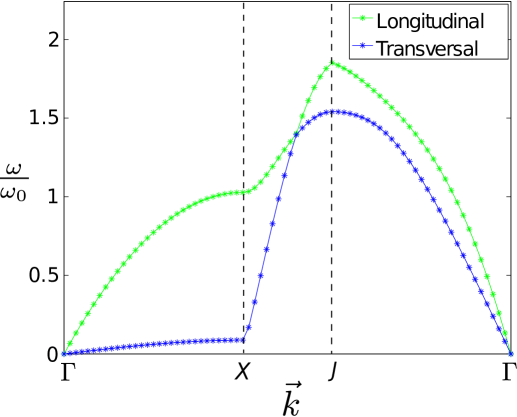
Increasing $\theta$ to $0.4$ and beyond, we see that the spectra in Fig. 11 change appearance. The point $X$ moves closer to $\Gamma$ in Fig. 9. We note that no new minima appear beside the kink at $J$ in the transversal frequency for $\theta=0.4$. The spectrum for $\theta=0.55$ is apparently more distorted with kinks or abruptly changing values. However, we emphasize that the $x$-axes on Fig. 11 do not reflect real distances. It is merely the result of the choice of discrete wave vectors $\vec{k}$, and the subsequent distance between points on the figures. Therefore the variation is not a realistic signal representative for any physical effect.

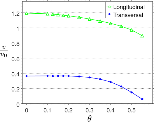
With the phonon spectrum available we calculate the speed of sound, $v$, from Eq. (11) in the point, $\Gamma$, in both transverse and longitudinal directions. The results are seen to be the derivatives of the frequency curves in Figs. 10 and 11. Each configuration then has longitudinal and transversal values for the speed of sound as shown in in Fig. 12 as functions of $\theta$. For the hexagonal structure, $\theta=0$, we find $v=1.19481v_{0}$ and $v=0.364272v_{0}$, respectively, in the natural units of $v_{0}=\sqrt{\frac{D^{2}\mu_{0}\sigma^{3/2}}{M}}$.

Both longitudinal and transversal velocities decrease continuously and relatively slowly with $\theta$. There is a tendency to speed up the reduction as the critical polarization angle is approached. This is intuitively understandable, since the structure for $\theta\rightarrow\theta_{c}$ approaches separated straight lines as seen in Fig. 8. The frequencies decrease when the instability is approached, and correspondingly the speed of sound must decrease. This instability in also clear to see in bottom panel of Fig. 11 where we see the normal mode going towards zero energy at the point $X$.

References

- (1) S. Ospelkaus et al., Nature Phys. 4, 622 (2008);
- (2) K.-K. Ni et al., Science 322, 231 (2008);
- (3) J. Deiglmayr et al., Phys. Rev. Lett. 101, 133004 (2008);
- (4) F. Lang et al., Phys. Rev. Lett. 101, 133005 (2008);
- (5) D. Wang et al., Phys. Rev. A 81, 061404(R) (2010);
- (6) B. C. Sawyer et al., Phys. Chem. Chem. Phys. 13, 19059 (2011)
- (7) K-.K. Ni et al., Nature 464 1324, (2010)
- (8) S. Ospelkaus et al., Science 327 853, (2010)
- (9) M. G. H. de Miranda et al., Nature Phys. 7, 502 (2011)
- (10) B. Yan et al., Nature 501, 521 (2013)
- (11) B. Zhu et al., Phys. Rev. Lett. 112, 070404 (2014)
- (12) K. Aikawa et al., Phys. Rev. Lett. 113, 263201 (2014)
- (13) T. Takekoshi et al., Phys. Rev. Lett. 113, 205301 (2014)
- (14) P. M. Lushnikov, Phys. Rev. A 66, 051601 (2002)
- (15) A. Micheli, Z. Idziaszek, G. Pupillo, M. A. Baranov, P. Zoller, and P. S. Julienne, Phys. Rev. Lett. 105, 073202 (2010)
- (16) S.-M. Shih and D.-W. Wang, Phys. Rev. A 79, 065603 (2009);
- (17) D. V. Fedorov, J. R. Armstrong, N. T. Zinner, and A. S. Jensen, Few-body Syst. 50, 417 (2011);
- (18) M. Klawunn, A. Pikovski, and L. Santos, Phys. Rev. A 82, 044701 (2010);
- (19) A. G. Volosniev, D. V. Fedorov, A. S. Jensen, and N. T. Zinner, Phys. Rev. A 85, 023609 (2012)
- (20) J. C. Cremon, G. M. Bruun, and S. M. Reimann, Phys. Rev. Lett. 105, 255301 (2010)
- (21) S. Zöllner, Phys. Rev. A 84, 063619 (2011)
- (22) N. T. Zinner, J. R. Armstrong, A. G. Volosniev, D. V. Fedorov, and A. S. Jensen, Few-Body Syst. 53, 369 (2012)
- (23) S.-J. Huang et al., Phys. Rev. A 85, 055601 (2012)
- (24) A. G. Volosniev, J. R. Armstrong, D. V. Fedorov, A. S. Jensen, M. Valiente and N. T. Zinner, New J. Phys. 15, 043046 (2013)
- (25) K. Góral, L. Santos, and M. Lewenstein, Phys. Rev. Lett. 88, 170406 (2002);
- (26) D. DeMille, Phys. Rev. Lett. 88, 069701 (2002);
- (27) R. Barnett, D. Petrov, M. Lukin, and E. Demler, Phys. Rev. Lett. 96, 190401 (2006);
- (28) A. Micheli, G. K. Brennen, and P. Zoller, Nature Phys. 2, 341 (2006).
- (29) D.-W. Wang, M. D. Lukin, and E. Demler, Phys. Rev. Lett. 97, 180413 (2006)
- (30) G. M. Bruun and E. Taylor, Phys. Rev. Lett. 101, 245301 (2008);
- (31) R. M. Lutchyn, E. Rossi, and S. Das Sarma, Phys. Rev. A 82, 061604(R) (2009);
- (32) Y. Yamaguchi, T. Sogo, T. Ito, and T. Miyakawa, Phys. Rev. A 82, 013643 (2010);
- (33) A. Pikovski, M. Klawunn, G. V. Shlyapnikov, and L. Santos, Phys. Rev. Lett. 105, 215302 (2010);
- (34) F. Herrera, M. Litinskaya, R. V. Krems, Phys. Rev. A 82, 033428 (2010);
- (35) L. Pollet, J. D. Picon, H. P. Büchler, and M. Troyer, Phys. Rev. Lett. 104 125302 (2010);
- (36) J. Levinsen, N. R. Cooper, and G. V. Shlyapnikov, Phys. Rev. A 84, 013603 (2011);
- (37) L. He, W. Hofstetter, Phys. Rev. A 83, 053629 (2011)
- (38) J. K. Block, N. T. Zinner and G. M. Bruun, New J. Phys. 14, 105006 (2012);
- (39) L. D. Carr, D. DeMille, R. V. Krems, and J. Ye, New J. Phys. 11, 055049 (2009)
- (40) M. A. Baranov, Phys. Rep. 464, 71 (2008);
- (41) T. Lahaye, C. Menotti, L. Santos, M. Lewenstein, and T. Pfau, Rep. Prog. Phys. 72, 126401 (2009)
- (42) P. K. Molony et al., Phys. Rev. Lett. 113, 255301 (2014)
- (43) T. Shimasaki et al., Phys. Rev. 91, 021401(R) (2015)
- (44) E. Wigner, Phys. Rev. 46, 1002 (1934)
- (45) L. Bonsall and A. A. Maradudin, Phys. Rev. B 15, 1959 (1977)
- (46) R. K. Kalia and P. Vashishta, J. Phys. C 14, L643 (1981)
- (47) V. M. Bedanov, G. V. Gadiyak, Yu. E. Lozovik, JETP 61, 967 (1985)
- (48) B. Groh and S. Dietrich, Phys. Rev. E 63, 021203 (2001).
- (49) X. Lu, C.-Q. Wu, A. Micheli, and G. Pupillo, Phys. Rev. B 78, 024108 (2008)
- (50) I. R. O. Ramos, W. P. Ferreira, F. F. Munarin, G. A. Farias, and F. M. Peeters, Phys. Rev. E 85, 051404 (2012)
- (51) C. Mora, O. Parcollet, and X. Waintal, Phys. Rev. B 76, 064511 (2007);
- (52) H. P. Büchler et al., Phys. Rev. Lett. 98, 060404 (2007);
- (53) G. E. Astrakharchik, J. Boronat, I. L. Kurbakov, and Yu. E. Lozovik, Phys. Rev. Lett. 98, 060405 (2007)
- (54) N. Matveeva and S. Giorgini, Phys. Rev. Lett. 109, 200401 (2012)
- (55) S. Moroni and M. Boninsegni, Phys. Rev. Lett. 113, 240407 (2014)
- (56) A. Macia, G. E. Astrakharchik, F. Mazzanti, S. Giorgini, and J. Boronat, Phys. Rev. A 90, 043623 (2014)
- (57) J. Quintanilla, S. T. Carr, and J. J. Betouras, Phys. Rev. A 79, 031601(R) (2009);
- (58) S. T. Carr, J. Quintanilla, and J. J. Betouras, Phys. Rev. B 82, 045110 (2010)
- (59) B. Capogrosso-Sansone, C. Trefzger, M. Lewenstein, P. Zoller, and G. Pupillo, Phys. Rev. Lett. 104, 125301 (2010)
- (60) A.-L. Gadsbølle and G. M. Bruun, Phys. Rev. A 85, 021604(R) (2012)
- (61) K. Sun, C. Wu, and S. Das Sarma, Phys. Rev. B 82, 075105 (2010);
- (62) N. T. Zinner and G. M. Bruun, Eur. Phys. J. D 65, 133 (2011)
- (63) M. M. Parish and F. M. Marchetti, Phys. Rev. Lett. 108, 145304 (2012)
- (64) M. Plischke and B. Bergersen, Equilibrium Statistical Physics, (World Scientific, London, 2nd ed., 2006).
- (65) V. A. Froltsov, R. Blaak, C. N. Likos, and H. Löwen, Phys. Rev. E 68, 061406 (2003)
- (66) V. A. Froltsov et al., Phys. Rev. E 71, 031404 (2005)
- (67) F. Lindemann, Physik Z. 11, 609 (1910)
- (68) P. M. Chaikin and T. C. Lubensky, Principles of Condensed Matter Physics (Cambridge University Press, Cambridge, 1995)
- (69) B. I. Halperin and D. R. Nelson, Phys. Rev. Lett. 41, 121 (1978)
- (70) G. M. Bruun and D. R. Nelson, Phys. Rev. B 89, 094112 (2014)
- (71) D. R. Nelson and B. I. Halperin, Phys. Rev. B 19, 2457 (1979)
- (72) N. W. Ashcroft and N. D. Mermin, Solid State Physics, (Harcourt, Orlando, 1st ed., 1976).
- (73) F. Mazzanti, R. E. Zillich, G. E. Astrakharchik, and J. Boronat, Phys. Rev. Lett. 102, 110405 (2009).
- (74) D. Hufnagl, R. Kaltseis, V. Apaja, and R. E. Zillich, Phys. Rev. Lett. 107, 065303 (2011).
- (75) N. T. Zinner, B. Wunsch, D. Pekker, and D.-W. Wang, Phys. Rev. A 85, 013603 (2012);
- (76) A. Macia, D. Hufnagl, F. Mazzanti, J. Boronat, and R. E. Zillich, Phys. Rev. Lett. 109, 235307 (2012).
- (77) R. N. Bisset and P. B. Blakie, Phys. Rev. Lett. 110, 265301 (2013).
- (78) A. K. Fedorov, I. L. Kurbakov, and Yu E. Lozovik, Phys. Rev. B 90, 165430 (2014)
- (79) A. K. Fedorov, I. L. Kurbakov, Y. E. Shchadilova, and Yu E. Lozovik, Phys. Rev. A 90, 043616 (2014)