Classification of 3-node Restricted Excitatory-Inhibitory Networks
Abstract.
We classify connected 3-node restricted excitatory-inhibitory networks, extending our previous paper (‘Classification of 2-node Excitatory-Inhibitory Networks’, Mathematical Biosciences 373 (2024) 109205). We assume that there are two node-types and two arrow-types, excitatory and inhibitory; all excitatory arrows are identical and all inhibitory arrows are identical; and excitatory (resp. inhibitory) nodes can only output excitatory (resp. inhibitory) arrows. The classification is performed under the following two network perspectives: ODE-equivalence and minimality; and valence . The results of this and the previous work constitute a first step towards analysing dynamics and bifurcations of excitatory-inhibitory networks and have potential applications to biological network models.
Key words and phrases:
excitatory-inhibitory network, excitatory and inhibitory connections, ODE-equivalence2020 Mathematics Subject Classification:
Primary: 92C42, 37N25, 37C20; Secondary: 92B201. Introduction
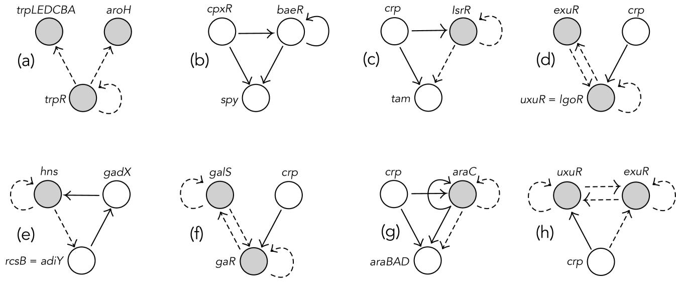
Motifs, small subnetworks that carry out specific functions and occur unusually often, are important building blocks of biological networks. See, for example, [4, 16, 21]. Therefore, the classification of small excitatory-inhibitory networks and their dynamical analysis is a fundamental step in the understanding of the dynamics of biological networks and, consequently, in obtaining answers to important biological questions. Figure 1 illustrates nontrivial 3-node motifs present in real biological networks. More concretely, it shows eight 3-node motifs from the gene regulatory network of Escherichia coli, an organism whose genetic regulatory network, compiled by RegulonDB, has been characterized in considerable detail [7]. For more detail and examples of biological network motifs, see [3].
The importance of biological network motifs, and their dynamics and bifurcations, leads to our interest in formalizing the structure of excitatory-inhibitory (EI) networks and to investigate small examples systematically. This was the motto for our work in [3], where we classify connected 2-node excitatory-inhibitory networks under various conditions.
We work in the coupled cell network formalism of [6, 8, 9, 10, 20], in which nodes (cells) and arrows (connections, directed edges) are partitioned into one or more types. In biological networks it is common to distinguish between two types of connection: excitatory and inhibitory. In standard models these have different dynamic effects. In the coupled cell formalism we represent this distinction by assuming that nodes and arrows have two distinct types. For convenience, we call these ‘excitatory’ and ‘inhibitory’, but the classification is independent of their dynamics.
In the general theory, the dynamics of the network can be prescribed by any system of ordinary differential equations (ODEs) that respects both its topology and the distinction between different types of node or arrow. Such systems of ODEs are said to be admissible for the network. The dynamical interpretation of nodes or arrows as being excitatory (tending to activate the nodes to which they connect) or inhibitory (tending to suppress such activity) is not built into the definition of admissible ODEs, because connections can differ in other ways. See [3, Section 1.3] for remarks on how excitation and inhibition can be defined within the formalism for specific ODE models.
The classification of 2-node excitatory-inhibitory networks in [3] considers different possibilities regarding whether the distinction between the two types of node is maintained, or they are identified, and regarding whether a node can send only one type of output, excitatory or inhibitory, or can have both excitatory and inhibitory outputs. This leads to four different types of excitatory-inhibitory networks: restricted, partially restricted, unrestricted and completely unrestricted. For each type we give in [3] two different classifications. Using results on ODE-equivalence and minimality, we classify the ODE-classes and present a minimal representative for each ODE-class. We also classify all the networks with valence .
In this work, as a continuation of [3], we extend the classification to 3-node excitatory-inhibitory networks. However, here we assume the type of connection is determined by its tail node, as happens for general neuronal networks. In other words, excitatory nodes output excitatory signals and inhibitory nodes output inhibitory signals. This is what we call restricted excitatory-inhibitory (REI) networks in Definition 2.1 below. In Figure 1, networks (a)-(b) have arrows (and nodes) of a single type. Networks (c)-(f) are REI networks. Networks (g)-(h) are not REI networks: some node outputs arrows of both types.
An Example
The 3-node network motif (f) of Figure 1 is an example of an REI network. The black shaded nodes are of one type (say, inhibitory) and the third node is of different type (say, excitatory). Both inhibitory nodes send two inhibitory outputs, which in this network, are directed to the two inhibitory nodes; the excitatory node sends an excitatory signal to one of the inhibitory nodes. In the coupled cell network formalism the main features we retain from this particular network are that it has 3 nodes, two of them are of one type and the third one is of different type. The equal type nodes output arrows of the same type. Different node types output different arrow types. See Figure 2 left. A general admissible system of ODEs consistent with this network has the form
| (1.1) |
where are smooth functions. Each such function captures how the evolution of each node depends on the other nodes. The overbar notation over two variables in the functions and denotes their invariance under permutation of the two variables, which occurs because the corresponding input arrows have the same type. Assuming nodes have internal phase space and node has internal phase space , then , and .
Interpreting the network as a 3-gene Escherichia coli GRN, we may assume that the variable is associated with gene , for . Here, is the concentration of mRNA in gene and is the concentration of protein in gene . We also assume that the time evolution of the cellular concentration of proteins and mRNA molecules is determined by an ODE.(We use this term for a single ODE and for a system.) Moreover, there must be the constraint that a concentration cannot be negative. In this modeling approach, two components of the ODE are associated with each gene . The equation for determines the rate of change of the concentration of the transcribed mRNA; the equation for describes the rate of change of the concentration of its corresponding translated protein. As in [14], a simple example of an admissible system of the form (1.1), where all 3 genes have 2-dimensional node spaces (that is, ), arises by choosing the following functions :
| (1.2) |
Here, as genes are of the same type, we take , and . Also, represent, respectively, degradation of mRNA and protein for gene , and are assumed to be independent of the concentrations of the other molecules in the cell. The function (resp. ) in the equation for gene describes how protein inhibits (resp. activates) mRNA . In this model equation we assume that the effects of the proteins are additive; an alternative typical modeling assumption is that they are multiplicative. See for example [19]. These functions and are generally nonlinear. Typical choices for are the Hill functions:
where is a positive integer. Assuming , since it represents a concentration, converges to as converges to and . This property encodes inhibition into the equations. Assuming the inhibitory edges to be of the same type corresponds to taking . A choice for excitation is the function
where is not necessarily equal to . With the functions as in (1.2), and taking into account the structure of network on the left of Figure 2 (or the 3-gene GRN motif in Figure 1 (f)), equations (1.1) take the form:
| (1.3) |
Thus, for , the rate of change of the concentration of the transcribed mRNA , given by , is the difference between the ‘synthesis term’ ( for and for ), and the ‘degradation term’ . In fact, we can think that the evolution of gene given by is a sum of two parts: one determines the internal dynamics of the gene and the other determines the coupling effect. For , we can consider the internal dynamics to be determined by
and the coupling part by
Alternatively, we can consider the internal dynamics to be determined by
and the coupling part by
This can be interpreted as considering different gene internal dynamics of gene . Similarly, we have two analogous options for the internal dynamics of gene . Taking the second option for the internal dynamics of genes and , we may rewrite (1.2) as
| (1.4) |
In the coupled cell network formalism, the vector field (1.4) determines an admissible coupled cell system for the network on the right of Figure 2, which has the general form
| (1.5) |
where
In the coupled cell network formalism, we say that the two networks of Figure 2 are ODE-equivalent, precisely because every admissible ODE for the network on the right of Figure 2 can be seen as an admissible ODE for the network on the left of Figure 2, and conversely, assuming the node phase spaces of the two networks are the same. Moreover, the network on the right of Figure 2 is the minimal network in terms of number of edges among all 3-node networks that are ODE-equivalent to the networks in Figure 2. See Subsection 2.2 for formal definitions and main results on network admissible ODEs, ODE-equivalence and minimality. In this paper, we use results on network ODE-equivalence and minimality to classify the set of 3-node REI networks into ODE-classes and present minimal representatives for each ODE-class.
Summary of Paper and Main Results
We characterize and classify connected 3-node REI networks. We give a classification under the relation of ODE-equivalence, where two networks are ODE-equivalent if they have the same space of admissible ODEs. Sometimes we consider a restriction on the valence of the nodes. To organize and summarize these results, Table 1 lists the main classifications obtained in this paper, with columns for type of network, bounds on the valence, number of networks in the classification, plus references to associated Figures, Tables and Theorems.
| network | number of | figure | theorem |
|---|---|---|---|
| type | networks | ||
| REI | Figure 5 | Proposition 3.1 | |
| Table 2 | |||
| REI (ODE) | Figure 5 | Proposition 3.2 | |
| REI (ODE) val | 92 | Figure 5 | Proposition 3.3 |
| no auto 2 arrow-types | Table 3 | ||
| REI (ODE) val | 38 | Figure 5 | Proposition 3.3 |
| no auto 1 arrow-type | Table 4 | ||
| REI (ODE) val | 62 | Figure 5 | Proposition 3.3 |
| auto 2 arrow-types | Table 5 | ||
| REI (ODE) val | 35 | Figure 5 | Proposition 3.3 |
| auto 1 arrow-type | Table 6 | ||
| REI val | Figure 6 | Proposition 3.5 | |
| REI val , different conditions | — | Figures 12, 15, 18, 21 | Propositions 3.8, 3.11, 3.14, 3.17 |
Section 2 discusses REI networks from the point of view of the general network formalism of [9, 10, 20]. Subsection 2.1 gives a formal definition of ‘restricted excitatory-inhibitory’ (REI) networks. Subsection 2.2 defines the class of admissible ODEs associated with an REI network. Adjacency matrices are also discussed.
Section 3 characterizes connected 3-node REI networks and classifies them up to ODE-equivalence. Corresponding admissible ODEs are not listed, for reasons of space, but can be deduced algorithmically from the network diagrams. Subsection 3.2 classifies the connected -node REI networks with valence and also classifies their ODE-classes. Subsection 3.3 classifies connected -node REI networks with valence under four different conditions: (i) every node receives one arrow of each type; (ii) only the two excitatory nodes receive one arrow of each type; (iii) only the inhibitory node and one excitatory node receive one arrow of each type; (iv) given any two nodes there is no arrow-type preserving bijection between their input sets.
2. Restricted Excitatory-Inhibitory Networks
In this section we define the class of restricted EI-networks (REI). We assume the networks have two distinct node-types and two different arrow-types , which we may think of as excitatory/inhibitory nodes and excitatory/inhibitory arrows. Moreover, we make the standard simplified modeling assumption that all excitatory arrows are identical and all inhibitory arrows are identical. Without this last assumption, the lists of networks becomes much larger, already for the class of 3-node networks.
In some areas of biology, notably neuroscience, a given node cannot output both an excitatory arrow and an inhibitory one. We make that assumption here. Also, as in [3], we work in the modified network formalism presented in [9], which allows arrows of the same type to have heads of different types. This differs from the formalism of [10, 20], in which arrows of the same type have heads (and tails) of the same type. We remove that condition so that an excitatory (resp. inhibitory) node can send excitatory (resp. inhibitory) arrows to excitatory and/or inhibitory nodes. See [9, Section 9.3] for technical details where it is pointed out that the main network theorems and their proofs remain valid in the more general formalism. See also [3, Remarks 2.1] for a discussion of this approach.
2.1. Formal Definitions
We define restricted excitatory-inhibitory (REI) networks, state our conventions for representing them in diagrams, and give examples.
Definition 2.1.
A network is a restricted excitatory-inhibitory network (REI network) if it satisfies the following four conditions:
(a) There are two distinct node-types, and .
(b) There are two distinct arrow-types, and .
(c) If then .
(d) If then ,
where indicates the tail node of arrow .
Conventions
The following conventions are used throughout the paper without further mention, except as an occasional reminder for clarity.
(a) We represent type nodes by white circles and type nodes by grey circles. Type arrows are solid and type arrows are dashed. (Various other conventions for excitatory/inhibitory arrows are found in the literature; this one is chosen for convenience.)
(b) All classifications are stated up to renumbering of nodes and duality; that is, interchange of ‘excitatory’ and ‘inhibitory’ on nodes and arrows: and .
Example 2.2.
The networks (c)-(f) in Figure 1 are REI networks. However, networks (g)-(h) are not REI networks as some node (the araC gene in network (g) and the crp gene in network (h)) outputs arrows of both types.
Definition 2.3.
(a) In an REI network, every node can receive excitatory and inhibitory arrows: here, the sets of excitatory and inhibitory arrows directed to are denoted by and , and called the excitatory and inhibitory input sets of , respectively. The union is the input set of and the cardinality of is the valence (degree, in-degree) of .
(b)
Two nodes and with the same node-type and valence are said to be input equivalent when and .
We write .
Trivially,
the relation is an equivalence relation, which partitions the set of nodes into
disjoint input classes.
(c)
A network where the nodes are not all input equivalent is inhomogeneous. Otherwise, it is homogeneous.
Remarks 2.4.
(a)
Every REI network is inhomogeneous as by definition it has two distinct node-types, and .
(b) The definition of (robust) synchrony in [9, 10, 20] implies that
synchronous nodes must be input equivalent. Thus for EI networks,
nodes of type cannot synchronize with nodes of type . See also Subsection 2.4.
In this paper we consider connected networks in the sense there is an undirected path between every pair of nodes. We distinguish connected networks according to the existence of a closed directed arrow-path containing every node, or not. In the first case, the network is transitive. Otherwise, it is feedforward.
Example 2.5.
Consider the two networks (e)-(f) in Figure 1. Network (e) is transitive and network (f) is feedforward.
2.2. Admissible ODEs
We adopt the general form of admissible ODEs for a network as defined in [9, 10, 20] with the assumption in this paper that all nodes have the same state space, say for some . Given an EI network with a finite set of nodes, node is represented in the ODE system by the variable which is governed by a system of ordinary differential equations. The word ‘admissible’ is used in the sense that the ODE system encodes information about the node and arrow types. Specifically, when two input equivalent nodes have the same numbers, say , of excitatory arrows and of inhibitory arrows, targeting the two nodes, we specify their dynamics by the same smooth function, say , evaluated at the node and at the corresponding tail nodes of the arrows targeting the node. We follow [3, Definition 2.8]:
Definition 2.6.
A system of ODEs is admissible for an EI network if it has the form
where and the overlines indicate that the function is symmetric in the overlined variables. The node variables are indexed by . The multiset of all tail nodes of input arrows is the union of two subsets: the multiset of all tail nodes of the excitatory input set of node , and the multiset of all tail nodes of the inhibitory input set of node . The functional notation converts these multisets into tuples of the corresponding variables. We use the superscripts and , as a notation convention, to make the distinction between the input variables corresponding to tail nodes in the excitatory and in the inhibitory input sets, respectively. Analogously, when there are two distinct node-types and , we use the superscripts and to make the distinction between the state variable of excitatory and inhibitory nodes.
Moreover, if nodes of the same node-type are in the same input class, that is, there is an arrow-type preserving bijection between the corresponding input sets, then . The evolution of nodes in different input classes is governed by different functions , one for each input class.
Remark 2.7.
Observe that multiple arrows are permitted as there can be distinct excitatory (resp. inhibitory) arrows with the same tail node directed to the same node. Moreover, self-loops are also permitted as a node can input an arrow to itself. In biology, the term autoregulation is used when a node influences its own state.
Example 2.8.
The UNSAT-Feed-Forward-Fiber network in Figure 1 (c), which is one of the 3-node motifs from the gene regulatory network of Escherichia coli, is an REI (inhomogeneous) network. Nodes ‘crp’ and ‘tam’ are type and node ‘IsrR’ is type . We number them as nodes 1, 2 and 3, respectively. There are two type arrows; one from to and the other from to . There are two type arrows; one from to itself and the other from to .
Node has empty input set. Nodes and have excitatory and inhibitory input sets with cardinality . Node is autoregulatory. Thus, although nodes and are of same type, they are not input equivalent, since they have different valences. On the other hand, although nodes and have same excitatory and inhibitory input valences, they are not input equivalent, since they are of different types.
Admissible ODEs are:
| (2.6) |
Here, , where is the node state space, and and are smooth functions.
An -node network can be represented by its adjacency matrix, which is the matrix such that is the number of arrows from node to node . (In the graph-theoretic literature the opposite convention is often used, which gives the transpose of the adjacency matrix defined here.) For an REI network, conditions (c)-(d) of Definition 2.1 allow us to deduce the arrow-types from its adjacency matrix, provided we know the node-types of nodes and . In fact, we consider two node-type matrices, which are both diagonal: given one node-type matrix, the diagonal entry is 1 if node is of that type and zero otherwise. When we need to distinguish the different arrow-types, as is the case in this paper when classifying networks using ODE-equivalence, see Subsection 2.3, we consider arrow-type adjacency matrices, one for each arrow type. For example, for REI-networks, we will consider two arrow-type adjacency matrices, one for excitatory arrows and the other for inhibitory arrows.
Example 2.9.
The adjacency matrix of the UNSAT-Feed-Forward-Fiber network in Figure 1 (c) is
We may also distinguish node- and arrow-types and equip each with its own adjacency matrix. Here there are four:
2.3. ODE-equivalent Networks
As mentioned and exemplified in the Introduction, different networks with the same number of nodes are said to be ODE-equivalent if they have the same set of admissible ODEs, for any choice of node state spaces, when their nodes are identified by a suitable bijection that preserves node state spaces. See [5, 9, 10].
Remarks 2.10.
(a)
A necessary and sufficient condition for two
networks to be ODE-equivalent, using the associated node and arrow adjacency matrices,
is proved in [5, Theorem 7.1, Corollary 7.9].
Specifically, two networks with the same number of nodes are ODE-equivalent if and only if, for a suitable identification of nodes, they have
the same vector spaces of linear admissible maps when node state spaces are .
Equivalently, the adjacency matrices of all node- and arrow-types span the same space.
(b) For REI networks, as mentioned above, the node-types determine the arrow-types,
which implies that the adjacency matrices naturally decompose into four blocks.
The linear condition in (a) preserves this decomposition, so two REI networks are
ODE-equivalent if and only if these components are separately ODE-equivalent.
(c) In fact, using the results in [1, 2] on network minimality, it follows that given an ODE-class of
REI networks, we can distinguish a subclass containing the
REI networks in the ODE-class that have a minimal number of arrows. This is a minimal subclass which
in general need not be a singleton.
Examples 2.11.
(a) The REI network in Figure 3 is ODE-equivalent to the REI
UNSAT-Feed-Forward-Fiber network in Figure 1 (c) and it is minimal.
Moreover, the admissible ODE (2.6) determines an arbitrary dynamical
system in .
(b) The REI network on the right of Figure 2 is ODE-equivalent to the REI 3-gene GRN motif in Figure 1 (f)
and it is minimal.
2.4. Robust Network Synchrony Subspaces
Consider the 3-node REI network on the left of Figure 4. The two excitatory nodes are input equivalent as both receive only one inhibitory arrow. A general admissible ODE-system associated with this network has the form
| (2.7) |
where are smooth functions. We see that any solution of (2.7) with initial condition satisfying say has nodes synchronized for all time, that is,
This property does not depend on the choices of the functions neither the internal node phase spaces . It is determined only by the structure of the network on the left of Figure 4; concretely, the two nodes are of the same node type and each receives one inhibitory arrow from the inhibitory node , which in this example is the unique inhibitory node. Equivalently, we see that the vector field leaves invariant the space , that is,
In this case, we say that is a robust network synchrony space. Restricting (2.7) to , we obtain the system
| (2.8) |
which is admissible for the 2-node network on the right of Figure 4 which is also an REI network. In the terminology of [20], the 2-node network on the right of Figure 4 is the quotient of the network on the left of Figure 4 by the equivalence relation on the node set of the 3-node network with equivalence classes and . This relation is said to be balanced, which is equivalent to the invariance of under the node and arrow adjacency matrices.
These ideas generalize to -node networks and it is proved in [20] that the admissible vector fields for a network leave invariant a linear subspace defined in terms of equalities of certain node coordinates if and only if the equivalence relation on the network node set with classes given by the clusters of nodes whose coordinates are identified is balanced. See [20, Definition 6.4] for the definition of network balanced relation, [9, Proposition 10.20 ] or [10, Section 5], and [20, Theorem 6.5] for the definition of quotient network by a balanced equivalence relation.
For REI networks, it is trivial to show that the restriction of any admissible ODE for an REI network to a robust synchrony subspace is admissible for a smaller network, which is also an REI network. That is, the quotient of an REI network by a balanced equivalence relation on the network node set is also an REI network.
3. Classification of Connected 3-node REI Networks
We now classify REI networks with three nodes, which we assume are connected. Moreover, up to duality and numbering of the nodes, we can assume that the networks have nodes and of type and node of type .
3.1. Connected 3-node REI Networks
In this section we characterize the connected -node REI networks, without imposing any restrictions, and classify them up to ODE-equivalence.
Up to duality any -node REI network is as shown in Figure 5, for a suitable choice of nonnegative integer arrow multiplicities , , , , , where , .
The adjacency matrices are
Proposition 3.1.
Proof.
A -node REI network is connected if and only if the union of the input and output sets of each node, excluding self-coupling arrows, is nonempty. That is, if and only if at least one multiplicity is nonzero in each of the sets
The possible combinations are listed in Table 2. ∎
Proposition 3.2.
The -node REI networks are those in Figure 5, for a suitable choice of nonnegative integer arrow multiplicities , , , , , where , .
Up to ODE-equivalence and minimality, we can assume that is zero and at least one of or is zero.
-
Moreover, either
-
and are coprime, if both nonzero, or
-
and , or and , or
-
.
-
-
If , then
-
the nonzero , , are coprime, or
-
, if , , , or
-
, .
-
-
If and , then
-
and the nonzero , , are coprime, or
-
, .
-
Proof.
Up to ODE-equivalence, we can assume that , so
Thus, if , we can set , and vice versa. If both and are nonzero, we can assume they are coprime.
Moreover, up to ODE-equivalence, we can assume that, at least one, of or is zero. If and we can assume that and the nonzero , for , are coprime.
If both and are zero then
then we can assume that the nonzero , for , are coprime. ∎
3.2. Connected 3-node REI Networks with Valence
In this section we classify the connected -node REI networks with valence . We start by classifying them up to ODE-equivalence.
| nonzero multiplicities | ODE-classes |
|---|---|
| 4 | |
| 2 | |
| 4 | |
| 2 | |
| 2 | |
| 1 | |
| 2 | |
| 1 | |
| 2 | |
| 3 | |
| 4 | |
| 2 | |
| 1 | |
| 2 | |
| 2 | |
| 2 | |
| 4 | |
| 3 | |
| 1 | |
| 3 | |
| 1 | |
| 1 | |
| 3 | |
| 4 | |
| 2 | |
| 4 | |
| 3 | |
| 4 | |
| 2 | |
| 1 | |
| 2 | |
| 1 | |
| 2 | |
| 4 | |
| 3 | |
| 1 | |
| 2 | |
| 1 | |
| 1 | |
| 3 |
Proposition 3.3.
Any connected -node REI network with valence is ODE-equivalent to the network in Figure 5, where, under minimality, and
Proof.
| nonzero multiplicities | ODE-classes |
|---|---|
| 3 | |
| 7 | |
| 2 | |
| 4 | |
| 7 | |
| 3 | |
| 3 | |
| 2 | |
| 3 | |
| 1 | |
| 3 |
Lemma 3.4.
If is a connected -node REI network with input valence , where nodes are of type and node is of type , then the subnetwork of containing nodes and all arrows between these two nodes is a -node REI network with input valence .
Proof.
The subnetwork of containing nodes is a -node network where node is of type and node is of type . Since is REI then node outputs only excitatory arrows and node outputs only inhibitory arrows. Therefore is also an REI network. ∎
| nonzero multiplicities | ODE-classes |
|---|---|
| 2 | |
| 1 | |
| 2 | |
| 2 | |
| 2 | |
| 4 | |
| 2 | |
| 4 | |
| 1 | |
| 2 | |
| 1 | |
| 2 | |
| 2 | |
| 3 | |
| 4 | |
| 2 | |
| 4 | |
| 2 | |
| 4 | |
| 2 | |
| 1 | |
| 2 | |
| 2 | |
| 1 | |
| 2 | |
| 4 | |
| 2 |
| nonzero multiplicities | ODE-classes |
|---|---|
| 7 | |
| 4 | |
| 4 | |
| 2 | |
| 4 | |
| 7 | |
| 2 | |
| 1 | |
| 2 | |
| 2 |
Proposition 3.5.
The set of connected -node REI networks with valence comprises the networks in Figure 6.
Proof.
We enumerate the set of connected -node REI networks with valence using Lemma 3.4. We can assume that nodes and have type and node has type .
Consider the subnetwork of containing node (of type ) and node (of type ) and all arrows between these nodes. This is a -node REI network with valence . If is connected then it is one of the networks in Figure 7 (Figure 7 in [3]), where node is of type and node is of type . If is not connected then is one of the networks in Figure 8. The options for arrows from to node and from node to are shown in Figure 9.
3.3. Connected 3-node REI Networks with Valence 2
In this section we classify connected -node REI networks with valence . We consider four different cases:
-
(i)
Every node receives one arrow of each type;
-
(ii)
Only the two excitatory nodes receive one arrow of each type;
-
(iii)
Only the inhibitory node and one excitatory node receive one arrow of each type;
-
(iv)
Given any two nodes there is no arrow-type preserving bijection between their input sets.
We start by classifying the -node REI networks of valence that are almost homogeneous; that is, where every node receives exactly one excitatory and one inhibitory arrow. (The obstacle to exact homogeneity is that the nodes have different types.)
Lemma 3.6.
If is an almost homogeneous connected -node REI network of valence , with and and arrow-types and , then the subnetwork of containing only arrows of type is the network in Figure 10.
Proof.
Since is an almost homogeneous REI and node is the only one of type , every node receives one arrow of type from node . ∎
Lemma 3.7.
If is an almost homogeneous connected -node REI network of valence , with and , and arrow-types and , then the subnetwork of containing only arrows of type is one of the networks in Figure 11.
Proof.
Since is an almost homogeneous REI and node is the only of type , every node receives one arrow of type from nodes or . ∎
Proposition 3.8.
Any almost homogeneous connected -node REI network of valence with , , and two arrow-types and , is one of the networks in Figure 12. These are not ODE-equivalent. Each of these networks has a unique -dimensional robust synchrony subspace where only nodes are synchronized; see Remark 2.4(b) and Subsection 2.4.
Proof.
We can assume that REI networks have nodes and of type and node of type . If is an almost homogeneous connected -node REI network with valence then the subnetwork containing only the arrow-type is the network in Figure 10, see Lemma 3.6, and the subnetwork of containing only arrow-type is one of the networks listed in Figure 11, see Lemma 3.7. The subnetwork containing only arrow-type is symmetric under transposition of nodes and . We obtain the networks in Figure 12. ∎
We consider now 3-node REI networks of valence 2 which are inhomogeneous, where nodes are input equivalent, each receives one arrow of each type, but node does not receive one arrow of each type.
Lemma 3.9.
Let be a connected -node REI network of valence , with , , and arrow-types and . Assume that nodes and are input equivalent, receiving one arrow of each type. Then the subnetwork of containing only the arrow-type is the network in Figure 13.
Proof.
Since nodes of are input equivalent and is REI, node is the only one of type , and nodes receive one arrow of type from node . ∎
Lemma 3.10.
Let be a connected -node REI network of valence with , , and arrow-types and . Assume that nodes and are input equivalent, each receiving one arrow of each type. Then the subnetwork of containing only the arrow-type is one of the networks in Figure 14.
Proof.
Since is REI and nodes and are of type , each of nodes receives one arrow of type from nodes or . ∎
Proposition 3.11.
Any connected -node REI network of valence , where the two excitatory nodes are input equivalent receiving one arrow of each type and the inhibitory node does not receive one arrow of each type, is one of the networks in Figure 15. All these networks have exactly one -dimensional robust synchrony subspace where nodes and are synchronized.
| (NH.1) | (NH.2) | (NH.3) |
Proof.
We can assume that the REI network has nodes and of type and node of type . Suppose that is a minimal connected -node REI network with valence , input equivalence relation , and where nodes and receive one arrow of each type. Then the subnetwork containing only arrow-type is the network in Figure 13, see Lemma 3.9, and the subnetwork of containing only arrow-type is one of the networks in Figure 14, see Lemma 3.10. The subnetwork containing only arrow-type is symmetric under transposition of nodes and . We obtain the networks in Figure 15. Clearly the only possible robust synchrony subspace must have nodes 1 and 2 synchronized. ∎
We consider 3-node REI networks of valence 2, where we assume now that all three nodes are not input equivalent, but nodes receive one arrow of each type.
Lemma 3.12.
Let be a connected -node REI network of valence with , , and arrow-types and . Assume that and that nodes and receive one arrow of each type. Then the subnetwork of containing only arrow-type is the network in Figure 16.
Proof.
Since nodes of receive both an arrow of type and is REI, node is the only one of type , and nodes receive one arrow of type from node . ∎
Recall from Definition 2.3 that denotes input equivalence. We now prove:
Lemma 3.13.
Let be a connected -node REI network of valence , with , , and arrow-types and . Assume that and that nodes and receive one arrow of each type. Then the subnetwork of containing only arrow-type is one of the networks in Figure 17.
Proof.
Since is REI and nodes and are those of type , every node receives one arrow of type from node or . ∎
Proposition 3.14.
Any connected -node REI network of valence , where two nodes are excitatory, one node is inhibitory, and all three nodes are not input equivalent but where one excitatory node and the inhibitory node receive one arrow of each type, is one of the networks listed in Figure 18.
| (NH.4) | (NH.5) | (NH.6) | (NH.7) |
|---|---|---|---|
| (NH.8) | (NH.9) | (NH.10) | (NH.11) |
Proof.
We can assume that nodes and have type and node has type . Let be a connected -node REI network with valence , and input equivalence relation , where nodes and receive one arrow of each type. Then the subnetwork containing only arrow-type is the network in Figure 16, see Lemma 3.12 and the subnetwork of containing only arrow-type is one of the networks listed in Figure 17, see Lemma 3.13. We obtain the networks in Figure 18. ∎
We consider 3-node REI networks of valence 2, where we now assume that, given any two nodes, there is no arrow-type preserving bijection between their input sets:
| (3.9) |
Thus, each node lies in a different input equivalence class, that is, .
Lemma 3.15.
Proof.
The network is REI and node is the only one of type . By (3.9), only two nodes receive arrows of type from node . Moreover, one receives one arrow and the other two arrows. ∎
Lemma 3.16.
Proof.
The network is REI and nodes and are those of type . By (3.9) only two nodes receive arrows of type from nodes and . Moreover, one receives one arrow and the other receives two arrows. ∎
Proposition 3.17.
Proof.
Up to duality, REI networks have nodes and of type and node of type . If is a connected -node REI network with valence , input equivalence relation and satisfying (3.9), then the subnetwork containing only arrow-type is one of the networks listed in Lemma 3.15, and the subnetwork of containing only arrow type is one of the networks listed in Lemma 3.16. We obtain the networks in Figure 21. ∎
4. Conclusions
Motivated by the growing interest in network motifs and their functionality in biological networks, and following the work in [3], we give a characterization of the connected 3-node restricted excitatory-inhibitory networks. Our classifications are up to renumbering of the nodes and duality – switch nodes and arrows types from ‘excitatory’ to ’inhibitory’, and vice versa. Although there is an infinity of connected 3-node restricted excitatory-inhibitory networks, when we restrict to networks with valence less or equal to – each node receives at most inputs – we get a finite number. Taking our characterization further, we also list those networks with valence exactly equal to 2, under different conditions on the input arrows of the 3 nodes, ranging from all nodes receiving an arrow of each type to all having non-isomorphic input sets. Both, for all connected 3-node restricted excitatory-inhibitory networks and those with valence less or equal to , we give their characterization under ODE-equivalence. Moreover, we give a minimal representative for each ODE-class.
The next step for future work in our systematic study is to explore the dynamics, in particular the bifurcations, of these 3-node restricted excitatory-inhibitory motifs. This will be in line to what is done in [14] for six particular motifs that occur as functional building blocks in gene regulatory networks, where the state of each gene is modeled in terms of two variables: mRNA and protein concentration. The study in [14] explores the patterns of synchrony (fibration symmetries) of the motifs and considers both all possible network admissible models as well as special specializations to simple models based on Hill functions and linear degradation.
Acknowledgments
MA and AD were partially supported by CMUP, member of LASI, which is financed by national funds through FCT – Fundação para a Ciência e a Tecnologia, I.P., under the projects with reference UIDB/00144/2020 and UIDP/00144/2020.
References
- [1] M.A.D. Aguiar and A.P.S. Dias. Minimal coupled cell networks, Nonlinearity 20 (2007) 193–219; doi:10.1088/0951-7715/20/1/012.
- [2] M.A.D. Aguiar and A.P.S. Dias. Coupled cell networks: minimality, Proc. Appl. Math. Mech. 7 (2007) 1030501–1030502; doi:10.1002/pamm.200700991.
- [3] M. Aguiar, A. Dias, and I. Stewart. Classification of 2-node excitatory-inhibitory networks, Mathematical Biosciences 373 (2024) 109205; doi: 10.1016/j.mbs.2024.109205.
- [4] E. Borriello. The local topology of dynamical network models for biology, Journal of Complex Networks, 12 (2) (2024) cnae007; https://doi.org/10.1093/comnet/cnae007.
- [5] A.P.S. Dias and I. Stewart. Linear Equivalence and ODE-equivalence for coupled cell networks, Nonlinearity 18 (2005) 1003–1020; doi:10.1088/0951-7715/18/3/004
- [6] M. Field. Combinatorial dynamics, Dynamical Systems 19 (2004) 217–243; doi:10.1080/14689360410001729379.
- [7] S. Gama-Castro et al. RegulonDB version 9.0: high-level integration of gene regulation, coexpression, motif clustering and beyond, Nucleic Acids Res. 44 (2016) D133-D143.
- [8] M. Golubitsky and I. Stewart. Nonlinear dynamics of networks: the groupoid formalism, Bull. Amer. Math. Soc. 43 (2006) (3) 305–364; doi:10.1090/S0273-0979-06-01108-6.
- [9] M. Golubitsky and I. Stewart. Dynamics and Bifurcation in Networks: Theory and Applications of Coupled Differential Equations, SIAM, Philadelphia 2023; doi:10.1137/1.9781611977332.
- [10] M. Golubitsky, I. Stewart, and A. Török. Patterns of synchrony in coupled cell networks with multiple arrows, SIAM J. Appl. Dyn. Sys. 4 (2005) 78–100; doi:10.1137/0406126.
- [11] C.L. Grove and R.P. Gunsalus. Regulation of the aroH operon of Escherichia coli by the tryptophan repressor, J Bacteriol. 169 (1987) 21582164.
- [12] I. Leifer, F. Morone, S.D.S. Reis, J.S. Andrade Jr., M. Sigman, and H.A. Makse. Circuits with broken fibration symmetries perform core logic computations in biological networks, PLOS Computational Biology (2020); doi:10.1371/journal.pcbi.1007776 0.
- [13] H.A. Makse, Genetic circuits, preprint 2020.
- [14] H.A. Makse, S.D.S. Reis, and I. Stewart. Dynamics and bifurcations in genetic circuits with fibration symmetries, J. R. Soc. Interface, to appear.
- [15] H.A. Makse, I. Stewart, P. Boldi, and F. Sorrentino. Symmetries of Living Systems: Graph Fibrations and Cluster Synchronization in Biological Networks, Cambridge University Press, to appear.
- [16] R. Milo, S. Shen-Orr, S. Itzkovitz, N. Kashtan, D. Chklovskii, and U. Alon. Network motifs: simple building blocks of complex networks, Science 298 (2002) 824–827; doi:10.1126/science.298.5594.824.
- [17] F. Morone, I. Leifer, and H.A. Makse. Fibration symmetries uncover the building blocks of biological networks, Proc. Nat. Acad. Sci. USA 117 (2020) 8306–8314; doi:10.1073/pnas.191462811.
- [18] F. Morone, and H.A. Makse. Network symmetries of living systems, preprint.
- [19] A. Polynikis, S.J. Hogan and M. di Bernardo. Comparing different ODE modelling approaches for gene regulatory networks, Journal of Theoretical Biology, 261 (2009) (4) 511–530; doi:10.1016/j.jtbi.2009.07.040.
- [20] I. Stewart, M. Golubitsky and M. Pivato. Symmetry groupoids and patterns of synchrony in coupled cell networks, SIAM J. Appl. Dynam. Sys. 2 (2003) 609–646; doi:10.1137/S1111111103419896.
- [21] J.J. Tyson and B. Novák. Functional motifs in biochemical reaction networks, Ann. Rev. Phys. Chem. 61 (2010) 219–240; doi:10.1146/annurev.physchem.012809.103457.