Cloud-by-cloud, multiphase, Bayesian modeling: Application to four weak, low ionization absorbers
Abstract
We present a new method aimed at improving the efficiency of component by component ionization modeling of intervening quasar absorption line systems. We carry out cloud-by-cloud, multiphase modeling making use of cloudy and Bayesian methods to extract physical properties from an ensemble of absorption profiles. Here, as a demonstration of method, we focus on four weak, low ionization absorbers at low redshift, because they are multi-phase but relatively simple to constrain. We place errors on the inferred metallicities and ionization parameters for individual clouds, and show that the values differ from component to component across the absorption profile. Our method requires user input on the number of phases and relies on an optimized transition for each phase, one observed with high resolution and signal-to-noise. The measured Doppler parameter of the optimized transition provides a constraint on the Doppler parameter of H i, thus providing leverage in metallicity measurements even when hydrogen lines are saturated. We present several tests of our methodology, demonstrating that we can recover the input parameters from simulated profiles. We also consider how our model results are affected by which radiative transitions are covered by observations (for example how many H i transitions) and by uncertainties in the parameters of optimized transitions. We discuss the successes and limitations of the method, and consider its potential for large statistical studies. This improved methodology will help to establish direct connections between the diverse properties derived from characterizing the absorbers and the multiple physical processes at play in the circumgalactic medium.
keywords:
galaxies: active : quasars: absorption lines – quasars: general1 INTRODUCTION
The circumgalactic medium (CGM) is the tenuous, multiphase medium in the environment of a galaxy. It plays an important role in steering the evolution of galaxies. The massive reservoir of gas in the CGM seeds the formation of stars which evolve and distribute their energy and content back into the galaxy. CGM gas of galaxies can be probed in intricate detail by using metal absorption lines (e.g., Bergeron 1986; Bergeron & Boissé 1991; Lanzetta & Bowen 1992; Steidel & Sargent 1992; Churchill et al. 1996, 2000; Churchill et al. 2020; Adelberger et al. 2005; Kacprzak et al. 2008, 2015, 2019; Chen & Mulchaey 2009; Steidel et al. 2010; Nielsen et al. 2013a, b; Stocke et al. 2013; Werk et al. 2013; Bordoloi et al. 2014; Turner et al. 2014; Johnson et al. 2015; Richter et al. 2016; Keeney et al. 2017; Muzahid et al. 2018) observed in the spectra of background quasars. Absorption-line spectroscopic studies provide information about the metallicities, densities, temperatures, and kinematic structure of various parcels of gas along the lines of sight. These studies are important because they potentially allow us to learn about the processes that supply inflowing gas to the galaxy, enrich the surroundings with metal-rich outflows, minor and major mergers, and send enriched gas back to the galaxy as recycled accretion.
In this paper, we present a new Bayesian method for extracting the physical properties of the multiphase gaseous medium probed by quasar absorption-line systems. To demonstrate the method, we apply it to four, well-studied, weak, low ionization, systems, also known as weak Mg ii absorbers (Narayanan et al. 2005). These systems were chosen because they are relatively simple in the number of low ionization components, but still have multi-phase structure, and also because the origins of these tiny pockets of high metallicity, far from galaxy centers, are of particular interest.
Weak Mg ii-absorbers are defined by rest frame equivalent width 0.3 Å. Unlike strong Mg ii absorbers, which are typically found within kpc of a luminous galaxy (Nielsen et al. 2013b, 2018), the weak Mg ii absorbers are found to be associated with lower neutral hydrogen column densities, and are at larger impact parameters within the circumgalactic environment, typically kpc (Nielsen et al. 2013b, 2018). Churchill et al. (1999) conducted the first systematic survey of weak Mg ii absorbers in the redshift range using HIRES/Keck spectra, and found that the number of weak absorbers per unit redshift of is 4 times higher than that of the Lyman limit systems (LLSs) which have neutral hydrogen column density cm-2, indicating an origin of the weak absorbers in sub-LLSs (Churchill et al. 2000). A tantalizing aspect of the weak Mg ii-absorbers is that, generally, their low ionization phases exhibit near-solar to super-solar metallicities (Rigby et al. 2002; Lynch & Charlton 2007; Misawa et al. 2008; Narayanan et al. 2008) in spite of the fact that luminous galaxies are typically 50200 kpc away. Detailed photoionization models of the intermediate redshift, weak Mg ii-absorbers show that they often have two phases, a high-density region/s that is 1-300 pc thick and produces narrow (a few km s-1) low-ionization lines, and kiloparsec-scale, lower density region/s that produces broader, high-ionization lines (Charlton et al. 2003; Narayanan et al. 2007). By comparing the relative number of Mg ii and C iv absorbers, Milutinović et al. (2006) concluded that the low ionization absorption must occur in flattened or filamentary structures that occupy more than half the solid angle subtended by structures that produce only C iv absorption.
Studies of weak absorbers at low- offer the advantage of ease of detection of host galaxies. At low redshift, , Narayanan et al. (2005) measured for weak Mg ii absorbers (with Å) using Si ii and C ii as proxies in /COS spectra. This is smaller than expected based on the evolution expected for the intermediate redshift population, given the decreasing extragalactic background radiation. This is because the low redshift population should consist both of 1-300 pc absorbers that gave rise to Mg ii absorption at intermediate redshift, and larger clouds that gave rise only to higher ionization (C iv) absorption at intermediate redshift. Understanding which of these types of absorbers dominate the population at low redshift is important to understanding the processes that produce these mysterious, high metallicity objects abundant in the CGM.
More generally, both observational and theoretical studies (e.g., Stinson et al. 2012; Ford et al. 2013; Shen et al. 2013; Suresh et al. 2016) of absorbers reveal the existence of cool (104 K) and warm-hot (105-106 K) phases in the CGM, often all detected along the same sightline to the background quasar. Different ionization states of material trace different phases of gas, which have different densities and temperatures. Cooler, higher-density gas is traced by lower-ionization species (e.g., Mg ii, Si ii) and shows structure on smaller scales compared to the warmer and/or lower-density phase (e.g., C iv or O vi). Length scales of the lower ionization clouds range from 1 pc (McCourt et al. 2012; Liang & Remming 2020) to a few kpc. As mentioned above, strong Mg ii absorption is detected along most sightlines within an impact parameter of 50 kpc from a galaxy (Nielsen et al. 2013a), while weaker Mg ii absorption is found at a median impact parameter of 166 kpc (Muzahid et al. 2018). C iv is often seen out to 100 kpc (Chen et al. 2001; Bordoloi et al. 2014), while O vi is seen out to at least 150 kpc (Prochaska et al. 2011; Tumlinson et al. 2011; Stocke et al. 2013; Liang & Chen 2014; Pointon et al. 2019) of star forming galaxies, but not around quiescent galaxies. Gas traced by H i absorption is seen well beyond (Liang & Chen 2014; Borthakur et al. 2015).
Interpretation of the rich absorption line data is aided by identification of galaxies near the quasar sightlines. It is expected that the orientations of the galaxies will correlate with absorption properties (Bordoloi et al. 2011; Bouché et al. 2012; Kacprzak et al. 2012; Kacprzak et al. 2015; Nielsen et al. 2015). In the simplest view, galactic winds due to episodes of star formation are expected to produce high metallicities in the outflowing gas, and should be seen primarily along the minor axis (Muzahid et al. 2015; Nielsen et al. 2015; Pointon et al. 2019; Schroetter et al. 2019; Peroux et al. 2020). Inflowing pristine gas from the intergalactic medium would be expected to flow in along the major axis. Another important observational result is a bimodality in the metallicity of partial Lyman limit systems, with the high metallicity peak at = and the low metallicity peak at = (Lehner et al. 2013). It has been hypothesized that this bimodality could be due to the contrast between outflowing and infalling material.
A coherent and logical picture is beginning to emerge from the data (Tumlinson et al. 2017), however, there are some significant problems plaguing interpretations, and the root cause of these problems could be the methods used to derive the properties of the gas from the absorption profiles, particularly the metallicities. Often the total column density (integrating over all components at all velocities) of a given metal line transition is compared to the total column density of hydrogen, in the context of photoionization models, to derive the metallicity. This overlooks the importance of phase structure, with more than one phase contributing to absorption at a single velocity i.e. some transitions could have contributions from two different phases which can lead to an inaccurate estimate of ionization parameter, and thus a systematic error in deriving a single metallicity value. In other words, the average parameters inferred for a system may “wash out” contributions from regions of gas that have metallicities and densities that differ significantly from the means, and the possibility of conditions that significantly change with velocity because of changes in physical conditions along the line of sight. Simulations (Churchill et al. 2015; Peeples et al. 2019) indicate absorption arises in lots of places along the sightline, motivating why multiple metallicities are expected.
In a recent study, Zahedy et al. (2019) have carried out a systematic analysis of 16 intermediate-redshift (=0.21-0.55) luminous red galaxies (LRGs), finding metal-poor absorbing components with 1/10 solar metallicity in half of the LRG haloes in tandem with solar and super-solar metallicity gas in the same halo, suggestive of poor chemical mixing and complex multiphase structure in these haloes. This highlights the importance of resolving multiple components of an absorption system using high resolution absorption spectra, which otherwise is missed by ionization studies that make use of only the integrated H i and metal column densities along individual sightlines.
This work improves the efficiency of component by component modeling that has been successful in recovering the physical conditions for various individual absorbers (e.g. Churchill & Charlton 1999; Charlton et al. 2000; Ding et al. 2003a; Charlton et al. 2003; Ding et al. 2003b; Zonak et al. 2004; Ding et al. 2005; Masiero et al. 2005; Lynch & Charlton 2007; Misawa et al. 2008; Lacki & Charlton 2010; Jones et al. 2010; Muzahid et al. 2015; Richter et al. 2018; Rosenwasser et al. 2018). Rather than averaging over components and phases, it is possible to determine how much of the H i is associated with these different phases in order to derive separate metallicities for various clouds. Resolving the individual clouds allows us to break the degeneracy for components on the flat part of the Ly curve of growth, even with coverage of just saturated H i lines, and derive metallicity constraints for different parcels of gas along the line of sight. It is important to do so because different processes e.g., outflows (Bouché et al. 2012; Bordoloi et al. 2014; Rubin et al. 2014; Schroetter et al. 2016), pristine accretion (Rubin et al. 2012; Martin et al. 2012; Danovich et al. 2015), recycled accretion (Ford et al. 2014), minor and major mergers (Martin et al. 2012; Anglés-Alcázar et al. 2017), are surely contributing to the same system, and it is expected that conditions will vary significantly along a line of sight which can span hundreds of kpc spatially (Churchill et al. 2015; Peeples et al. 2019). This will lead to a more meaningful comparison to galaxy properties. For example, Pointon et al. (2019) did not find a difference between the metallicities of absorbers found within an impact parameter of 200 kpc along the major and the minor axes of isolated galaxies. Based on cosmological hydrodynamic simulations, a larger metallicity is expected along the minor axis due to outflows and a lower metallicity along the major axis due to inflows (Peroux et al. 2020). However, an observational trend could exist, for example, for the minor axis to have some, but not all, high metallicity components, or for the minor axis to have one or more low metallicity components. Such results would be “washed out” by deriving an average metallicity for all gas along a line of sight, which clearly often has multiple complex origins. For some datasets/projects the new analysis could be transformative, however to make it feasible to use for large statistical studies it is important that the analysis is semi-automated and robust.
In this paper, we describe a new method to derive the physical properties of quasar absorption line systems using the photoionization code cloudy (ver 17.01; Ferland et al. 2017), Bayesian methods, and parallel processing to efficiently obtain results. Though the code requires some human intervention to choose transitions that define the phase structure, it is mostly automated, and provides uncertainties on parameters in the context of the assumed structure. The paper is organized as follows: in Section 2 we describe the spectral observations that are analysed in this work; in Section 3 we describe the methodology used to determine the physical conditions of an absorber; in Section 4 we present the results and discuss our findings, comparing to previous work, applying tests, and discussing possible limitations. We conclude in Section 5 by discussing the limitations and potential of our cloud-by-cloud, multiphase, Bayesian modeling (CMBM) method. Throughout this work, we assume a cosmology with km s-1 Mpc-1, , and Abundances of heavy elements are given in the notation with solar relative abundances taken from Grevesse et al. (2010). All the distances given are in physical units. All the logarithmic values are presented in base-10.
2 OBSERVATIONS
| QSO. | RA | Dec | Instrument | PIDc | Observed | Observation | ||
| (J2000) | (J2000) | Wavelength (Å) | Date | |||||
| HE0153-4520 | 28.80500 | 0.451 | 0.22596 | COS | 11541 | 1135-1794 | 2002-12-19 | |
| UVES | 293.A-5038(A) | 3045-6650 | 2014-10-26 | |||||
| PG1116+215 | 169.78583 | 21.32167 | 0.176 | 0.13849 | FUSE | P101 | 979-1189 | 2001-04-22 |
| COS | 12038 | 1136-1794 | 2011-10-25 | |||||
| STIS (E140M) | O5E702010 | 1155-1602 | 2000-06-30 | |||||
| STIS (E230M) | O5A302030 | 2010-2817 | 2000-05-15 | |||||
| HIRES | U152Hb | 3104-5901 | 2006-06-02 | |||||
| PHL1811 | 328.75623 | -9.37361 | 0.190 | 0.07776, 0.08094 | FUSE | P108 | 979-1189 | 2003-06-02 |
| COS | 12038 | 1135-1794 | 2010-10-29 | |||||
| STIS (G230MB) | O6CT46010 | 2758-2910 | 2001-10-22 | |||||
| HIRES | U149Hr | 3101-5897 | 2007-09-17 |
Notes– a QSO redshift from NED; b Absorber redshift; c proposal ID.
We apply our methods to four low redshift absorption line systems from the COS-Weak sample (Muzahid et al. 2018). The background quasars in this study have UV spectra from the Cosmic Origins Spectrograph (COS) instrument on the Hubble Space Telescope () and optical spectra from High Resolution Echelle Spectrometer (HIRES) installed on the Keck telescope or Ultraviolet and Visual Echelle Spectrograph (UVES) installed on the Very Large Telescope (VLT). The four absorption systems that we consider have spectroscopic redshifts . These weak, low-ionization systems are relatively simple ones compared to some stronger low-ionization absorbers, but they are expected to have multiple gas phases and provide good test cases for our methodology. Table 1 presents the details of the observations of the four systems studied in this work.
2.1 COS, FUSE and STIS Spectra
The UV spectra in the COS-Weak sample are taken from the archive of /COS observations using the G130M and G160M gratings spanning observed wavelength ranges 1135-1457 Å and 1399-1794 Å, respectively. The spectra have an average resolving power of and cover a range of ions including the H i Lyman series, C ii, C iii, C iv, N v, O vi, Si ii, Si iii and Si iv. The /COS spectra were obtained from the archive already reduced using the calcos pipeline software (Massa et al. 2013), with individual exposures aligned and co-added, weighted by their exposure times. The spectra are rebinned to the Nyquist sampling rate. FUSE spectra for three absorbers in our sample were available. The observations were obtained already processed with the calfuse pipeline (ver. 3.2.3). Zero point offset correction was carried out on this pre-processed data using the approach described in Wakker (2006). The spectra have an average resolving power of . STIS spectra for three absorbers in our sample were available. We make use of COS data when STIS and COS both have coverage of a transition of interest because the COS spectra have significantly higher signal-to-noise, , ratio compared to the STIS data. When a transition is not covered by COS, we make use of STIS observations.
We perform continuum normalization of the data by fitting a cubic spline to the spectrum. We estimated the uncertainties in the continuum fits using “flux randomization” Monte Carlo simulations (e.g. Peterson et al. 1998), varying the flux in each pixel of the spectrum by a random Gaussian deviate based on the spectral uncertainty. The pixel-error weighted average and standard deviation of 1000 iterations was adopted as the flux and uncertainty of the continuum fit, respectively.
2.2 Ground-based Optical Quasar Spectra
When available, we use higher resolution optical spectra to complement the UV spectra because transitions including Mg i, Mg ii, Fe ii, and Ca ii are especially useful in revealing the presence of multiple components for absorption systems at redshifts of . The spectra have an average resolving power of . The HIRES spectra were reduced using the Mauna Kea Echelle Extraction (MAKEE) package. The UVES spectra were reduced using the European Southern Observatory (ESO) pipeline (Dekker et al. 2000) and the UVES Post-Pipeline Echelle Reduction (UVES POPLER) code (Murphy 2016; Murphy et al. 2019). The program numbers and dates of these observations are also listed in Table 1.
3 METHODOLOGY
We model the observed absorption system using the photoionization code cloudy, and synthesize the expected absorption profiles and compare them to the observed profiles in order to infer the physical conditions of the absorbing gas. What makes this method different from other researchers’ methods is that we model the entire absorption system across all transitions by splitting it into its constituent clouds.
We begin by choosing a “trustworthy” low ionization species (the “optimized ion”) for a Voigt profile (VP) fit, meaning one with lines that are unsaturated, and observed at a high resolution, and with a large . The starting point is a fit of Voigt profiles to all transitions within this single ionization species (each parcel of gas described by a single VP will be called a “cloud”). For this optimized transition we determine the parameters of column density (), Doppler parameter (), and redshift () for each cloud using a Monte Carlo technique employed using PyMultiNest (Buchner et al. 2014). PyMultiNest is a python implementation of MultiNest (Feroz et al. 2009), which is a robust nested sampling method that draws a new, uniformly random point with higher likelihood through an ellipsoidal rejection sampling scheme (Shaw et al. 2007). It is efficient at sampling from a multimodal posterior distribution. We model Voigt profiles using an analytic approximation (Tepper-García 2006) for the Voigt-Hjerting function as implemented in the VoigtFit package (Krogager 2018). We obtain VP fits to the absorption profiles for the optimized ion, allowing for more than one component. We fit the profiles of the optimized ion with a VP model corresponding to the highest log-evidence and the least model complexity. After we determine the observed values of , , and for each cloud, we use the parameters of that VP fit for the optimized ion as a starting point for models in cloudy.
cloudy has many parameters that can be adjusted. The two most important parameters are metallicity relative to solar abundance () and ionization parameter (), defined by , where is the volume density of ionizing photons. Ionization parameter serves as a direct proxy for the hydrogen number density, but may be more intuitive when thinking of contributions of different clouds to the observed ionization states. We adopt the Haardt & Madau (2012)[HM12] model for the extragalactic background radiation (EBR) to determine at the given redshift. The systematic effects arising from the choice of the EBR are discussed in Keeney et al. (2017). We adopt the HM12 model as it best reproduces the low-redshift H i column density distribution (Danforth et al. 2016) for 14 (Shull 2014). We assume a solar abundance pattern (Grevesse et al. 2010) for our modeling. Detailed constraints on abundance pattern are not possible without higher coverage of a larger number of transitions.
It is a time-consuming endeavor to construct cloudy models component-by-component and phase-by-phase for individual absorbers because of the limitations imposed by serial computing. However, it is clear that doing so will lead to a significant gain in our ability to correctly infer the presence of metallicity structure in the CGM. To increase efficiencies we have developed robust python based codes that employ distributed parallel processing on the CyberLAMP infrastructure 111https://wikispaces.psu.edu/display/CyberLAMP to obtain models in a shorter time.
The cloudy photoionization equilibrium (PIE) models are generated for the identified optimized ion tracing the low ionization gas phase for a broad range of values over the grid in the range: [-3.0,1.5] and [-6.0, 0.0], obtained with a step-size of 0.1. The cloudy models are then linearly interpolated onto the grid with a spacing of 0.01 dex. The interpolating function is generated by triangulating the input data with Qhull (Barber et al. 1996), and on each triangle performing linear barycentric interpolation. The interpolation error is of the order , being 0.1, and introduces only small errors 0.01 dex in and . The total column density of hydrogen, , is adjusted for each model until the column density of the optimized ion is matched for each point on the grid. We allow for an uncertainty of 0.05 dex in the column density matching when generating the cloudy models. The uncertainties arising due to the interpolation error and the error in column density are not accounted for in our error estimation, but are usually negligible in comparison to other sources of error. We quote 2 uncertainties in our results for the best model parameter values, which account only for the photon noise in the comparison between the synthesized model profiles and the observed spectra.
We then determine the parameters that best describe the conditions (, ) present in each one of the absorbers again using PyMultiNest. The posterior distribution of the parameters, which is proportional to the product of priors and likelihood, is determined by using uniform priors on and , spanning the grid range mentioned above. The log-likelihood function, , is formulated as
| (1) |
| (2) |
where denotes the array of data pixels corresponding to species , and transition of the species observed in the spectral data. denotes the 1 uncertainty array corresponding to data. denotes the concatenated arrays from all the data corresponding to different species (i) and transitions (j) observed in the spectrum. The pixels span a velocity range of 500 km s-1 centered at the redshift of the absorber. We ensure that the pixels which are affected by blending or are too noisy are masked when evaluating the log-likelihood. In some cases, we “deactivate” a line transition when data is severely affected by blending/noise during the log-likelihood evaluation. , denotes the flux array synthesized using the column densities obtained from the cloudy output for the different components in species , centered at the redshift, , of the optimized ion tracing the phase. The Doppler parameters for these components, , are determined as
| (3) |
| (4) |
where is the Doppler parameter determined from the Voigt profile fit to the optimized ion. is the same for all species in the phase traced by the optimized ion. is then determined from the equilibrium temperature, , given by cloudy. Voigt profiles are then synthesized with the parameters , , (from cloudy output), for each component, and the resulting synthetic profile is convolved with a wavelength dependent instrumental line spread function to obtain . The instrumental line spread function is determined for each transition based on the instrument used for observations as listed in Table 1. When there is a significant uncertainty in , it could be possible that the adopted leads to a cloudy equilibrium temperature which is too high, and which results in an unphysical value for . In such a case, we adopt a higher value for the within the 2 uncertainty limit.
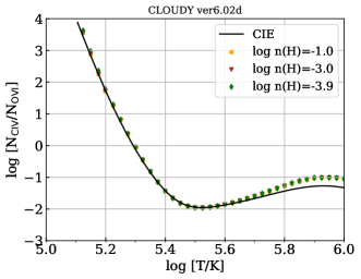
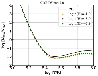
Typically, all of the observed line transitions cannot be reproduced with one phase of gas. It is often the case that a model that fits the low-ionization transitions (e.g., Mg ii, Fe ii) cannot produce the observed amount of high-ionization absorption (e.g., C iv, O vi), or adequately match the profiles of the full Lyman series. In such cases, we will use more than one optimized ion. The other optimized ions represent the different phases of gas, with distinct regions having different densities along the line-of-sight. For example, we would typically optimize on Mg ii for the low-ionization gas, and on C iv for high-ionization gas. In some intervening absorbers, O vi, because of its comparatively high ionization potential ( 114 eV), arises in gas with T 105 K where the ionization is governed by collisions between energetic free electrons and metal ions (Pradeep et al. 2020). We model the gas phase traced by O vi to be under collisional ionization equilibrium (CIE). For such collisional ionization models, the cloudy grids are run over space: [-3.0,1.5] and [5.0, 5.8]. Similar to the PIE modeling, the CIE models are obtained by varying the total column density of hydrogen, , until the column density of O vi is matched for each point on the grid. In Figure 1, we show for a metallicity of and different gas densities that cloudy can produce accurate results when modeling gas in CIE. The column density ratios of C iv/O vi agree well with the CIE model (Gnat & Sternberg 2007) for temperatures in the range of K, and are independent of the hydrogen number densities. We contrast the modeling results obtained with cloudy ver6.02d and ver17.01 to show that the apparent discrepancy with the Gnat & Sternberg (2007) model arises because of the evolving atomic database (Chatzikos et al. 2015). The cloudy models are generated for an assumed value of , based on the Milky Way halo density at 50kpc (Kaaret et al. 2020).
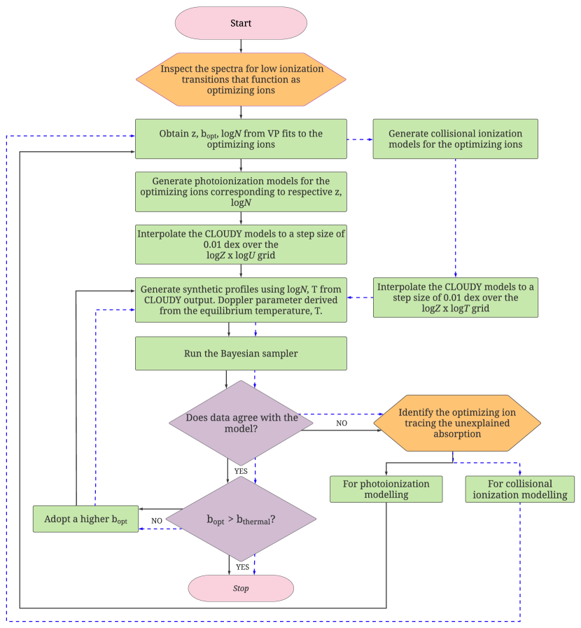
To summarize, we start with the assumption that a single, low ionization phase describes an absorption system. If such a simple, one-phase model fails to account for the observed column densities in all the transitions, we incorporate additional phases until the synthesized spectra from cloudy best match the observed spectra for all transitions. Generally, we find that a single phase is insufficient to explain the observed abundances of all the transitions even when the transitions coincide in velocity space. If the synthetic spectra fit the data for all transitions, then it is plausible that the physical conditions in the cloudy model match those in the gas that produces the absorption. This allows us to determine precise allowed ranges of metallicity, density, and temperature for each individual cloud that create the observed transition lines. A summary of the methodology is given in the form of a flowchart in Figure 2.
4 RESULTS
4.1 Application to four quasar absorption line systems
We discuss the findings from the application of our methodology to four, weak low-ionization absorption line systems, and compare our results to those obtained from earlier studies adopting the HM12 model for the EBR.
4.2 The absorber towards the quasar PHL1811
| Lyman lines | Ly-only | ||||||||||||
| Optimized | |||||||||||||
| ion | (km s-1) | (km s-1) | |||||||||||
| (1) | (2) | (3) | (4) | (5) | (6) | (7) | (8) | (9) | (10) | (11) | (12) | (13) | (14) |
| C iii0 | 0.07766 | 5.0 | |||||||||||
| Si iii0 | 0.07774 | 3.1 | |||||||||||
| Si iii1 | 0.07779 | 5.7 | |||||||||||
| O vi0 | 0.07770 | 47.0 | - | - | - |
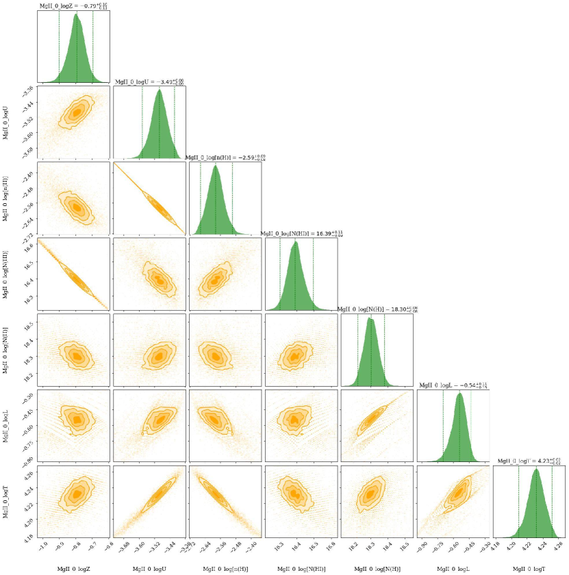
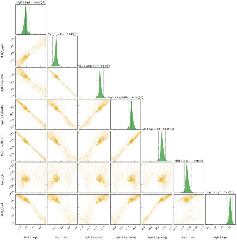
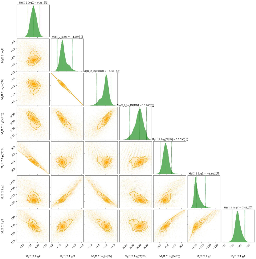
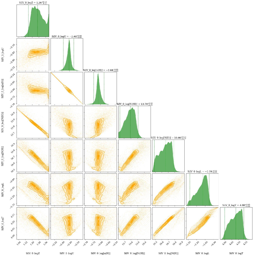
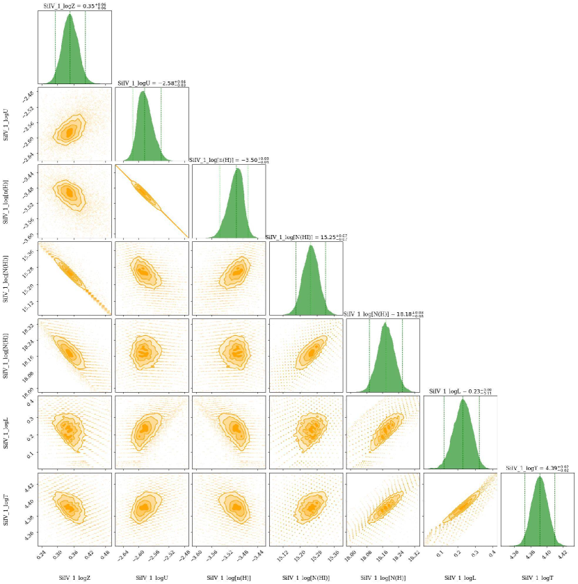
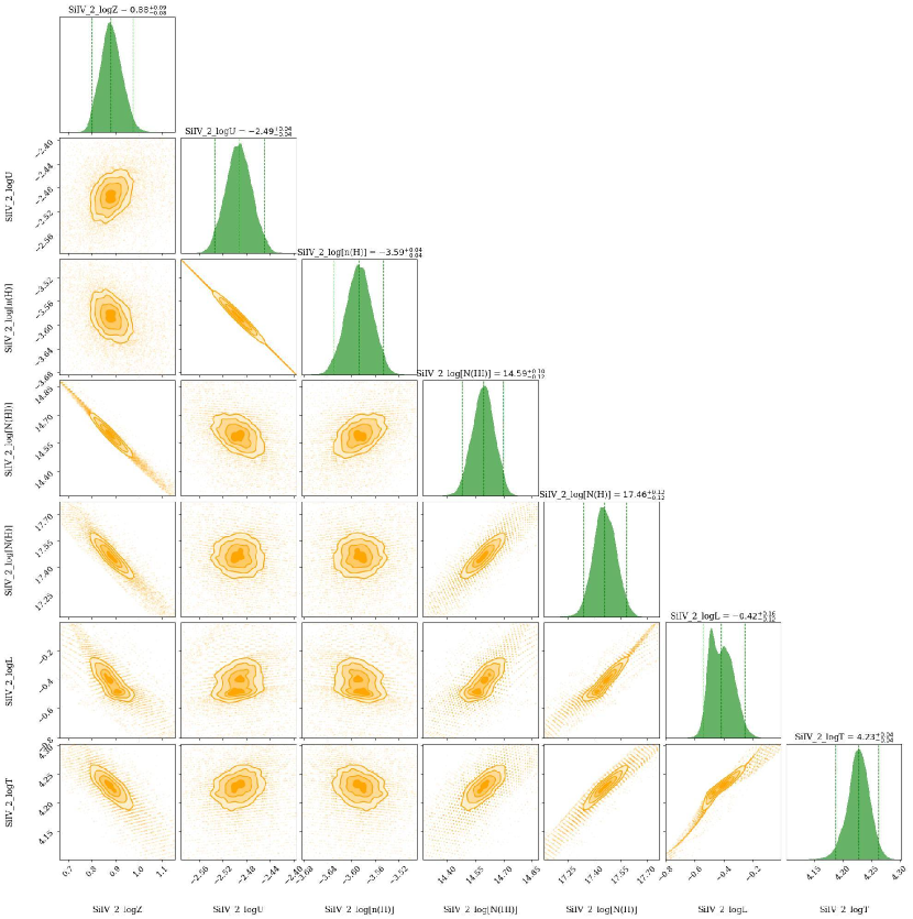
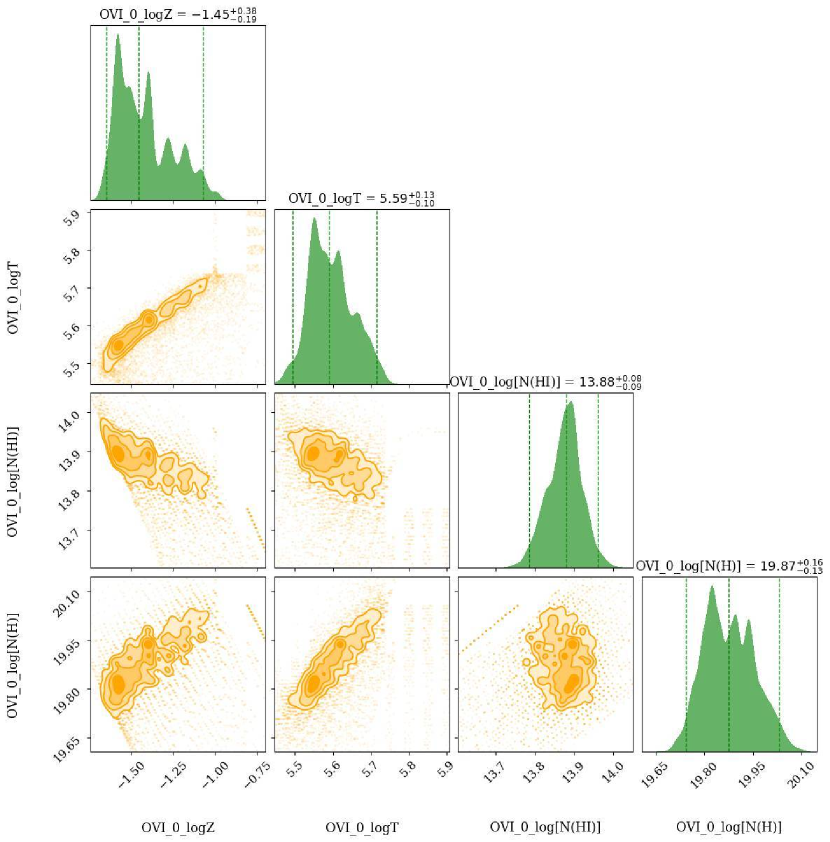
Properties of the different gas phases contributing to the absorber towards PHL1811 traced by their respective optimized ions. Notes: (1) Optimized ion tracing a phase; (2) Redshift of the component; (3) Doppler parameter of optimized ion; (4) Adopted Doppler parameter for the optimized ion; (5) log column density of optimized ion; (6) log metallicity; (7) log ionization parameter; (8) log hydrogen number density; (9) log hydrogen column density (10) log thickness in kpc; (11) log temperature in Kelvin. The marginalized posterior values of model parameters are given as the median along with the upper and lower bounds associated with a 95% credible interval. For the collisionally ionized O vi phase, the quantities and are not determined as they are dependent on the assumed value of . The synthetic profiles based on these models are shown in Figure 3. The marginalized posterior distributions for the VP fit parameters (columns 2, 3, and 5) of the optimized ions are presented in Figures 15, 16, and 17. The marginalized posterior distributions for the cloud properties (columns 6, 7, 8, 9, 10, 11) are presented in Figures 18, 19, 20, and 21. Columns (12), (13), and (14) describe the marginalized posterior distributions of log metallicity, log ionization parameter, and log hydrogen column density, for a Ly-only model described in § 4.2.2.
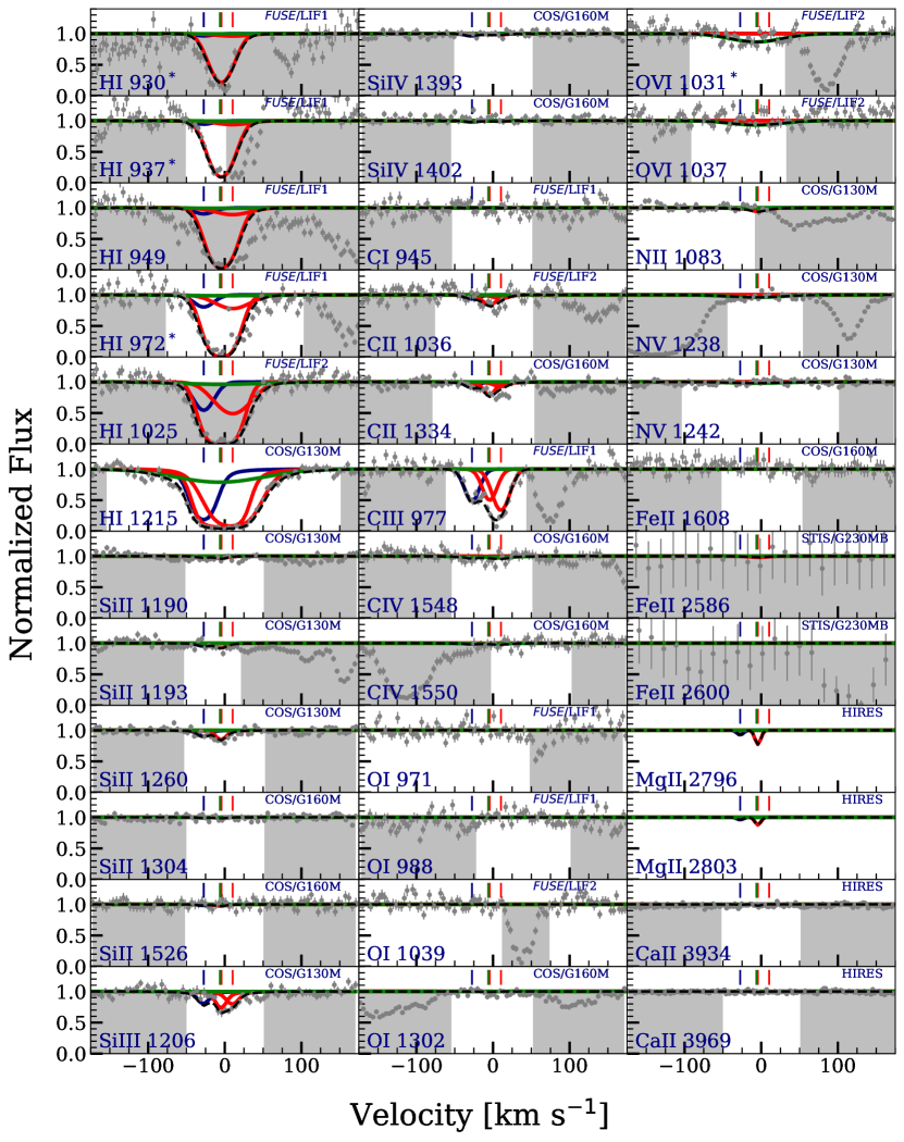
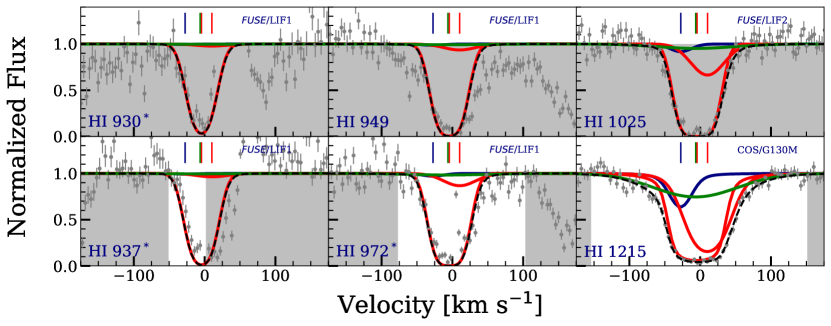
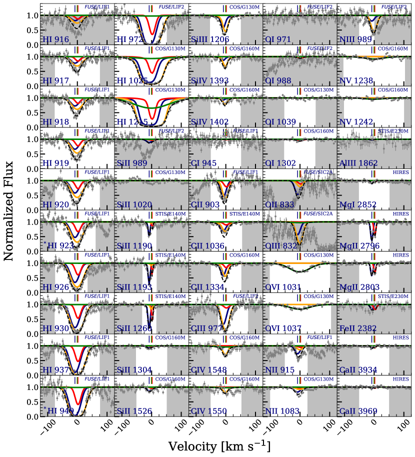
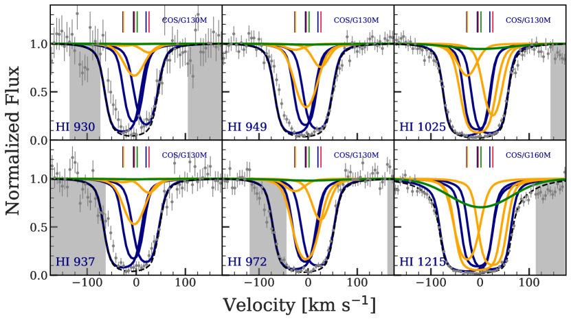
A system plot of the absorber, with the constraining transitions shown, is given in Figure 3. This system has weak absorption detected in Si ii and C ii. Though Mg ii is not covered in the STIS/G230MB spectrum, it is expected to be weak as well. The Fe ii, covered in the COS/G160M and STIS/G230MB spectra, is not detected. The intermediate ionization transitions, Si iii and C iii, are detected, however, Si iv and C iv are not detected. The O vi is detected in the 1031 transition, but not in the 1037 transition. O vi 1031 is contaminated at km s-1 by Galactic Fe ii 1112. We account for the contribution of Fe ii 1112 using other Galactic Fe ii lines from COS data, and display the corrected O vi 1031 profile. The Ly transition was covered by /COS observations, however, all constraining higher order Lyman series lines plotted (down to H i 930) come from FUSE observations. The lines H i 937, and H i 930 are affected by contamination due to the Galactic molecular hydrogen lines. H i 937 is affected by H W 80 Q(2)1010.94 at 59 km s-1, and H i 930 by H L 80 P(1)1003 at 26 km s-1. We divide out the contribution due to these blends using several of the Galactic hydrogen molecular lines present in the FUSE observations. The lines H L 60 R(0) 1024.37 and H L 61 R(1) 1024.99 affect the continuum placement of H i 949 on its redward side. We omit H i 949 as a constraining ion. The H i 972 is blended at 10 km s-1 with Galactic Ar i 1048; we divide out its contribution to the H i 972 profile using the Ar i 1066 line. The Ly is strongly contaminated by Galactic Si iii 1205 (Savage et al. 2014), and though the contamination is at the center of the saturated profile, Ly is still not used as one of the constraining transitions.
We begin by optimizing on the column density of C iii for the blueward cloud and Si iii for the redward cloud. We find that the VP fit to C iii yields a large uncertainty on its -parameter ( km s-1). The best-fit cloudy model for the C iii cloud corresponds to , , and . However, this temperature is too high to be consistent with the best VP fit -parameter for C iii. We therefore tried a 2 higher -parameter (b(C iii) = 7.00 km s-1) for the C iii cloud and found the temperature () to be considerably lower because of the resulting higher metallicity (). We find a similar high value of metallicity for a -parameter only 1 higher than the best fit value ((C iii) = 5.00 km s-1). In Table 2 we present the model with (C iii) = 5.00 km s-1.
For the redward Si iii cloud we find that a single component fit results in overproduction of Ly and underproduction of C iii on the redward side of the profiles. An adjustment of the of the optimized Si iii cannot resolve both of these discrepancies. A two component fit is thus preferred for Si iii, and the column densities and Doppler parameters for the optimized Si iii are listed in Table 2. Again, we found that the best VP fit -parameters for the two Si iii components resulted in a model with a temperature too high to be self-consistent. Therefore, we adopt 1 higher values for the -parameters of the two redward components in Si iii. The posterior distributions for , and for the C iii and two Si iii components are presented in Figures 15 and 16. For the redward cloud, the lower ionization Si ii and C ii transitions might have been used as optimized transitions, however the VP fits would be quite uncertain due to their noisier profiles. Also, C iii is affected by line saturation, so Si iii is the best choice for the optimized transition for the redward cloud. It is clear that the ionization parameters of the three low ionization clouds must be relatively low, since Si iv and C iv are not detected, such that O vi could not be produced in the same phase with the C iii and Si iii. We therefore determine that this absorber is best explained by invoking the presence of a high ionization phase giving rise to the O vi absorption. The VP fit posterior distribution for O vi is presented in Figure 17.
In Table 2 we present the posterior results for the low ionization phase, which are summarized in Figures 18, 19, and 20 for the C iii component and the two Si iii components, respectively. Figure 3 shows cloudy models, using the maximum likelihood estimate (MLE) values superimposed on the data. These plots show that the metallicities of the two redward components (red curve) are constrained to be and in order to fit the Ly profile, and several of the Lyman series transitions. The metallicity of the weaker, blueward C iii component is constrained to be , and it fits the blue wing of Ly in combination with the middle Si iii cloud and the O vi cloud.
Table 2 summarizes the constraints placed on the metallicities, ionization parameters, number density of hydrogen, values, thickness, and temperatures for the two low ionization clouds. The blueward cloud has a thickness of 6 pc, and the two redward clouds have thicknesses of 35 pc and 0.5 kpc respectively. The three clouds fall far short of producing a partial Lyman limit break (combined ).
This low ionization phase does not produce O vi absorption. While it is possible that the absorption is a broad Ly component unrelated to the detected broad O vi absorption, a collisionally ionized phase, such as a Coronal Broad Lyman-alpha Absorber (CBLA; Richter 2020), optimized on O vi, is also consistent with the data. This CBLA would have a temperature of , so as not to produce detectable C iv absorption, and to fit the wings of the Ly line. For km s-1, the wings of Ly are fit for a metallicity of . The posterior results for this high ionization phase are summarized in Figure 21.
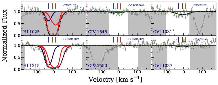
We also investigate the alternative of a photoionized phase in O vi. A photoionized model with and a supersolar metallicity could fit the O vi profile, and also well explains the observed abundances of other transitions, however the blueward wing of Ly is unexplained as shown in Figure 4. A model with lower ionization parameter could fit the wing of Ly but would overproduce the C iv. Hence, we favor a collisional ionization model for the O vi phase.
4.2.1 Comparison to Previous Models
Our modeling reveals three components seen in the low ionization transitions, and required by the observed profiles. The responsible photoionized clouds are found to differ from each other in metallicity, from 1/10th solar metallicity to highly supersolar. There is also a separate, collisionally ionized phase () that produces broad O vi and H i absorption. The total H i column density from our model is .
Lacki & Charlton (2010) conducted multiphase modeling for this system, using a wider grid of and , and the HM01 (Haardt & Madau 2001) EBR. Also, C iv appears to be detected in the /STIS spectrum that they used, which we do not detect in our /COS coverage. For the blueward cloud in C iii, they determine and producing C iv and O vi. In contrast to their metallicity, we find with a lower ionization parameter of such that C iv is not produced. We find that a low metallicity, , with our lower ionization parameter, would yield a high temperature phase that violates equation 3.
For the redward low ionization absorption, they find a single low metallicity value of and . In agreement with their result, we determine two separate low metallicities of and with ionization parameters of and , respectively.
Other recent models for this system find average values using a single, low ionization component. Keeney et al. (2017) found and , using , and using the same HM12 as we have. Muzahid et al. (2018) measured and, using the KS15 (Khaire & Srianand 2015) EBR, found and . In our models, the centered Si iii cloud has a similar metallicity, and produces nearly all of the absorption in higher order Lyman series lines because of its larger H i column density. The redward Si iii cloud is, however, essential to producing the Ly absorption in the base of the profile, and is thus required to have a lower metallicity. Our conclusions regarding the presence and properties of a collisionally ionized O vi phase contributing to this system are consistent with those of Savage et al. (2014) who determine and [O/H] = .
4.2.2 Caveats and Tests
Though we do not have wavelength coverage of the key Mg ii transition in any of our spectra for this quasar, we do show the predicted profiles from our favored model in Fig. 3. The Mg ii would most likely classify as a single component, weak Mg ii absorber with mÅ. Only the blueward Si iii cloud produces detectable Mg ii, though we do see a slight contribution from the C iii cloud.
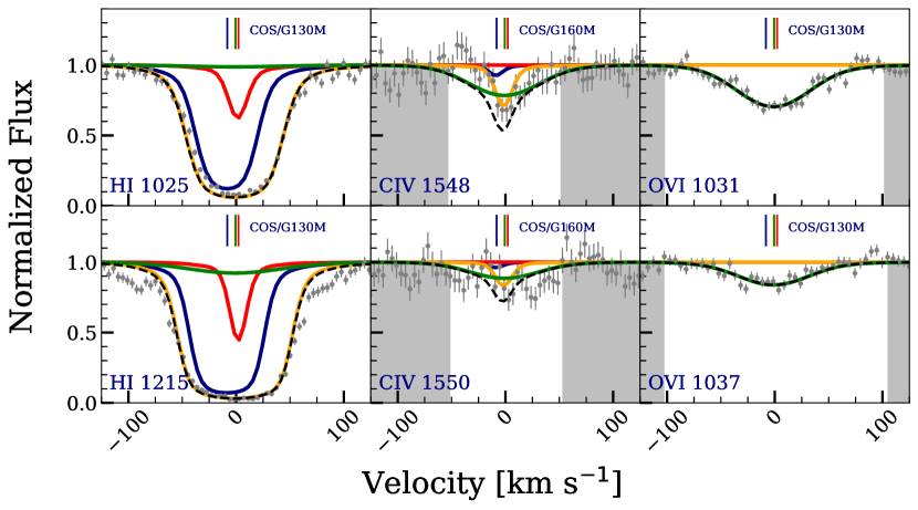
The four systems we have chosen to model in this paper, demonstrating our methodology, have richer datasets than the typical low weak, low ionization absorber (Muzahid et al. 2018). Most importantly, in many cases there is no FUSE coverage of the Lyman series lines. To see what the effect would be on constraints, we have run our models considering only the Ly line. Table 2 lists the constraints from this experiment. We find the values for and to be consistent, for all four clouds, with our model that makes use of all the Lyman series coverage. There is, however, a large uncertainty in the values for the “Ly only” model, particularly for the blueward C iii cloud. The “Ly only” model is shown in Fig. 5. The ability to constrain parameters using only Ly is important given that many of the systems in the literature only have one to two H i lines, and thus the robustness of the method to limited H i data is very important.
As another test of our methodology, we synthesized artificial spectra modeled after this absorber. We add Gaussian noise to the modeled flux of the synthetic spectra, and flux uncertainties are based on the average observed in that part of the spectrum. We included one blueward C iii cloud, two blended Si iii clouds and a warm/hot O vi cloud, as we found for this absorber. For our experiment, we adopted four different sets of metallicity, , and ionization parameter, values, including a combination similar to the real system shown in Figure 6. These parameter choices for our simulations are listed in Table 3 along with the recovered values. In two cases we altered the metallicities in the synthetic spectra, and in one other case we adjusted the ionization parameter of the blueward C iii and the blended redward Si iii clouds while keeping the parameters of O vi cloud fixed at the values of the best fit model. In all cases we were able to recover the correct model parameters, with the errors, that we specified for the synthetic spectra. This provides confidence that our CMBM approach is recovering accurate results from the observed spectra.
| Simulated | Recovered | ||||
|---|---|---|---|---|---|
| Test ID | Phase | ||||
| A | C iii | ||||
| Si iii | |||||
| Si iii | |||||
| B | C iii | 0.10 | |||
| Si iii | 0.10 | ||||
| Si iii | 0.10 | ||||
| C | C iii | ||||
| Si iii | |||||
| Si iii | |||||
| D | C iii | ||||
| Si iii | |||||
| Si iii |
The results of testing the algorithms’ ability to recover the information of simulated spectra. Test A corresponds to a synthesized spectrum with the parameters determined for the absorber towards PHL1811. The models superimposed on the data are shown in Figure 6 for Test A. Test B, C, and D correspond to different combinations of metallicity and ionization parameter; in all the cases we are able to recover expected values within the errors.
The final consideration for this absorber is the relatively large uncertainties in the VP fit parameters for the blended optimized Si iii clouds and for the C iii cloud. The best VP fit for the Si iii yielded km s-1 for the blueward component and km s-1 for the redward component, and for C iii we found km s-1, as noted in Table 2. The photoionization models based on these best VP fit parameters for the blueward C iii, and the two redward Si iii produce high temperatures that are not self-consistent with equation 3. We resolved the problem by adopting higher values within the limits of 2 uncertainty. If we did adopt the best VP fit parameters, cloudy models would find consistent values of and for the Si iii clouds, but would find a drastically lower metallicity (of ) for the C iii cloud. This indicates that in the absence of higher resolution coverage of an optimized transition, there is some level of systematic uncertainty in the derived model parameters. The possible effects of different values of blended components should always be considered.
4.2.3 Galaxy Properties and Physical Interpretation
The closest galaxy to the sightline, at a coincident redshift, is a quiescent, inclination , galaxy at an impact parameter of 237 kpc (Keeney et al. 2017). It is unlikely that the galaxy itself would produce significant absorption for impact parameters 200 kpc (Liang & Chen 2014), however Muzahid et al. (2018) notes that there are 7 galaxies within 1 Mpc and 500 km s-1 of the absorber. This suggests a group environment.
Only one of the three low ionization clouds in this system, the middle one with , would produce detectable weak Mg ii absorption. With a metallicity of , and a size of pc, it is consistent with the weak, low ionization absorber population at intermediate redshift Rigby et al. (2002); Charlton et al. (2003); Misawa et al. (2008). However, those absorbers often have a lower density, C iv phase aligned in velocity with the Mg ii. The blueward cloud is also very small and has a supersolar metallicity. The redward cloud, however, has a lower metallicity of , and a larger line-of-sight thickness of pc. This cloud would be consistent with lines of sight through infalling gas in filamentary structures as seen in numerical simulations (Hafen et al. 2019). It is unclear if the three clouds are structurally related, despite their close proximity in velocity space.
Because of the lack of detected C iv, this absorber is similar to the well studied Virgo cluster absorber found toward 3C 273 (Stocke et al. 2004). Though they are not common (Milutinović et al. 2006), there is reason to believe that the lower amplitude EBR will lead to some systems with less prominent C iv absorption (Narayanan et al. 2005). In this absorber, though C iv is not detected, we do see collisionally ionized gas giving rise to O vi absorption, a transition not often covered for the higher redshift systems. A survey of low redshift, weak low ionization absorbers is needed to see if such warm/hot gas is commonly found, perhaps arising in an intragroup medium, such as it is observed in the Local group (Bouma et al. 2019), or at the interface between cooler clouds and hotter surrounding regions (Oppenheimer et al. 2016; Pointon et al. 2017).
4.3 The absorber towards the quasar PHL1811
| Lyman lines | Ly-only | ||||||||||||
| Optimized | |||||||||||||
| ion | (km s-1) | (km s-1) | |||||||||||
| (1) | (2) | (3) | (4) | (5) | (6) | (7) | (8) | (9) | (10) | (11) | (12) | (13) | (14) |
| C iii0 | 0.08057 | 12.0 | |||||||||||
| C iv0 | 0.08074 | 12.0 | |||||||||||
| C iv1 | 0.08092 | 13.0 | |||||||||||
| Si ii0 | 0.08092 | 5.00 |
Properties of the different gas phases present in the absorber towards PHL1811 traced by their respective optimized ions. Notes: (1) Optimized ion tracing a phase; (2) Redshift of the component; (3) Doppler parameter of optimized ion; (4) Adopted Doppler parameter for optimized ion; (5) log column density of optimized ion; (6) log metallicity; (7) log ionization parameter; (8) log hydrogen number density; (9) log hydrogen column density (10) log thickness in kpc; (11) log temperature in Kelvin. The marginalized posterior values of model parameters are given as the median along with the upper and lower bounds associated with a 95% credible interval. The synthetic profiles based on these models are shown in Figure 7. The marginalized posterior distributions for the VP fit parameters (columns 2, 3, and 5) of the optimized ions are presented in Figures 22, 23, and 24. The marginalized posterior distributions for the cloud properties (columns 6, 7, 8, 9, 10, and 11) are presented in Figures 25, 26, 27, and 28. Columns (12), (13), and (14) describe the marginalized posterior distributions of log metallicity, log ionization parameter, and log hydrogen column density, for a Ly-only model described in § 4.3.2.
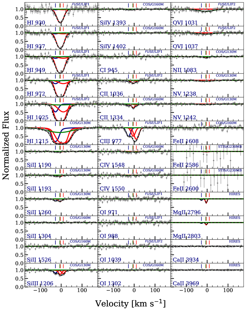
Spectral regions covering constraining transitions for the absorber, from FUSE, /COS, /STIS, and Keck/HIRES, are shown in Fig. 7. The low ionization absorption in Si ii and C ii shows two components, with the redward being the strongest. The system might classify as a multiple component weak Mg ii absorber, but the Mg ii transitions were not covered to confirm that expectation. The H i 1025, H i 972, H i 949, and H i 937 are affected by blending due to the Galactic molecular hydrogen lines. H i 1025 is contaminated by H:L 00 R(1) 1108.63 at km s-1, H i 972 by H:L 40 P(1) 1051.03 at km s-1 and by H:L 40 R(2)1052.49 at 56 km s-1, H i 949 by H:L 60 R(2)1026.53 at km s-1, and H i 937 by H:L 70 R(1)1013.44 at km s-1. We divide out the contribution of these lines by making use of several other Galactic hydrogen molecular lines observed in the FUSE spectrum.
This system was previously analyzed by (Jenkins et al. 2003; Jenkins et al. 2005; Richter et al. 2016; Richter 2020). The strongest low ionization component is also detected in O i, N ii, Fe ii, and Ca ii. There are three components detected in C iii, and the two redward components in C iv as well. In a noisy part of the FUSE spectrum, O vi provides only an upper limit. Lyman series lines, from Ly down to H i 920, provide useful constraints on the metallicities of the three components, with the blueward component clearly separated in the higher order lines. The metallicity of the strongest, redward component is best constrained by the redward side of all the Lyman series profiles. A full Lyman break is observed at this redshift in the FUSE coverage (Jenkins et al. 2003). Table 4 summarizes the constraints placed on the metallicities, ionization parameters, number densities, neutral hydrogen column densities, temperatures, and thickness for the four clouds we find necessary to explain the multiphase absorption.
Since C iii is saturated for the strongest component, and several Si ii lines were covered, the model is optimized on the measured Si ii column density. This cloud was constrained to have metallicity, , and gives rise to the Lyman limit break. It also fits the distinctive “wing” on the redward side of the Ly profile, and also produces a small amount of absorption consistent with the smaller “wing” on the blueward side. For an ionization parameter of , the observed O i, Fe ii, and N ii are fully produced, but all the higher ionization transitions are underproduced, calling for a separate, higher-ionization phase at this same velocity. The Ca ii was not included as a model constraint because it is often depleted onto dust (Richter et al. 2011), and we do find it to be overproduced by 0.75 dex by the model. The large needed to reproduce this relatively strong profile results in a cloud thickness of 1.7 kpc.
To account for the C iv, S iv, C iii, Si ii, N iii, and C ii, coincident with the strongest Si ii component, we included an additional cloud, optimized on the C iv at this velocity. This cloud has the highest ionization parameter of among the absorbers present in this system, this cloud can produce the observed absorption in all these transitions. Its metallicity must be relatively high (we obtain ) in order that it does not affect the fit to the Lyman series lines. The thickness of this cloud is kpc.
For the middle component, the optimized transition is C iv, since the C iii is saturated, and detections are weak or absent in the low ionization transitions. This cloud has an ionization parameter of . A metallicity of allows this cloud to fill in the Lyman series profiles in between the contributions from the other clouds, which themselves are well constrained from the blueward and redward sides of the profiles. Despite its much lower of 15.5, relative to the strongest cloud, the low metallicity leads to a similar cloud thickness of 63 kpc. This model, however, overpredicts the absorption in N iii, but an abundance pattern variation from solar could resolve this discrepancy.
The third, blueward cloud model is optimized on C iii since it is at most weakly detected in Si ii and C ii. Because C iv is not detected, this cloud has a lower ionization parameter of . A supersolar metallicity () is required in order that Lyman series lines are not overproduced. Though the is similar to that for the middle cloud, the thickness is several orders of magnitude smaller, only 5 parsecs. This contrast in thickness is striking, and perhaps surprising, but it seems to be required by the observed profiles.
In Table 4 we present the posterior results for different phases, which are summarized in Figures 25, 26, 27, and 28 for the four clouds.
4.3.1 Comparison to Other Models
It is apparent from our models that the four clouds needed to explain the low ionization absorption profiles have significantly different properties from one another, pointing to different physical origins of the gas. The metallicities of these clouds are found to be for the strongest low ionization component, for the coincident higher ionization component, a very low metallicity of for the middle cloud, and for the weak, blueward component. The redward, strong low ionization component also contributes the bulk of the H i absorption and produces a Lyman limit break, as well as giving rise to the wings on the Ly profile. Richter (2020) has modeled the right, broad wing of the Ly absorption as CBLA that traces the collisionally ionized, coronal gas of the CGM host galaxy, however, we find that the wing is explained by the redward Si ii cloud.
The middle cloud has , while the redward cloud has . Another startling difference is perhaps the thicknesses of the clouds, with the lower density, high metallicity cloud that is only 5 pc thick, while the redward spans a few kpc.
Previous models by Keeney et al. (2017), Muzahid et al. (2018), and Wotta et al. (2019) which average the components together infer metallicities and ionization parameters consistent (considering differences in EBR models) with those we obtain for the strongest lower ionization component. However, they miss the richness of information available in the profile about two other regions along the sightline which have vastly different properties and physical origins.
4.3.2 Caveats and Tests
| 0.9T | T | 1.1T | ||||
|---|---|---|---|---|---|---|
| Phase | ||||||
| C iii_0 | ||||||
| C iv_0 | ||||||
| C iv_1 | ||||||
| Si ii_0 |
The results of testing the influence of possible uncertainties in cloudy equilibrium temperature on model parameters. We find that a 10% change in temperature from the value given by cloudy still produces qualitatively similar results.
For this system, we predict the strength of Mg ii. The equivalent width predicted for Mg ii is mÅ, dominated by the redward cloud.
We also conduct a test for this system to determine how much information can be derived using a “Ly only” model. Table 4 summarizes these constraints for the “Ly only” model compared to the original one. Even without access to the Lyman series lines, the ionization parameters and metallicities of all but the middle C iv clouds agree well within errors. This disagreement arises due to the fact that the higher order lines provide the information necessary to produce the shape of the profile. The “Ly-only” model is shown in Fig. 8.
Central to our ability to discern accurate model parameters, even from saturated H i lines, is the use of the cloudy model equilibrium temperature in order to determine the thermal/turbulent contributions to the parameter, and thus to infer for each component. We thus investigated for this system the effect of uncertainties in the temperature given by cloudy, considering values 10% smaller and 10% larger for all four clouds. In order to do this, for each cloudy model we took the output temperature and artificially adjusted it before synthesizing model spectra. When these model spectra, which therefore were produced with different parameters for non-optimized transitions, were compared to the data, different and parameters were found to compensate for the different values. Results are summarized in Table 5. This table shows that the effects of this assumed uncertainty are quite small. As expected, we find that a lower temperature will lead to a larger thermal contribution and a larger , and thus a slightly smaller inferred metallicity, while a higher temperature will lead to a slightly larger metallicity. Results are overall not very sensitive to the equilibrium cloudy temperatures.
4.3.3 Galaxy Properties and Physical Interpretation
The closest galaxy to the sightline at this redshift is an early type galaxy at an impact parameter of 35 kpc from the sightline (Keeney et al. 2017). Although the Sloan survey does not show many other galaxies within 1 Mpc and 500 km s-1 of the line of sight (Muzahid et al. 2018), there is one close companion galaxy with at an impact parameter of 87 kpc (Jenkins et al. 2005), which is possibly interacting with the nearer galaxy.
Our inference of four very different gas clouds points toward there being different processes at work along the sightline. The presence of two nearby galaxies suggests that there could be gas associated with each of the two different galaxies, or with debris that resulted from their interaction. There also could be gas associated with the group of galaxies containing the pair and also possibly dwarf galaxies to these L∗/ sub-L∗ galaxies, though no other bright galaxies are present besides the two.
It is very interesting that the smallest of the four clouds is a fairly typical, supersolar, weak, low ionization absorber. These are typically not associated closely with specific galaxies, however in this case there is a galaxy within an impact parameter of 35 kpc. The lowest metallicity cloud () could be gas infalling into the galaxy pair from a more pristine surrounding environment, consistent with expected values for IGM accretion metallicities from simulations, which yield values between (Hafen et al. 2019). In this case, there is no evidence of hot gas that produces broad O vi absorption, consistent with the previous studies of group environments (Oppenheimer et al. 2016; Pointon et al. 2017). Instead, the wings of the Ly profile can be fully explained by the low ionization cloud that produces a full Lyman break.
4.4 The absorber towards the quasar PG1116+215
| Lyman lines | Ly-only | ||||||||||||
| Optimized | |||||||||||||
| ion | (km s-1) | (km s-1) | |||||||||||
| (1) | (2) | (3) | (4) | (5) | (6) | (7) | (8) | (9) | (10) | (11) | (12) | (13) | (14) |
| Mg ii0 | 0.13846 | 2.9 | |||||||||||
| Mg ii1 | 0.13850 | 1.7 | |||||||||||
| Si iv0 | 0.13847 | 6.0 | |||||||||||
| O vi0 | 0.13848 | 34.7 | - | - | - |
Properties of the different gas phases present in absorber towards PG1116+215 traced by their respective optimized ions. Notes: (1) Optimized ion tracing a phase; (2) Redshift of the component; (3) Doppler parameter of optimized ion (4) Adopted Doppler parameter for the optimized ion (5) log column density of optimized ion; (6) Metallicity; (7) log ionization parameter; (8) log hydrogen number density; (9) log hydrogen column density (10) log thickness in kpc; (11) log temperature in Kelvin. The marginalized posterior values are given as the median along with the upper and lower bounds associated with 95% credible interval are given. For the collisionally ionized O vi phase, the quantities and are not determined as they are dependent on the assumed value of . The synthetic profiles based on these models are shown in Figure 9. The marginalized posterior distributions for the VP fit parameters (columns 2, 3, and 5) of the optimized ions are presented in Figures 29, 30, and 31. The marginalized posterior distributions for the cloud properties (columns 6, 7, 8, 9, 10, and 11) are presented in Figures 32, 33, 34, and 35. Columns (12), (13), and (14) describe the marginalized posterior distributions of log metallicity, log ionization parameter, and log hydrogen column density, for a Ly-only model described in § 4.4.2.
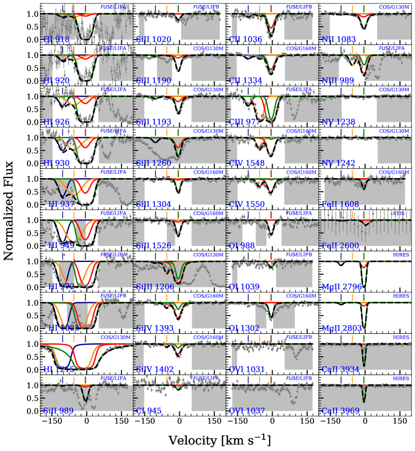
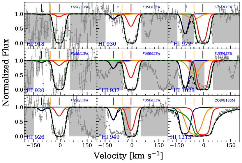
Keeney et al. (2017) have modeled this absorber using /COS, /STIS, and FUSE spectra and determine a metallicity of for a single, low ionization cloud in this absorber. However, the higher resolution, Keck/HIRES data reveals the presence of two narrow components in Mg ii ( and km s-1) with = 95 5 mÅ. It is important to note that relatively broad (820 km s-1) low ionization components may often resolve into narrower components (17 km s-1), and the parameters of these components can substantially affect the constraints on the metallicity in our modeling method. Several of the lines from the system are affected by blends with other systems along the sightline. The H i 949 and H i 923 are affected by the Galactic molecular hydrogen lines. The H i 949 is contaminated at km s-1 by H L 2–0 P(2) 1081.265, and H i 923 at km s-1 by H L 4–0 P(1)1051.03. We divide out the contribution of these lines using the several other Galactic hydrogen lines observed in the FUSE spectrum. The H i 972 line is contaminated by the Ly of absorber at km s-1, and the H i 926 line is contaminated by Ly of the absorber at km s-1. We mask their influence in the log-likelihood evaluation.
The low ionization Mg ii clouds in this absorber are also detected in N ii, Si ii, C ii, and Mg i and marginally in Ca ii and O i. The O ii is contaminated by H W 30 R(3)948.42, but the profile is still shown for completeness in Figure 9. The region of the /STIS spectrum covering Fe ii 2382 is too noisy to provide a useful constraint. The intermediate ionization states, Si iii, O iii and C iii are detected (though O iii is contaminated by H L 140 R(2)948.47), and though it is not as strong as the Mg ii, C iv is also detected. These transitions are clearly offset by km s-1 redward of the low ionization transitions. A broad, O vi cloud is clearly detected in both doublet members, in the high /COS spectrum. The Ly and Ly were covered in the high /COS spectrum as well, but the higher order Lyman series lines, down to 918, were covered by FUSE. It is critical to note that the H i lines appear to be centered on the Si iv and C iv absorption rather than on the low ionization absorption. These velocity offsets suggest that two phases are needed to fit this system.
Our modeling yields constraints presented in Table 6, and model curves that are superimposed on the data in Figure 9. The posterior distributions for the parameters are summarized in Figures 32, 33, 34, and 35 for the different phases. The parameter (=2.9 km s-1) adopted for the blueward Mg ii cloud is higher than the best VP fit value, because the lower value yielded a cloudy model temperature too high to be consistent with the line width. The two, narrow, low ionization clouds have high metallicities ( and , low ionization parameters ( and ), low temperatures (104 K and 103.0 K), and small thickness (100 pc and 1 pc). With these low ionization parameters, only a small fraction of the intermediate ionization absorption can arise in the same phase as the low ionization absorption. It is also impossible to produce the Ly and other H i lines with such narrow low ionization clouds, particularly the redward cloud which is best fit with of only 1.7 km s-1.
A slightly broader cloud optimized on the Si iv column density ( km s-1) was added to the model and a maximum likelihood solution is determined combining with the two low ionization clouds, and an additional broad O vi cloud to be discussed below. This Si iv cloud produces the majority of the Si iii absorption and all of the observed C iv absorption. It also produces the majority of the Ly absorption and a substantial fraction of the Lyman series lines as well. The properties of this Si iv cloud are , , and cloud thickness of kpc, and it contributes to the model.
In Figure 9, the model, including the three low ionization clouds, slightly overproduces the observed C ii 1036, but it is apparently consistent with the C ii 903 and 1334 lines, so we assume there may be a small defect in the C ii 1036 data. The results are not dependent on which of the C ii transitions are used as constraints.
The broad O vi cloud ( km s-1) is consistent with collisional ionization with , and it can produce the wings on the Ly line that would otherwise be unexplained. The metallicity to provide that fit to Ly is .
We also test if O vi could arise in a photoionized phase. A photoionized model with and a supersolar metallicity could fit the O vi profile, without contributing to the H i however it also produces a broad C iv profile which is clearly inconsistent with the data, as shown in Figure 10.
4.4.1 Comparison to Previous Work
This system might have been fit with just one low ionization component if it were not for higher resolution and high coverage of Mg ii, which clearly shows two narrow components. These clouds are typical of weak Mg ii absorbers at higher redshifts (-), with low ionization parameters and , super solar metallicities ( and ), and small thickness (100 pc and 1 pc). Our modeling indicates the presence of two additional phases in order to produce the observed high ionization and H i absorption, which cannot come from the low ionization clouds. An intermediate ionization phase, with and with low metallicity () produces Si iii, Si iv, and C iv absorption and is responsible for the majority of H i absorption as well, having . This intermediate ionization gas phase is much more extended, with a thickness of kpc. Finally, broad O vi absorption and wings on the Ly profile constrain the properties of a higher ionization/hotter phase. We find it to be consistent with collisional ionization at in line with the Ly fit by Stocke et al. (2014) (=86 11 km s-1). Richter (2020) successfully fitted an even broader component to the combined STIS and COS data set (=150 km s-1). He identified the extended wings of the Ly profile as part of a CBLA that traces the collsionally ionized, hot coronal gas of the host galaxy of this CGM absorber, in line with the predicted CBLA properties from his semi-analytic model (Richter 2020; Sect. 5.5). In contrast, Savage et al. (2014) inferred a lower temperature of , and a contribution from photoionization from their analysis. However, we find that O vi arising in a photoionized phase gives rise to a broad C iv which is inconsistent with the data, as shown in Figure 10.
Previous investigators (e.g. Keeney et al. 2017; Muzahid et al. 2018; Pointon et al. 2019; Wotta et al. 2019) found metallicities () intermediate between those of our low metallicity, intermediate ionization cloud, and our supersolar metallicity, low ionization clouds. The ionization parameters of these earlier models tend to match that of our intermediate ionization phase, with , because they are trying to produce all the absorption in a single phase. We see a significant variation in ionization parameter/density across the profiles. Again the possible origin of the absorber through a combination of low metallicity inflowing gas, and high metallicity outflowing gas, may be smeared out through modeling that does not consider multiple components and phases.
4.4.2 Caveats and Tests
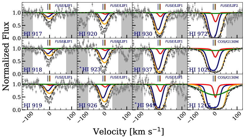
For this system, a “Ly only” model provides constraints that qualitatively match those that we obtained with the full model. These constraints, with errors, are compared in Table 6. The best “Ly only” model slightly under predicts several of the higher order H i lines because of the slightly lower metallicity for the Si iv phase. The “Ly only” model is shown in Figure 11.
4.4.3 Galaxy Properties
There are three galaxies within an impact parameter of 1 Mpc at the redshift of this absorber (Muzahid et al. 2018), with the nearest being an galaxy at an impact parameter of 139 kpc (e.g. Keeney et al. 2017). As with the previous systems, this absorber appears to be found in a small group of galaxies.
The low ionization clouds are again typical of the supersolar metallicity, parsec-scale, weak Mg ii absorbers that are pervasive at intermediate redshifts Rigby et al. (2002); Narayanan et al. (2008). The Si iv cloud is more characteristic of a sightline through the larger, intragroup medium, since it is 60 kpc in extent along the sightline, and has a low metallicity. It would presumably be gas falling into the group (Hafen et al. 2019), because of its low metallicity of . The warm/hot, collisionally ionized O vi phase also has a relatively low metallicity of . Perhaps this gas is more related to the nearest galaxy, or perhaps to an unidentified dwarf in the group, or to the low-metallicity coronal gas of the absorber host galaxy.
4.5 The absorber towards the quasar HE0153-4520
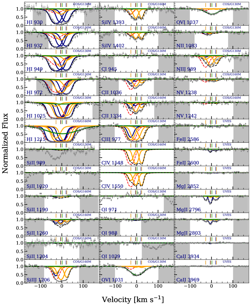
This three component, weak Mg ii absorber (with mÅ) also shows absorption in the low ionization Si ii, C ii, N ii, and Fe ii transitions. Because the Mg ii is observed with the highest resolution with VLT/UVES, it is used as the optimized transition in our modeling. The detection of Fe ii, in particular, requires a low ionization parameter/high density for the two blueward, low ionization clouds. Because of this, the detected Si iii, C iii, N iii, and Si iv cannot be produced in the same phase. Our model thus also includes three intermediate ionization clouds, optimized on the Si iv doublet. Finally, a strong detection of broad O vi absorption and the corresponding wings in the Ly profile call for a high ionization, collisionally ionized gas phase for the absorber, possibly related to a CBLA that traces the hot halo of the host galaxy.
Thus, our optimized cloudy models are run incorporating seven clouds in three phases. The VP fit parameters for the three components identified in Mg ii which traces the low ionization phase, the three component fit for the S iv which traces the intermediate ionization phase, and the single component fit for the O vi tracing a collisionally high ionization phase are given in Table 7, along with the model parameters. The marginalized posterior distributions for the VP fit parameters are shown in Figures 36, 37, and 38. The marginalized posterior distributions for the physical properties of clouds are shown in Figures 39, 40, 41, 42, 43, 44, 45.
Our first attempt to fit this system revealed a discrepancy in fitting the C iii profile with the three clouds optimized on Si iv, with the left side of the C iii profile underproduced and the right side overproduced. Though a wavelength shift of the C iii profile (within errors in calibration) could have explained this discrepancy, that is not likely because the Lyman series lines at similar wavelengths were not similarly shifted. Instead, we found that adjusting the parameters of the Si iv components, within the errors in our VP fit, could match the C iii profile, because the C iii is highly dependent on on its flat part of the curve of growth. Our adopted values of for our final model are listed as a separate column in Table 7.
The three low ionization clouds have metallicities ranging over an order of magnitude. The blueward cloud, which has and does not give rise to Fe ii absorption has in order to fit the left side of the Lyman series profiles. The thickness of this cloud is 300 pc. The redward Mg ii cloud, with and , is unusually broad, with km s-1, and we note that if there were two narrower components in its place then the metallicity value could be significantly lower. Thus the metallicity of this cloud is a bit uncertain. The middle Mg ii cloud also has a low value of because of detected Fe ii, and a solar metallicity, with a relatively large uncertainty of 0.2 dex because of being in the center of the Lyman series profiles. Because of their low ionization parameters and high densities (), the two redward Mg ii clouds must be quite thin (only pc).
Most of the H i absorption does arise in the low ionization phase, with a total of from the three clouds. This agrees with the depth of a partial Lyman limit break, observed in the FUSE data (Savage et al. 2011).
The three intermediate ionization clouds, optimized on Si iv, have similar constraints on , corresponding to a density of . For these ionization parameters, the observed weak N v absorption is produced in these clouds. They also must all have supersolar metallicities in order that they do not exceed the Ly absorption. Since the low ionization clouds that are producing the bulk of the Ly absorption, there is not much room for a contribution to the H i column density from these intermediate ionization clouds. They are larger, with thicknesses ranging from 100 pc to 1.7 kpc. In Figure 12, we show a model (red dashed curve) with solar metallicity in Si iv_0 cloud which exceeds the absorption seen in Ly, C ii, C iii, N iii, and N v.
The collisionally ionized, high ionization phase is found to fit the broad O vi profiles and the wings on the Ly profile with and . For this temperature, very little N v absorption is produced, which is necessary since the N v arose primarily in the Si iv clouds.
| Lyman lines | Ly-only | ||||||||||||
| Optimized | |||||||||||||
| ion | (km s-1) | (km s-1) | |||||||||||
| (1) | (2) | (3) | (4) | (5) | (6) | (7) | (8) | (9) | (10) | (11) | (12) | (13) | (14) |
| Mg ii0 | 0.22585 | 7.9 | |||||||||||
| Mg ii1 | 0.22594 | 7.7 | |||||||||||
| Mg ii2 | 0.22604 | 15.3 | |||||||||||
| Si iv0 | 0.22585 | 12.0 | |||||||||||
| Si iv1 | 0.22594 | 9.8 | |||||||||||
| Si iv2 | 0.22606 | 7.0 | |||||||||||
| O vi0 | 0.22597 | 34.9 | - | - | - |
Properties of the different gas phases present in absorber towards HE0153-4520 traced by their respective optimized ions. Notes: (1) Optimized ion tracing a phase; (2) Redshift of the component; (3) Doppler parameter of optimized ion; (4) Adopted Doppler parameter for the optimized ion (5) log column density; (6) Metallicity; (7) log ionization parameter; (8) log hydrogen number density; (9) log hydrogen column density (10) log thickness in kpc; (11) log temperature in Kelvin. The marginalized posterior values with the median along with the upper and lower bounds associated with 95% credible interval are given. For the collisionally ionized O vi phase, the quantities and are not determined as they are dependent on the assumed value of . The synthetic profiles based on these models are shown in Figure 12. The marginalized posterior distributions for the VP fit parameters (columns 2, 3, and 5) of the optimized ions are presented in Figures 36, 37, and 38. The marginalized posterior distributions for the cloud properties (columns 6, 7, 8, 9, 10, and 11) of absorbers present in this system are shown in Figures 39, 40, 41, 42, 43, 44, 45. Columns (12), (13), and (14) describe the marginalized posterior distributions of log metallicity, log ionization parameter, and log hydrogen column density, for a Ly-only model described in § 4.5.2.
4.5.1 Comparison to Previous Work
This system has three distinct absorption phases, two photoionized with high densities of cm-3 in the low ionization phase, and values much lower in the intermediate ionization phase. The metallicities of the low ionization clouds range from to around the solar value, while those of the intermediate ionization clouds must be supersolar. The collisionally ionized, high ionization cloud has a temperature of K, and a metallicity of .
Previous models (e.g. Savage et al. 2011; Muzahid et al. 2018; Wotta et al. 2019) derived values of metallicity for the low ionization gas ranging from to , depending on the assumed EBR. At face value, an average of would result from our three separate clouds, however we have noted that there is uncertainty in the redward clouds, and also the value would tend to be lower if a different EBR besides HM12 was assumed as in the other models.
The temperature of our collisionally ionized phase of K is considerably less than the value of over a million degrees which Savage et al. (2011) derived from the ratio of the measured parameters of O vi and H i from VP fitting. We find that a lower temperature, and a lower parameter of km s-1 is more consistent with the shape of the Ly profile when combined with the contributions from the other gas phases.
4.5.2 Caveats and Tests
We again tried the experiment of considering what constraints would be in the absence of coverage of the Lyman series lines. Table 7 summarizes the results. The two models closely agree in their ionization parameters and metallicities, with the important exception of the blueward, low ionization cloud. The metallicity of this cloud for the “Ly- only” model is , as compared to for our full model. This much lower metallicity predicts , as compared to a contribution of in our full model. It is already clear that this is incorrect because we do not observe a full Lyman break from this system. Thus it is not surprising that the “Ly only” model over predicts the higher order Lyman series lines.
We now consider the reason for this discrepancy. Without the constraints from the Lyman series, the wing of the Ly profile on the blueward side is filled in by the blueward, low ionization cloud, rather than a broad Ly component related to the broad O vi absorption. The higher order Lyman series lines, starting at H i 949, make it clear that such a model would overproduce the H i absorption on the blueward side as shown in Figure 13. Despite this change, the inference of the metallicity and temperature of the collisionally ionized phase is not significantly different between the two models.
It is clear that the model that utilizes all the constraints of the Lyman series lines is more accurate, however, we still note that the Ly line alone does give some very important and correct conclusions. Even with just the Ly we can see that two of the low ionization clouds and all three high ionization clouds have solar or higher metallicity. It is also clear that all six of these clouds, and a broad O vi cloud, must exist in order to fit the data.
We show in Figure 12 the expected C iv absorption, contributed by the intermediate ionization clouds for this system. If we had coverage of C iv in the observed spectrum then the constraints on these clouds would be quite secure.
4.5.3 Galaxy Properties and Interpretation
This absorber is at an impact parameter of 80.2 kpc from a luminous () galaxy (Keeney et al. 2018). However, in this case, a dozen galaxies are found within an impact parameter of Mpc and a velocity of km s-1, suggesting a rich group environment.
This rich galaxy environment would be consistent with the relatively strong O vi absorption associated with collisionally ionized gas, at the boundary between the low ionization layers and the surrounding hot medium Pointon et al. (2017). The low ionization absorption is produced in higher density gas than in the previous absorbers. These very condensed (sub-parsec) structures may be enriched fragments originating in outflows McCourt et al. (2012). In this case, the intermediate ionization phase, giving rise to the Si iv absorption (and predicted strong C iv absorption) in three clouds, seems to be well-aligned in velocity with the low ionization clouds. This would suggest a similar origin for the two phases, perhaps with a higher density collapsed region within a lower density region giving rise to the intermediate ionization absorption. This would also be feasible in winds from dwarf galaxies, which could plausibly produce the high metallicity seen in the intermediate ionization clouds (Fujita et al. 2020).
5 DISCUSSION
As a test of our methodology, we have applied our CMBM method to four, well-studied, weak, low ionization absorbers. These systems are the absorber towards the quasar PHL1811, the absorber towards the quasar PHL1811, the absorber towards the quasar PG1116+215, and the absorber towards the quasar HE0153-4520.
Constraints from our modeling of the four system are given in Tables 2, 4, 6, and 7. Our best fit models for the four systems are superimposed on the observational data in Figures 3, 7, 9, and 12.
5.1 Metallicity constraints from cloud-by-cloud, multiphase, Bayesian modeling
In all four cases we were able to find an adequate fit, with one to four different phases, to all covered radiative transitions. Since metallicity is crucial to interpretations, we summarize, in Figure 14, the constraints we have placed on the metallicities of each component for the four systems, with each component labeled with the optimized transition for our model, and plotted in velocity space to show the kinematic structure of the system. The results for the individual components are compared to a single value that we derive from averaging our individual components, weighted by and plotted at km s-1. These values are also compared to constraints on metallicity placed by previous investigators (Lacki & Charlton 2010; Savage et al. 2011; Keeney et al. 2017; Muzahid et al. 2018; Pointon et al. 2019; Wotta et al. 2019). Note that there will be differences of 0.4 dex (for e.g., between HM05 and HM12) in the metallicity derived from models based on their adoption of different EBR amplitudes and shapes (Wotta et al. 2019). We are, however, concerned only with the general, qualitative results that affect our gross interpretations. The sizes of the points in Figure 14 are in proportion to the thickness of the clouds from our models. We notice the following trends:
1. In three of the four cases (all but the absorber towards HE0153-4520) our mean, -weighted, metallicity agrees with those derived in previous studies, taking into account differences in the EBR.
2. In the absorbers at and towards PHL1811 our inferred, mean value is dominated by the strongest, low ionization cloud. However, in the other two cases, several clouds, spanning more than two orders of magnitude in metallicity, strongly influence the mean value.
3. Generally, low ionization phase clouds have high inferred metallicities. In two cases, the absorber towards PHL1811 and the absorber towards HE0153-4520, intermediate ionization (Si iv and C iv) clouds have even higher metallicity values.
4. For the absorber towards HE0153-4520, the values from previous investigations are an order of magnitude smaller than the -weighted mean from our study. This is due to the two supersolar metallicity Mg ii clouds.
5. In the three absorbers with detected O vi, the broad O vi profiles can be explained by collisionally ionized gas, which also in all cases makes an important contribution to Ly absorption in the wings of the profile (as so-called CBLAs), possibly tracing hot coronal gas and which would otherwise be difficult to explain. In all three cases the metallicity of the collisionally ionized gas is consistent with .
6. In all four cases, the averaging of the metallicities of components and phases, hides important variations along the profile. For example, supersolar metallicities in some of the components could be a signature of outflowing gas or patchy distribution of metals. Similarly, low metallicities seen in other components could indicate an origin in pristine, inflowing gas. It should not be surprising that multiple processes are contributing along the same sightline, which is likely to have contributions to absorption from regions spanning a couple hundred kiloparsecs.
The CMBM method allows us to dissect the system into these different components. Because of this refinement, it should be much more likely that trends with galaxy properties will be revealed if modeling is performed on a larger sample of galaxies/absorbers. For example, in Pointon et al. (2019), no correlation was seen between system metallicity and the inclination and azimuthal angle of the nearest galaxy. This was surprising because there is an expectation that there will be a higher metallicity along the minor axis due to outflows, and a lower metallicity along the major axis where gas inflowing from the surrounding environment is seen. This expectation is confirmed by an analysis of the IllustrisTNG and Eagle cosmological hydrodynamic simulations by Peroux et al. (2020). Examining possible correlations between the highest and lowest metallicity components of our observed systems could reveal trends that have previously been disguised, and resolve this discrepancy. There is already an indication of a relationship between metallicity and azimuthal angle using dust ([Zn/Fe]) as a proxy, in a sample of 13 galaxy/Mg ii pairs (Wendt et al. 2020).
5.2 Strengths and limitations of cloud-by-cloud, multiphase, Bayesian modeling
Generally, for these four weak, low ionization absorbers, we demonstrate that our method is successful in extracting the physical conditions (ionization parameters and metallicities) of the various regions of gas along a sightline.
In § 4 of this paper, we gave details of how each model parameter was constrained by specific observed transitions (e.g., if the metallicity of this cloud was any lower, the left side of the Ly and Ly profiles would be overproduced). This lends confidence to the accuracy of the results, within the context of our assumptions about the phase structure. Similarly, we have considered whether our formal error bars seem reasonable. For example, in Figure 12 we have shown that a solar metallicity for component Si iv_0 is clearly discrepant as it overproduces Ly, C ii, C iii, N iii, and N v to the blue, thus showing that this component must have a highly supersolar metallicity value.
To test the robustness of our method, we designed a simple test to see if we could recover the input parameters of synthetic spectra. The synthetic spectra were based on the parameters that we derived for the system towards PHL1811, as listed in Table 3, with an example shown in Figure 6. For all four synthetic spectra, with a range of metallicities and ionization parameters, we were able to separate the C iii cloud and two Si iii clouds and infer their different metallicities, within errors. We are also able to correctly infer the ionization parameters, if they are similar as in the observed system, or if they are different as in our simulated spectra Test C (Table 3). This builds confidence that we are correctly determining that clouds along the same line of sight, even in the same phase, can have very different densities, metallicities, or thickness.
For weak, low ionization absorbers, including the four in our sample, the Ly is often on the flat part of its curve of growth. That makes it impossible to derive an accurate measurement of via a VP fit. In Muzahid et al. (2018), Table 2 shows that many of the values are quite uncertain for a larger sample of similar systems from which these four were drawn. Despite this limitation, it is possible to obtain meaningful constraints on the metallicity of the absorbing clouds. Our method relies on the more accurate measurement of the -parameters of the different components for the optimized metal ion. From these parameters, and using the temperatures from cloudy, we can calculate the thermal/turbulent fractions, and derive the value of for each component. One can use the parameter of a metal line to infer the parameter of an H i component. By doing so one can break the degeneracy of VP fitting to even just the Ly line and derive accurate metallicities, particularly for the redward and blueward, low ionization components. Interplay between the low and intermediate ionization phases, and even contributions to the wings of Ly from the high ionization phase, must be incorporated into the Bayesian optimization. However, even with just a low ionization phase, there is a very strict lower limit on the metallicity derived from the requirement that the left and right sides of the Ly profile are not overproduced.
We emphasize that breaking the degeneracy of measuring on the flat part of the curve of growth is essential to our method. As a result, it is critical that the parameters of the optimized transitions are accurate, and are not uncertain either due to low resolution observations or to component blending. We must be aware of the possibility that the best VP fit value for a given optimized transition might result in a cloudy model temperature that is inconsistent, and in such a case the adopted parameter for the optimized transition should be increased. Our method also assumes that the equilibrium temperature from cloudy is accurate, and that discrete, constant density, cloud structures are an adequate approximation for the absorbing gas. We considered the effect of a possible 10% error in the equilibrium temperature, and found it to have negligible effect on inferred metallicity values. We can also test these assumptions in the following way. In these four absorbers we typically have access to four or five clean (not blended) Lyman series lines in addition to the Ly, and in two cases there is coverage of the Lyman break, allowing an accurate and direct constraint on the total . For all four systems we blindly ran our entire CMBM method on the data including the metal lines, but only using Ly and not the higher order Lyman series lines. Despite this limitations, in all cases we were able to correctly infer the metallicity of the dominant component, and in all but one of the systems we extracted qualitatively similar values for all the absorbing cases. Figures 5, 8, 11, and 13 show how closely the remaining Lyman series models were predicted by our “Ly-only" models.
Of course, when many Lyman series lines are covered we have great confidence that we will accurately derive the metallicities of all of the components. A straightforward way to infer that multiple phases are needed for some systems is to note that a single component fit cannot adequately explain both the shape of the Ly line and the strengths of the higher order Lyman series lines. Narrow, low ionization clouds often account for the higher order Lyman series lines, while broader, intermediate ionization clouds are often needed to match the base/edge of the Ly and Ly lines. It also appears that broader, high ionization lines are required to explain the wings of the Ly profile. These wings, which seems to be common in these types of systems, possibly indicate the contribution of the hot coronal gas halos of the galaxies to the Ly absorption (CBLAs; Richter 2020). They do provide, in any case, an important way to determine if photoionization or collisional ionization is dominant for the high ionization phase that produces the O vi absorption. For example, this provided evidence to favor collisional ionization, instead of photoionization, for the O vi in the system towards PHL1811 and in the system towards PG1116+215.
Just as the H i lines often call for significant contributions from different phases, some metal lines, particularly those with intermediate ionization, also require such contributions. Once the phase structure is determined, and the optimized transitions are set as input, our method can formally adjust the balance of these phases to produce the best fits to the profiles of all specified transitions.
With the inferred model parameters it is possible to predict the line profiles of all radiative transitions, even those that were not covered in the data available. This can predict, for example, whether a system is indeed likely to be a weak Mg ii absorber even in cases like the two absorbers towards PHL1811 for which wavelength coverage of that doublet was not available. This allows comparisons to other systems in the same class.
The true power of CMBM method cannot be realized unless there is a way of passing beyond spending weeks laboring over the details of each individual system. This automated Bayesian approach makes it possible to cover all of parameter space in a systematic and automated manner, once the cloud and phase structure are specified. Building on the experience gained by modeling other systems of the same type, it is expected that most systems can be fully explored within roughly a day. This puts systematic studies of tens or even 100 absorption systems within reach, which is crucial to compare different absorption properties in the different phases to each other, and to the luminosities, morphologies, and orientations of the absorbing galaxies.
Though there are clear advantages to our methodology, which represents clear progress over previous studies, there are still some limitations, and aspects which require careful attention to individual systems. Determination of the minimum phase structure that adequately describes an absorber is an iterative process and does require some human intervention. For example, the low ionization phase can contribute to the intermediate phase absorption, but may not fully produce it. This contribution would have to be taken into account if an intermediate phase transition is used as an optimized transition, and the optimized column density reduced. In such a case the low ionization phase properties would need to be fixed in the modeling process. Also, it is important to recognize blends with our constraining transitions, and to eliminate the proper regions before running the program. A discrepancy with a spurious region of spectrum in a single transition can dominate and be a determining factor in model parameters.
Furthermore, though we strive to find an adequate model using the minimum number of phases, such a model is not unique. It is always possible that an additional phase contributes, and that there is an alternative solution that is equally plausible. In such a case, predicting additional transitions, or predicting structure in existing observations at higher can provide a helpful way to distinguish between such models should new data acquisition prove possible.
There is also a limit to conclusions that can be drawn if a variety of radiative transitions, with varying ionization states, are not covered. Since our method relies on using the parameter of a metal-line transition to determine , and since this is essential to determining metallicity constraints, it is important that at least one metal-line transition in each phase is covered at high resolution and , and is unsaturated. For example, for the absorber toward PG1116+215 the coverage of Mg ii clearly shows two components. If we only had coverage of the Si ii with /COS resolution we would have tried to fit the system with only one component in place of the two. We faced this challenge in our modeling of the absorber toward PHL1811, where high resolution ground-based data were not available covering Mg ii or Fe ii because of the low system redshift. In this case, we were able to infer that there were likely two blended, narrower components fitting the Si iii, however, the advantages of this two-component model were subtle, and some of the model parameters depended on the specific VP fit assumed for the Si iii. This warns us to be cautious to consider the implications of splitting an unresolved component into two when we do not have high resolution coverage. We also noted above, that though “Ly only” models often provide reliable constraints, it is also possible that some values, especially for weak clouds, will be inaccurate, as we saw in Figure 7 for the absorber towards PHL1811.
We simply must be aware of such limitations when not as many transitions have been covered, and our Bayesian optimization can take these systematic uncertainties into account when deriving the range of allowed parameters. Even if transitions are missing coverage, so that an intermediate or high ionization phase is missed, we can still derive lower limits on the low ionization gas phase metallicity.
The systems in this study do not have coverage of different elements contributing in the same phase to allow meaningful constraints on abundance pattern. Sometimes more transitions are covered, e.g. ions of O and C spanning several ionization states. When this is the case, it is possible to extract some basic information about abundance pattern, such as the elevated C/O ratio found in Yadav et al. (in preparation).
For absorbers that lie within 100 kpc of the star-forming disk of the CGM host galaxies, the local galaxy radiation most likely plays a role. For the Milky Way, Richter et al. (2009); Bouma et al. (2019) have included the local disk radiation field in their cloudy modeling and have discussed this issue in detail and give a perspective what should be done when modeling the photoionization in CGM clouds. We don’t incorporate the effects of nearby galaxies as it is beyond the scope of the current study.
A practical limitation on the CMBM method is the need for significant computing power. The number of cloudy models per component in order to construct the required grid, is 2700. Every such model takes an average of 5 minutes of compute time on Intel (R) Xeon (R) CPU E5-2650 v4 2.20GHz. Even these relatively simple absorbers have 3-7 components in the different phases, and a stronger, low ionization absorber might have several times more. A serial job would take between 28-65 days to obtain the models covering the desired parameter space. Additionally, the need for more exact UV radiation field models including the contribution from the local galaxy disks, would further complicate the modeling and substantially increase the computation time. To generate these cloudy models in a reasonable amount of time, it is important to employ parallel processing methods. Our parallel implementation of generating cloudy models makes use of the in-house CyberLAMP cluster infrastructure.
5.3 Application to understanding weak, low ionization absorbers
The focus of this paper has been a demonstration of the CMBM methodology. We chose to apply it to four, previously well-studied, weak, low-ionization absorbers. As we described in § 1, this population of absorber is of particular interest because of their high metallicities despite locations far from known galaxies. In the future, we intend to apply these methods to a systematic determination of the gas phase properties of the larger sample of 34 absorbers from Muzahid et al. (2018). However, it is still of interest to consider any general conclusions that we can draw about the population based on the properties of these four absorbers in our present study.
We have concluded that:
1) All of the four low ionization weak absorbers have low ionization clouds that must have solar or supersolar metallicities.
2) Of the clouds that produce low ionization (Mg ii or Si ii) absorption, six of them have densities, , in the range to , two of them have , and two have much higher densities of as constrained by detected Fe ii absorption.
3) Depending on their densities and metallicities, the line-of-sight thickness of the low ionization clouds range from a fraction of a parsec up to a few hundred parsecs, with typical values of a few to tens of parsecs. The thickness constraints for the different clouds are shown as symbol sizes in Figure 14.
4) Only one of the absorbers ( toward HE0153-4520) has a distinct and separate intermediate ionization phase aligned with the low ionization clouds in velocity space. These intermediate ionization clouds have densities of and thickness of 100 pc to 1 kpc. Though it is not covered by spectra, we would expect strong C iv absorption from this system based upon its model properties. Such phase structure is typical of , weak Mg ii absorbers, and is envisioned as sheetlike or filamentary higher density structures embedded in or adjacent to lower density structures.
5) Three of the absorbers have evidence of multiple galaxies in the fields, indicating a group environment (Jenkins et al. 2005; Keeney et al. 2017; Muzahid et al. 2018). The fourth absorber, toward PHL 1811, is found at 35 kpc from a 0.56 galaxy that is within tens of kpc of another galaxy, and could plausibly be interacting.
6) Three of the four absorbers have a collisionally ionized phase giving rise to broad, O vi absorption. It is interesting to note that the case without O vi is the case of the lower impact parameter, interacting galaxy candidate, which has no evidence of a larger, group environment. In our larger study, we will investigate the hypothesis that warm/hot O vi could be a characteristic of the group environment.
7) In three of the four absorbers we find compelling evidence for broad H i components in the Ly profile that point to collisionally ionized gas that either is related to the broad O vi or traces an even hotter gas component, the million-degree coronal gas halo (Richter 2020). Our multi-phase Bayesian modelling provides a powerful method to identify such Coronal Broad Ly Absorbers (CBLAs) even in complicated, multi-phase CGM absorbers and thus could be of great help for future, systematic studies of CBLAs in low-redshift galaxies.
Considering the population of weak, low ionization absorbers at low redshift, we note that many of these absorbers do appear to arise in gas in a narrow density range around , and from gas with a solar or supersolar metallicity. However, we also note that for gas structures with this density, the column density of low ionization transitions scales directly with the metallicity. Thus if the gas in this density range was in a small structure or if it had a significantly subsolar metallicity it would be unlikely to be detected in low ionization absorption. If this population of weak, low ionization absorbers are dominated by gas of this density, we would expect a bias towards high metallicities in our sample. Since these absorbers are commonly observed they must have a large covering factor, and it is still necessary to explain the mystery of the pervasive nature of such high metallicity gas far from galaxies. However, we also should consider that lower metallicity gas of this same density will likely exist as well, and we should learn to recognize its absorption signatures. Finally, we note that some of the gas that might exist in that same density range at would tend to have stronger C iv absorption and weaker (or undetected) Mg ii absorption. Our larger, systematic study of weak, low ionization absorbers will consider the redshift evolution of different populations of gas clouds.
Surely, weak, low ionization absorbers (as with any class of absorbers) have multiple physical origins, and can arise in gas with various combinations of densities and metallicities. Furthermore, it is always important to remember that the same population of gas clouds is traced by a different population of absorbers at different redshifts, because of the evolution of the EBR, as well as the evolving processes contributing to the gas conditions. Finally, many different populations of absorption systems are observed at all redshifts, and these are all connected to one another. The complexity of this situation, and the variety in absorption systems, make it urgent that we explore the physical conditions of the absorbers in a detailed, yet automated way. We have demonstrated in this paper, with our application to four absorbers and associated tests, that such a study is now possible.
6 Conclusion and Future Work
Our CMBM method provides great detail about the physical conditions, metallicities and densities, of absorption systems. We have applied the method to four well-studied weak low-ionization absorbers, and demonstrated its power in deriving accurate results, and estimating realistic uncertainties for the physical properties of the gas. This tool has similar potential for studies of absorbers of all types, and for larger samples of absorbers given its semi-automated nature, and its computational efficiency. By separating the multiple gas phases, in a larger sample, we can explore possible relationships between metallicity, density, phase structure, and temperature of the circumgalactic medium, with galaxy properties such as impact parameter, luminosity, orientation, and galaxy environment.
This methodology hinges on using the Doppler parameters of metal lines to constrain the Doppler parameters of H i lines, thus breaking degeneracies in the curve of growth, and separating out the contributions to the Ly and Lyman series lines from multiple phases of gas. It is particularly effective when there are at least some radiative transitions observed with high spectral resolution, and when there is high quality data covering many different metal-line transitions as well as many Lyman series lines. Because of this, we expect the method will transfer well to samples of Lyman break and partial Lyman break systems at various redshifts. In future work, we plan to apply this CMBM method to several large samples of systems in order to obtain a much more rigorous understanding of the complex and multiple processes at work in the circumgalactic medium.
ACKNOWLEDGEMENTS
We thank the anonymous referee for their insightful review which improved the quality of the paper. Computations for this research were performed on the Pennsylvania State University’s Institute for Computational and Data Sciences’ Roar supercomputer. J.C.C., S., J.M.N, and C.W.C. acknowledge support by the National Science Foundation under grant No. AST-1517816. G.G.K. and N.M.N. acknowledge the support of the Australian Research Council through Discovery Project grant DP170103470. Parts of this research were supported by the Australian Research Council Centre of Excellence for All Sky Astrophysics in 3 Dimensions (ASTRO 3D), through project number CE170100013. S.M. is supported by the Alexander von Humboldt Foundation, Germany, via the Experienced Researchers Fellowship. We acknowledge the work of people involved in the design, construction and deployment of the COS on-board the Hubble Space Telescope, and thank all those who obtained data for the sight-lines studied in this paper.
Data availability
The data underlying this article will be shared on reasonable request to the corresponding author.
References
- Adelberger et al. (2005) Adelberger K. L., Shapley A. E., Steidel C. C., Pettini M., Erb D. K., Reddy N. A., 2005, The Astrophysical Journal, 629, 636
- Anglés-Alcázar et al. (2017) Anglés-Alcázar D., Faucher-Giguère C.-A., Kereš D., Hopkins P. F., Quataert E., Murray N., 2017, MNRAS, 470, 4698
- Barber et al. (1996) Barber C. B., Dobkin D. P., Huhdanpaa H., 1996, ACM Transactions on Mathematical Software (TOMS), 22, 469
- Bergeron (1986) Bergeron J., 1986, Astronomy and Astrophysics, 155, L8
- Bergeron & Boissé (1991) Bergeron J., Boissé P., 1991, Astronomy and Astrophysics, 243, 344
- Bordoloi et al. (2011) Bordoloi R., et al., 2011, ApJ, 743, 10
- Bordoloi et al. (2014) Bordoloi R., et al., 2014, The Astrophysical Journal, 796, 136
- Borthakur et al. (2015) Borthakur S., et al., 2015, ApJ, 813, 46
- Bouché et al. (2012) Bouché N., Hohensee W., Vargas R., Kacprzak G. G., Martin C. L., Cooke J., Churchill C. W., 2012, MNRAS, 426, 801
- Bouma et al. (2019) Bouma S. J. D., Richter P., Fechner C., 2019, A&A, 627, A20
- Buchner et al. (2014) Buchner J., et al., 2014, Astronomy & Astrophysics, 564, A125
- Charlton et al. (2000) Charlton J. C., Mellon R. R., Rigby J. R., Churchill C. W., 2000, The Astrophysical Journal, 545, 635
- Charlton et al. (2003) Charlton J. C., Ding J., Zonak S. G., Churchill C. W., Bond N. A., Rigby J. R., 2003, The Astrophysical Journal, 589, 111
- Chatzikos et al. (2015) Chatzikos M., et al., 2015, Monthly Notices of the Royal Astronomical Society, 446, 1234
- Chen & Mulchaey (2009) Chen H.-W., Mulchaey J. S., 2009, The Astrophysical Journal, 701, 1219
- Chen et al. (2001) Chen H.-W., Lanzetta K. M., Webb J. K., 2001, The Astrophysical Journal, 556, 158
- Churchill & Charlton (1999) Churchill C. W., Charlton J. C., 1999, The Astronomical Journal, 118, 59
- Churchill et al. (1996) Churchill C. W., Steidel C. C., Vogt S. S., 1996, ApJ, 471, 164
- Churchill et al. (1999) Churchill C. W., Rigby J. R., Charlton J. C., Vogt S. S., 1999, The Astrophysical Journal Supplement Series, 120, 51
- Churchill et al. (2000) Churchill C. W., Mellon R. R., Charlton J. C., Jannuzi B. T., Kirhakos S., Steidel C. C., Schneider D. P., 2000, ApJ, 543, 577
- Churchill et al. (2015) Churchill C. W., Vander Vliet J. R., Trujillo-Gomez S., Kacprzak G. G., Klypin A., 2015, ApJ, 802, 10
- Churchill et al. (2020) Churchill C. W., Evans J. L., Stemock B., Nielsen N. M., Kacprzak G. G., Murphy M. T., 2020, arXiv e-prints, p. arXiv:2008.08487
- Danforth et al. (2016) Danforth C. W., et al., 2016, The Astrophysical Journal, 817, 111
- Danovich et al. (2015) Danovich M., Dekel A., Hahn O., Ceverino D., Primack J., 2015, MNRAS, 449, 2087
- Dekker et al. (2000) Dekker H., D’Odorico S., Kaufer A., Delabre B., Kotzlowski H., Iye M., Moorwood A., 2000, in Proc. SPIE. p. 534
- Ding et al. (2003a) Ding J., Charlton J. C., Bond N. A., Zonak S. G., Churchill C. W., 2003a, The Astrophysical Journal, 587, 551
- Ding et al. (2003b) Ding J., Charlton J. C., Churchill C. W., Palma C., 2003b, The Astrophysical Journal, 590, 746
- Ding et al. (2005) Ding J., Charlton J. C., Churchill C. W., 2005, The Astrophysical Journal, 621, 615
- Ferland et al. (2017) Ferland G., et al., 2017, Revista mexicana de astronomía y astrofísica, 53
- Feroz et al. (2009) Feroz F., Hobson M., Bridges M., 2009, Monthly Notices of the Royal Astronomical Society, 398, 1601
- Ford et al. (2013) Ford A. B., Oppenheimer B. D., Davé R., Katz N., Kollmeier J. A., Weinberg D. H., 2013, Monthly Notices of the Royal Astronomical Society, 432, 89
- Ford et al. (2014) Ford A. B., Davé R., Oppenheimer B. D., Katz N., Kollmeier J. A., Thompson R., Weinberg D. H., 2014, MNRAS, 444, 1260
- Fujita et al. (2020) Fujita A., Misawa T., Charlton J. C., Meiksin A., Mac Low M.-M., 2020, arXiv e-prints, p. arXiv:2009.09954
- Gnat & Sternberg (2007) Gnat O., Sternberg A., 2007, The Astrophysical Journal Supplement Series, 168, 213
- Grevesse et al. (2010) Grevesse N., Asplund M., Sauval A. J., Scott P., 2010, Ap&SS, 328, 179
- Haardt & Madau (2001) Haardt F., Madau P., 2001, in Neumann D. M., Tran J. T. V., eds, Clusters of Galaxies and the High Redshift Universe Observed in X-rays. p. 64 (arXiv:astro-ph/0106018)
- Haardt & Madau (2012) Haardt F., Madau P., 2012, The Astrophysical Journal, 746, 125
- Hafen et al. (2019) Hafen Z., et al., 2019, MNRAS, 488, 1248
- Jenkins et al. (2003) Jenkins E. B., Bowen D. V., Tripp T. M., Sembach K. R., Leighly K. M., Halpern J. P., Lauroesch J. T., 2003, AJ, 125, 2824
- Jenkins et al. (2005) Jenkins E. B., Bowen D. V., Tripp T. M., Sembach K. R., 2005, ApJ, 623, 767
- Johnson et al. (2015) Johnson S. D., Chen H.-W., Mulchaey J. S., 2015, Monthly Notices of the Royal Astronomical Society, 449, 3263
- Jones et al. (2010) Jones T. M., Misawa T., Charlton J. C., Mshar A. C., Ferland G. J., 2010, The Astrophysical Journal, 715, 1497
- Kaaret et al. (2020) Kaaret P., et al., 2020, Nature Astronomy, 4, 1072
- Kacprzak et al. (2008) Kacprzak G. G., Churchill C. W., Steidel C. C., Murphy M. T., 2008, AJ, 135, 922
- Kacprzak et al. (2012) Kacprzak G. G., Churchill C. W., Nielsen N. M., 2012, The Astrophysical Journal Letters, 760, L7
- Kacprzak et al. (2015) Kacprzak G. G., Muzahid S., Churchill C. W., Nielsen N. M., Charlton J. C., 2015, ApJ, 815, 22
- Kacprzak et al. (2019) Kacprzak G. G., Pointon S. K., Nielsen N. M., Churchill C. W., Muzahid S., Charlton J. C., 2019, ApJ, 886, 91
- Keeney et al. (2017) Keeney B. A., et al., 2017, The Astrophysical Journal Supplement Series, 230, 6
- Keeney et al. (2018) Keeney B. A., et al., 2018, The Astrophysical Journal Supplement Series, 237, 11
- Khaire & Srianand (2015) Khaire V., Srianand R., 2015, ApJ, 805, 33
- Krogager (2018) Krogager J.-K., 2018, arXiv preprint arXiv:1803.01187
- Lacki & Charlton (2010) Lacki B. C., Charlton J. C., 2010, Monthly Notices of the Royal Astronomical Society, 403, 1556
- Lanzetta & Bowen (1992) Lanzetta K. M., Bowen D. V., 1992, ApJ, 391, 48
- Lehner et al. (2013) Lehner N., et al., 2013, The Astrophysical Journal, 770, 138
- Liang & Chen (2014) Liang C. J., Chen H.-W., 2014, MNRAS, 445, 2061
- Liang & Remming (2020) Liang C. J., Remming I., 2020, Monthly Notices of the Royal Astronomical Society, 491, 5056
- Lynch & Charlton (2007) Lynch R. S., Charlton J. C., 2007, The Astrophysical Journal, 666, 64
- Martin et al. (2012) Martin C. L., Shapley A. E., Coil A. L., Kornei K. A., Bundy K., Weiner B. J., Noeske K. G., Schiminovich D., 2012, ApJ, 760, 127
- Masiero et al. (2005) Masiero J. R., Charlton J. C., Ding J., Churchill C. W., Kacprzak G., 2005, The Astrophysical Journal, 623, 57
- Massa et al. (2013) Massa D., et al., 2013, COS Data Handbook, HST Data Handbooks
- McCourt et al. (2012) McCourt M., Sharma P., Quataert E., Parrish I. J., 2012, Monthly Notices of the Royal Astronomical Society, 419, 3319
- Milutinović et al. (2006) Milutinović N., Rigby J. R., Masiero J. R., Lynch R. S., Palma C., Charlton J. C., 2006, The Astrophysical Journal, 641, 190
- Misawa et al. (2008) Misawa T., Charlton J. C., Narayanan A., 2008, The Astrophysical Journal, 679, 220
- Murphy (2016) Murphy M., 2016, Uves_Popler: Uves_Popler: Post-Pipeline Echelle Reduction Software, doi:10.5281/zenodo.56158
- Murphy et al. (2019) Murphy M. T., Kacprzak G. G., Savorgnan G. A. D., Carswell R. F., 2019, MNRAS, 482, 3458
- Muzahid et al. (2015) Muzahid S., Kacprzak G. G., Churchill C. W., Charlton J. C., Nielsen N. M., Mathes N. L., Trujillo-Gomez S., 2015, The Astrophysical Journal, 811, 132
- Muzahid et al. (2018) Muzahid S., Fonseca G., Roberts A., Rosenwasser B., Richter P., Narayanan A., Churchill C., Charlton J., 2018, Monthly Notices of the Royal Astronomical Society, 476, 4965
- Narayanan et al. (2005) Narayanan A., Charlton J. C., Masiero J. R., Lynch R., 2005, The Astrophysical Journal, 632, 92
- Narayanan et al. (2007) Narayanan A., Misawa T., Charlton J. C., Kim T.-S., 2007, The Astrophysical Journal, 660, 1093
- Narayanan et al. (2008) Narayanan A., Charlton J. C., Misawa T., Green R. E., Kim T.-S., 2008, The Astrophysical Journal, 689, 782
- Nielsen et al. (2013a) Nielsen N. M., Churchill C. W., Kacprzak G. G., Murphy M. T., 2013a, ApJ, 776, 114
- Nielsen et al. (2013b) Nielsen N. M., Churchill C. W., Kacprzak G. G., 2013b, ApJ, 776, 115
- Nielsen et al. (2015) Nielsen N. M., Churchill C. W., Kacprzak G. G., Murphy M. T., Evans J. L., 2015, ApJ, 812, 83
- Nielsen et al. (2018) Nielsen N. M., Kacprzak G. G., Pointon S. K., Churchill C. W., Murphy M. T., 2018, ApJ, 869, 153
- Oppenheimer et al. (2016) Oppenheimer B. D., et al., 2016, MNRAS, 460, 2157
- Peeples et al. (2019) Peeples M. S., et al., 2019, The Astrophysical Journal, 873, 129
- Peroux et al. (2020) Peroux C., Nelson D., van de Voort F., Pillepich A., Marinacci F., Vogelsberger M., Hernquist L., 2020, arXiv e-prints, p. arXiv:2009.07809
- Peterson et al. (1998) Peterson B. M., Wanders I., Bertram R., Hunley J. F., Pogge R. W., Wagner R. M., 1998, ApJ, 501, 82
- Pointon et al. (2017) Pointon S. K., Nielsen N. M., Kacprzak G. G., Muzahid S., Churchill C. W., Charlton J. C., 2017, ApJ, 844, 23
- Pointon et al. (2019) Pointon S. K., Kacprzak G. G., Nielsen N. M., Muzahid S., Murphy M. T., Churchill C. W., Charlton J. C., 2019, The Astrophysical Journal, 883, 78
- Pradeep et al. (2020) Pradeep J., Sankar S., Umasree T. M., Narayanan A., Khaire V., Gebhardt M., Sameer Charlton J. C., 2020, Monthly Notices of the Royal Astronomical Society, 493, 250
- Prochaska et al. (2011) Prochaska J. X., Weiner B., Chen H. W., Mulchaey J., Cooksey K., 2011, ApJ, 740, 91
- Richter (2020) Richter P., 2020, ApJ, 892, 33
- Richter et al. (2009) Richter P., Charlton J. C., Fangano A. P. M., Bekhti N. B., Masiero J. R., 2009, ApJ, 695, 1631
- Richter et al. (2011) Richter P., Krause F., Fechner C., Charlton J. C., Murphy M. T., 2011, A&A, 528, A12
- Richter et al. (2016) Richter P., Wakker B. P., Fechner C., Herenz P., Tepper-García T., Fox A. J., 2016, A&A, 590, A68
- Richter et al. (2018) Richter P., et al., 2018, ApJ, 868, 112
- Rigby et al. (2002) Rigby J. R., Charlton J. C., Churchill C. W., 2002, The Astrophysical Journal, 565, 743
- Rosenwasser et al. (2018) Rosenwasser B., Muzahid S., Charlton J. C., Kacprzak G. G., Wakker B. P., Churchill C. W., 2018, Monthly Notices of the Royal Astronomical Society, 476, 2258
- Rubin et al. (2012) Rubin K. H. R., Prochaska J. X., Koo D. C., Phillips A. C., 2012, ApJ, 747, L26
- Rubin et al. (2014) Rubin K. H. R., Prochaska J. X., Koo D. C., Phillips A. C., Martin C. L., Winstrom L. O., 2014, ApJ, 794, 156
- Savage et al. (2011) Savage B., Narayanan A., Lehner N., Wakker B., 2011, The Astrophysical Journal, 731, 14
- Savage et al. (2014) Savage B., Kim T.-S., Wakker B., Keeney B., Shull J., Stocke J., Green J., 2014, The Astrophysical Journal Supplement Series, 212, 8
- Schroetter et al. (2016) Schroetter I., et al., 2016, ApJ, 833, 39
- Schroetter et al. (2019) Schroetter I., et al., 2019, MNRAS, 490, 4368
- Shaw et al. (2007) Shaw J., Bridges M., Hobson M., 2007, Monthly Notices of the Royal Astronomical Society, 378, 1365
- Shen et al. (2013) Shen S., Madau P., Guedes J., Mayer L., Prochaska J. X., Wadsley J., 2013, The Astrophysical Journal, 765, 89
- Shull (2014) Shull J. M., 2014, The Astrophysical Journal, 784, 142
- Steidel & Sargent (1992) Steidel C. C., Sargent W. L., 1992, The Astrophysical Journal Supplement Series, 80, 1
- Steidel et al. (2010) Steidel C. C., Erb D. K., Shapley A. E., Pettini M., Reddy N., Bogosavljević M., Rudie G. C., Rakic O., 2010, The Astrophysical Journal, 717, 289
- Stinson et al. (2012) Stinson G., et al., 2012, Monthly Notices of the Royal Astronomical Society, 425, 1270
- Stocke et al. (2004) Stocke J. T., Keeney B. A., McLin K. M., Rosenberg J. L., Weymann R., Giroux M. L., 2004, The Astrophysical Journal, 609, 94
- Stocke et al. (2013) Stocke J. T., Keeney B. A., Danforth C. W., Shull J. M., Froning C. S., Green J. C., Penton S. V., Savage B. D., 2013, The Astrophysical Journal, 763, 148
- Stocke et al. (2014) Stocke J. T., et al., 2014, ApJ, 791, 128
- Suresh et al. (2016) Suresh J., Rubin K. H., Kannan R., Werk J. K., Hernquist L., Vogelsberger M., 2016, Monthly Notices of the Royal Astronomical Society, p. stw2499
- Tepper-García (2006) Tepper-García T., 2006, Monthly Notices of the Royal Astronomical Society, 369, 2025
- Tumlinson et al. (2011) Tumlinson J., et al., 2011, Science, 334, 948
- Tumlinson et al. (2017) Tumlinson J., Peeples M. S., Werk J. K., 2017, Annual Review of Astronomy and Astrophysics, 55, 389
- Turner et al. (2014) Turner M. L., Schaye J., Steidel C. C., Rudie G. C., Strom A. L., 2014, Monthly Notices of the Royal Astronomical Society, 445, 794
- Wakker (2006) Wakker B., 2006, The Astrophysical Journal Supplement Series, 163, 282
- Wendt et al. (2020) Wendt M., Bouché N. F., Zabl J., Schroetter I., Muzahid S., 2020, arXiv e-prints, p. arXiv:2009.08464
- Werk et al. (2013) Werk J. K., Prochaska J. X., Thom C., Tumlinson J., Tripp T. M., O’Meara J. M., Peeples M. S., 2013, The Astrophysical Journal Supplement Series, 204, 17
- Wotta et al. (2019) Wotta C. B., Lehner N., Howk J. C., O’Meara J. M., Oppenheimer B. D., Cooksey K. L., 2019, The Astrophysical Journal, 872, 81
- Zahedy et al. (2019) Zahedy F. S., Chen H.-W., Johnson S. D., Pierce R. M., Rauch M., Huang Y.-H., Weiner B. J., Gauthier J.-R., 2019, Monthly Notices of the Royal Astronomical Society, 484, 2257
- Zonak et al. (2004) Zonak S. G., Charlton J. C., Ding J., Churchill C. W., 2004, The Astrophysical Journal, 606, 196
Appendix A Plots for PHL1811 0.07776 absorber
A.1 Posterior distributions for the Voigt Profile fit parameters
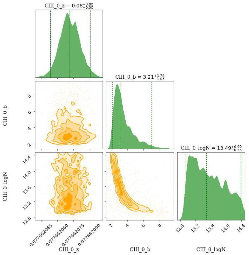
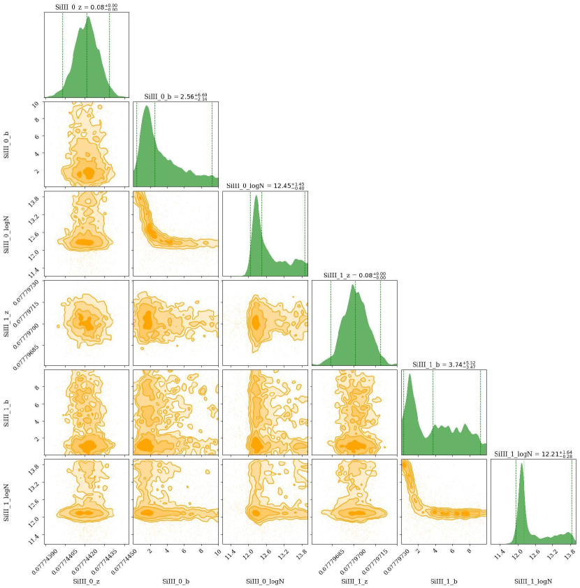
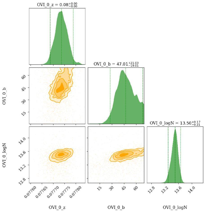
A.2 Posterior distributions for the absorber properties
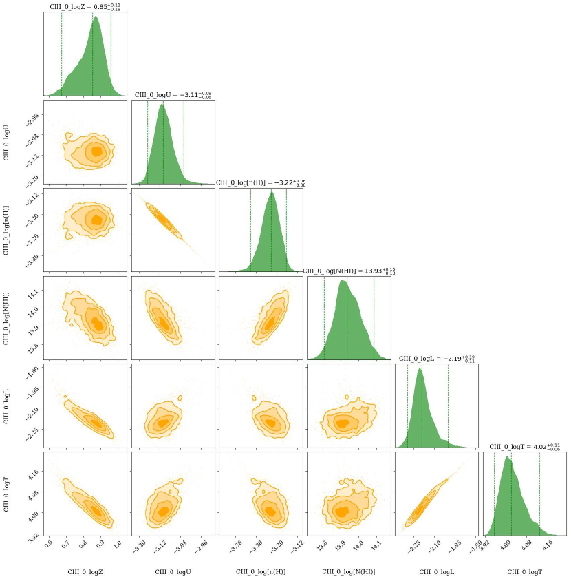
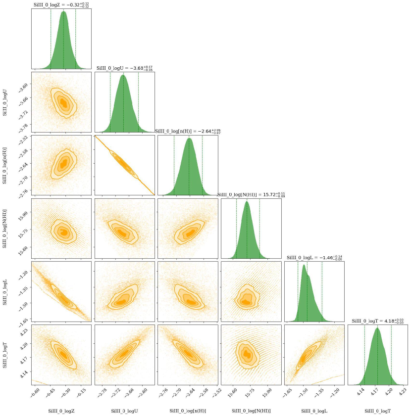
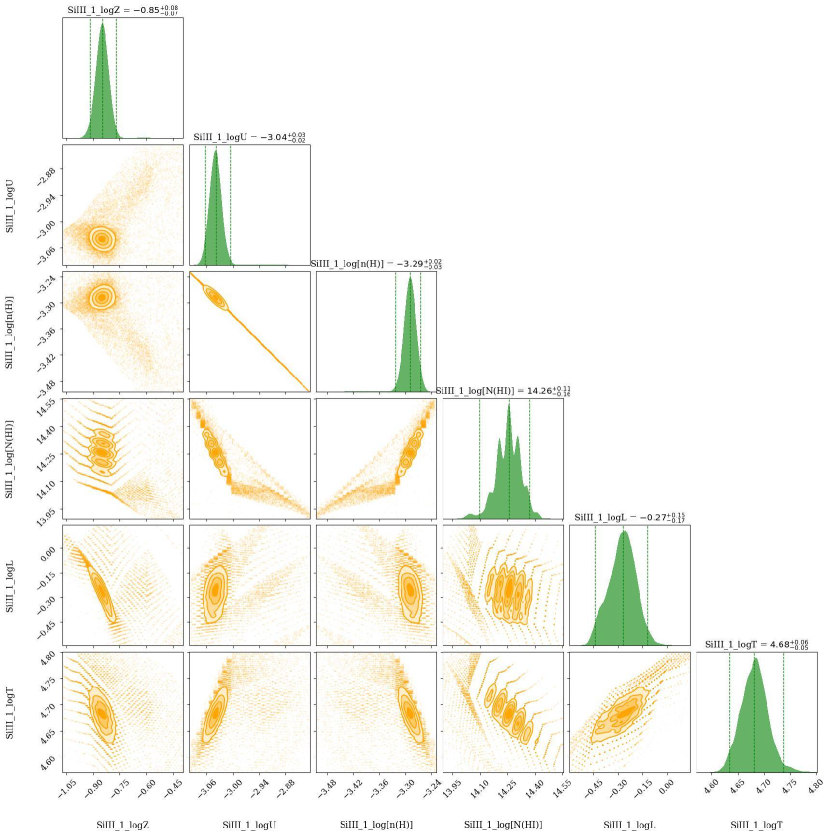
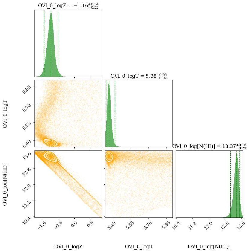
Appendix B Plots for PHL1811 0.08094 absorber
B.1 Posterior distributions for the Voigt Profile fit parameters
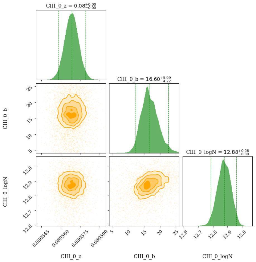
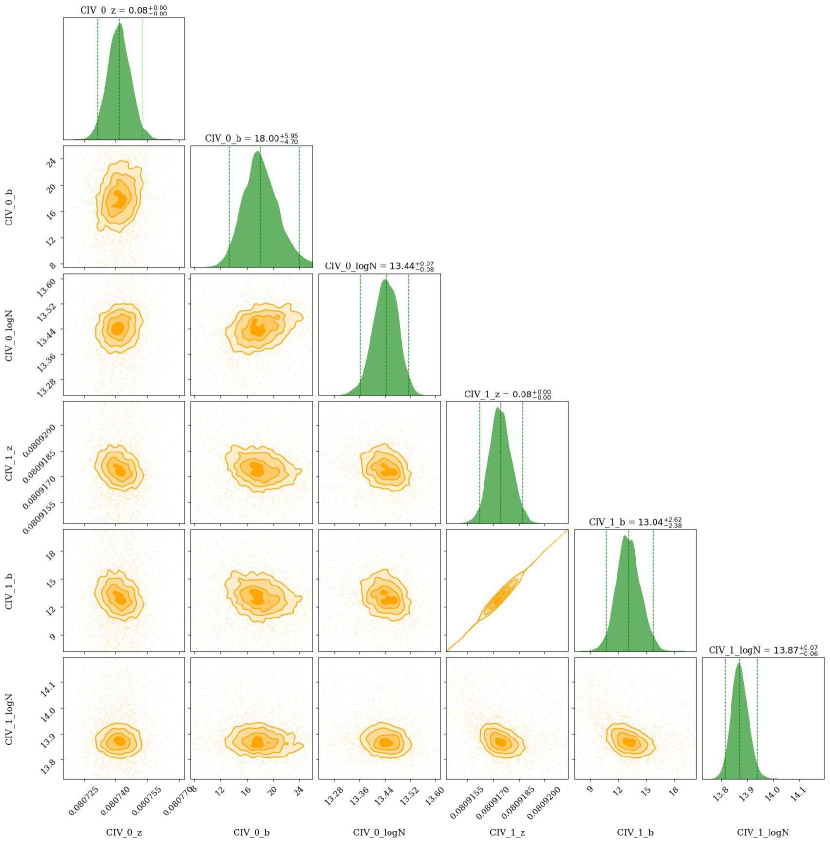
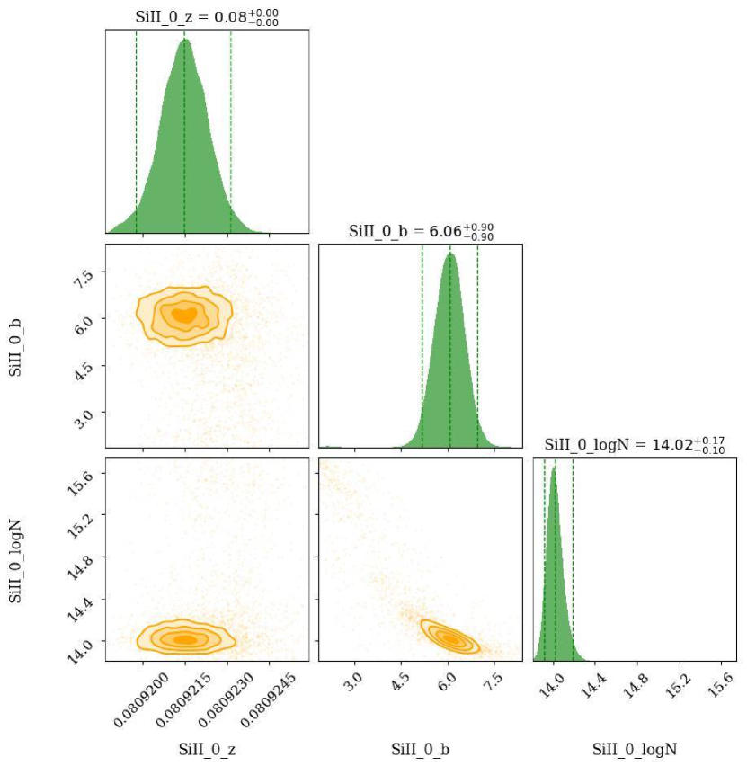
B.2 Posterior distributions for the absorber properties
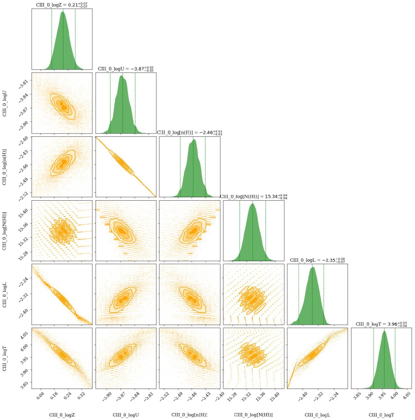
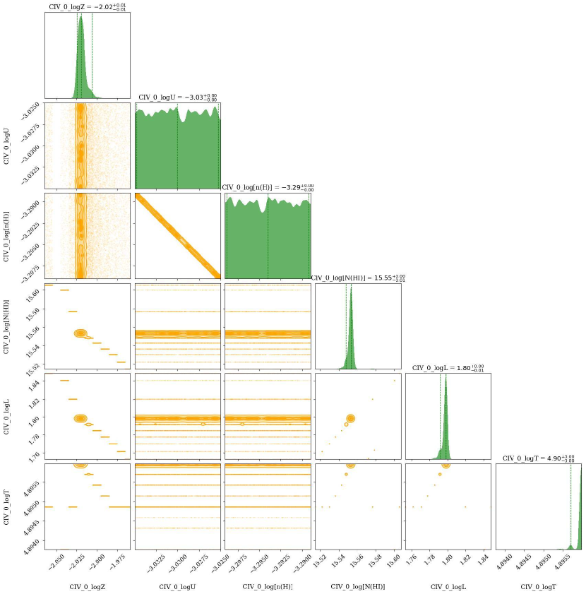
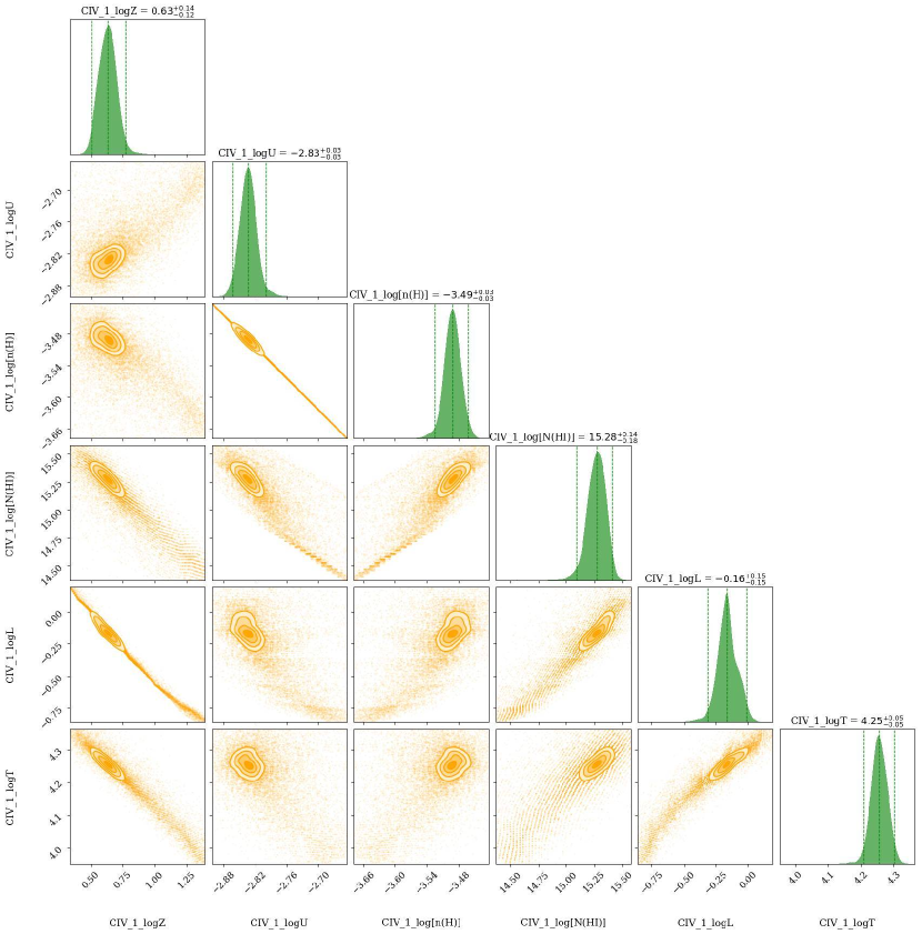
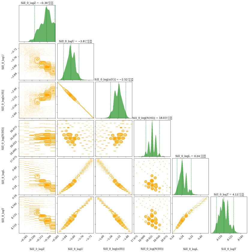
Appendix C Plots for PG1116+215 0.13849 absorber
C.1 Posterior distributions for the Voigt Profile fit parameters
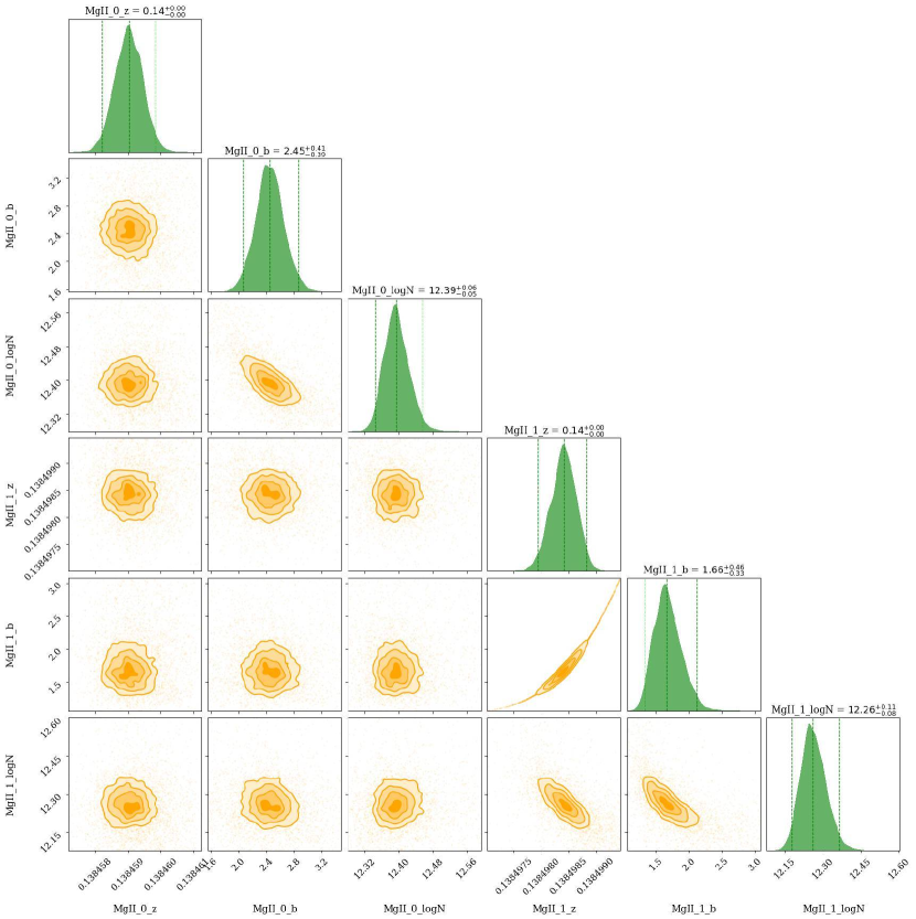
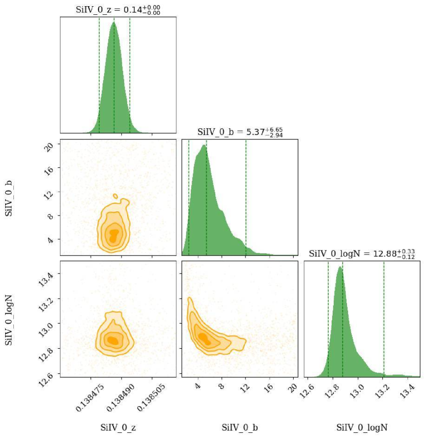
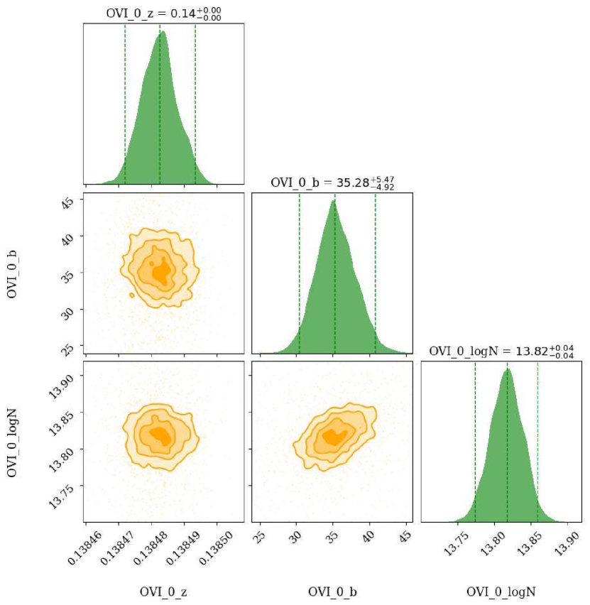
C.2 Posterior distributions for the absorber properties
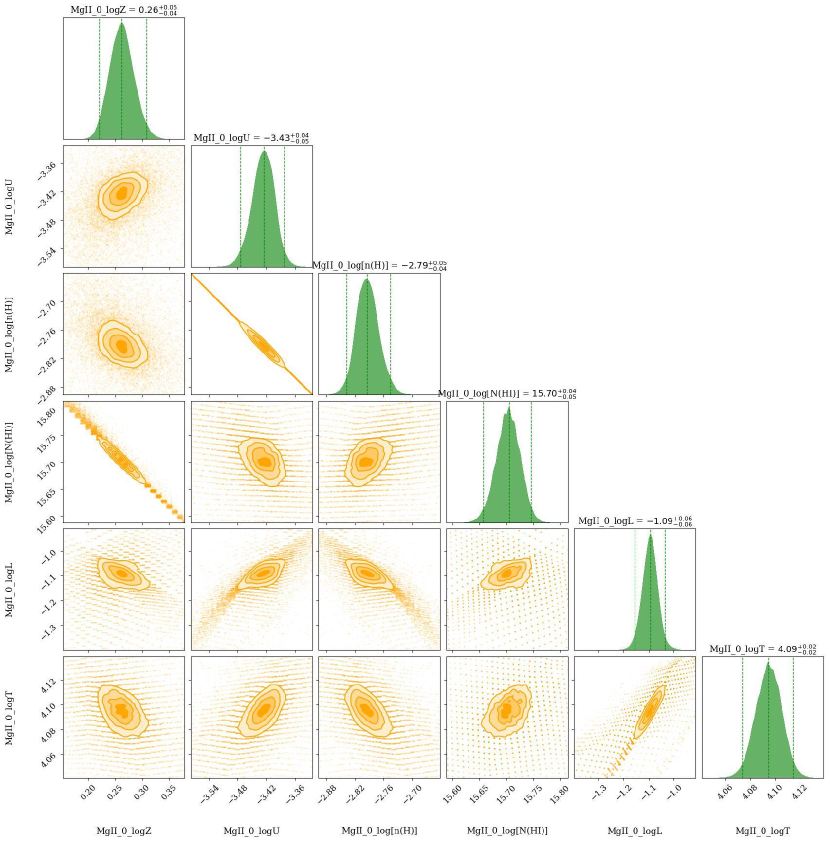
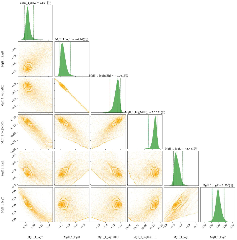
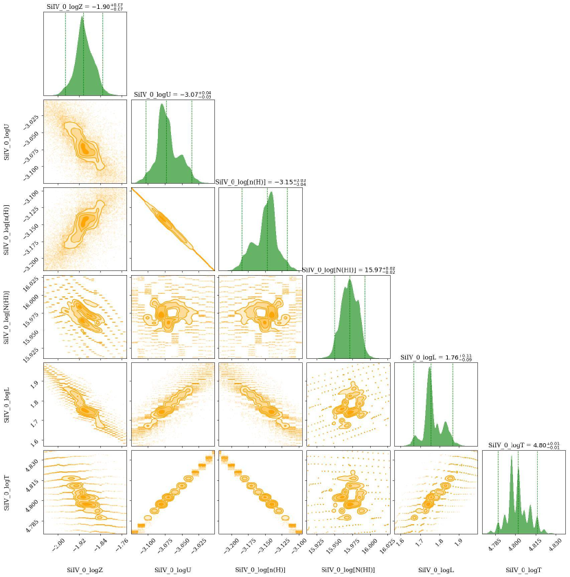
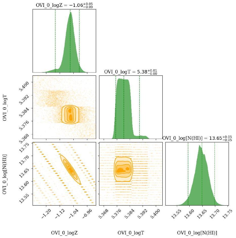
Appendix D Plots for HE0153-4520 0.22596 absorber
D.1 Posterior distributions for the Voigt Profile fit parameters
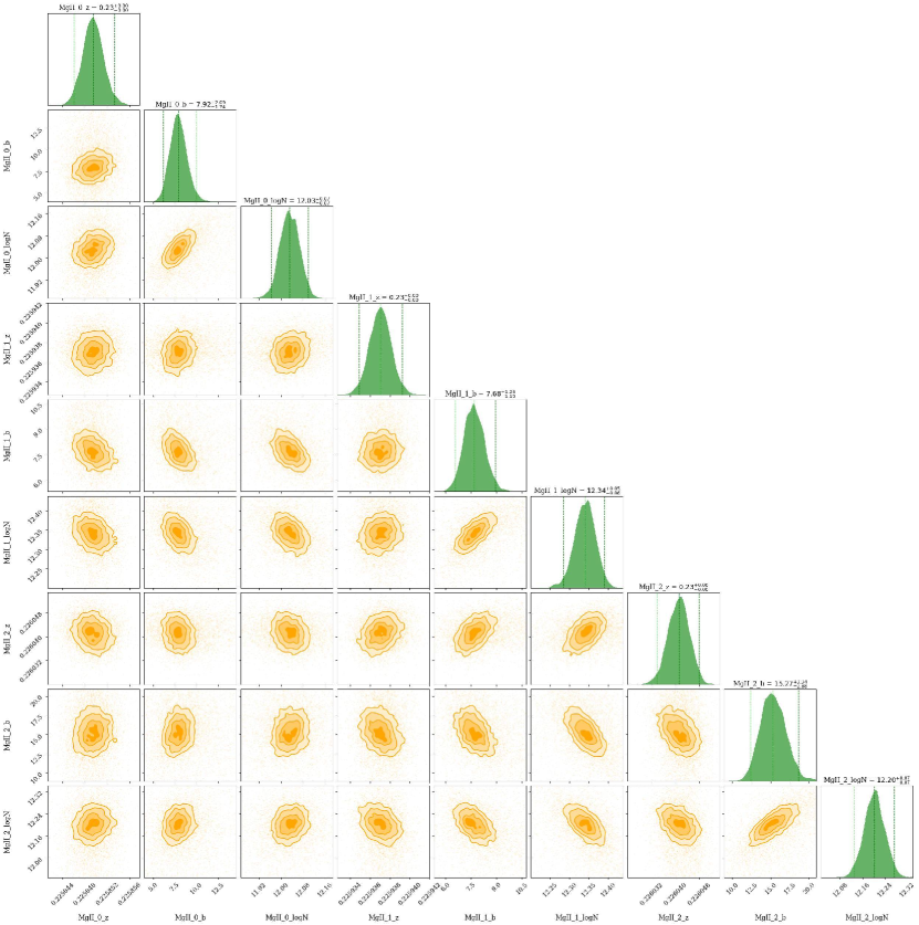
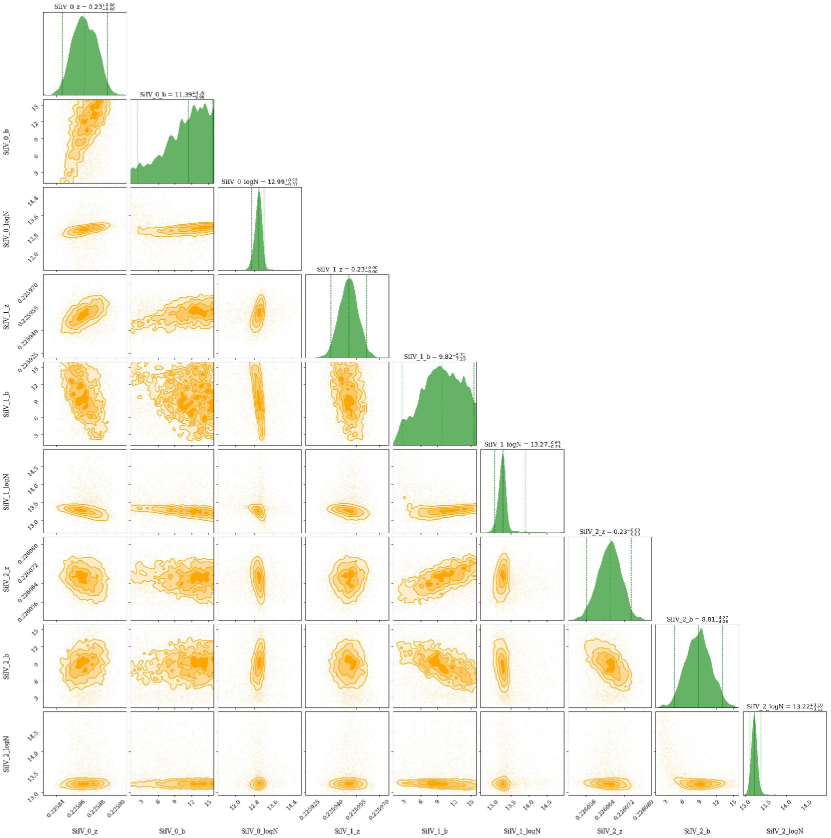
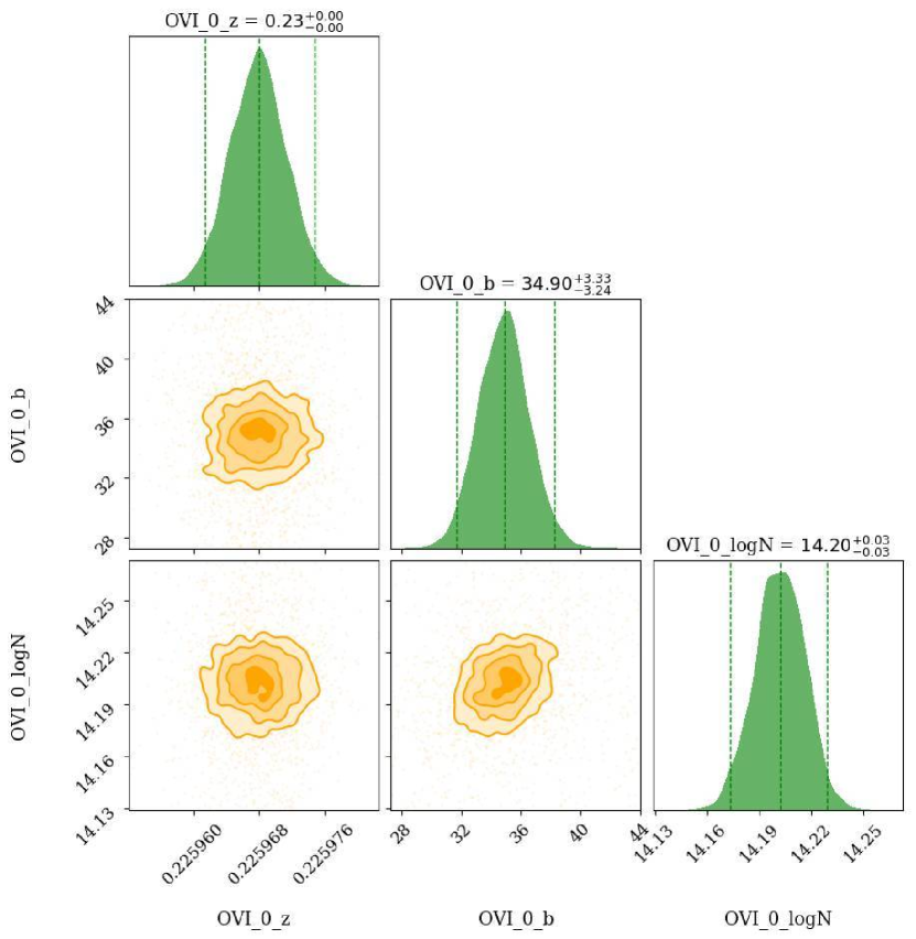
D.2 Posterior distributions for the absorber properties