Cluster algebras and skein algebras for surfaces
Abstract.
We consider two algebras of curves associated to an oriented surface of finite type – the cluster algebra from combinatorial algebra, and the skein algebra from quantum topology. We focus on generalizations of cluster algebras and generalizations of skein algebras that include arcs whose endpoints are marked points on the boundary or in the interior of the surface. We show that the generalizations are closely related by maps that can be explicitly defined, and we explore the structural implications, including (non-)finite generation. We also discuss open questions about the algebraic structure of the algebras.
1. Introduction
Let be an oriented surface with a finite set of marked points, which we distinguish as boundary marked points or interior punctures. The main goals of this paper are to review and clarify relationships between several generalizations of the cluster algebra and the skein algebra of , and to explore the structural implications of this relationship.
The cluster algebra of a surface are a large class of cluster algebras that are particularly well-studied (See [Wil14] for an excellent survey). Cluster algebras are commutative algebras whose generators (cluster variables) and relations (cluster seeds) satisfy mutation properties determined by certain types of combinatorial data [FZ02]. In the case of the cluster algebra of a surface with boundary marked points, the generators correspond to edges of an ideal triangulation, and mutation encodes the combinatorial changes seen when a diagonal edge of the triangulation is flipped [GSV05, FG06]. The definition was motivated by the similarity between the mutation formulas for cluster algebras and the Ptolemy relation for lengths of edges seen in Teichmüller theory, especially as in the work of Penner [Pen87, Pen12]. In the presence of interior marked points, one can also define the cluster algebra, but one needs to combinatorially extend the definition of a triangulation and the edge flip move [FST08, FT18].
The cluster algebra for a surface has been found to be closely related to the Kauffman bracket skein algebra from quantum topology. The skein algebra was introduced in [Prz91, Tur91] as a generalization of the Jones polynomial [Jon85, Kau87] and appears prominently in the associated topological quantum field theory [BHMV95]. The skein algebra is generated by framed loops in modulo the Kauffman bracket skein relations, and it is non-commutative except for a few small surfaces and except when . The skein algebra holds a special place in quantum topology due to its connections to hyperbolic geometry and algebraic geometry. In particular, it is a deformation quantization of the -character variety of the surface [Bul97, PS00, Tur91], which contains the Teichmüller space of .
Because of the common connection to Teichmüller theory, it is natural to expect that there is some compatibility between the cluster algebra and the skein algebra . Actually, because the cluster algebra is generated by edges of an ideal triangulation, a little thought shows that the compatibility should exist with versions of the skein algebra that include arcs between marked points on . One such generalization appeared in work of Roger and Yang [RY14], who wanted to identify their skein algebra as a deformation quantization of Penner’s decorated Teichmüller space for a punctured surface [Pen87, Pen12]. At around the same time, Muller [Mul16] defined a different skein algebra, coming from a quantum cluster algebra for a surface of boundary marked points. Since then, these definitions have been combined and extended to include decorations of (called states) on the boundary marked points [Lê18, BKL24]. We aim to make a precise statement about their relationship with each other and with cluster algebras here.
We remark that similar compatibility results have been proved previously, with different levels of generality and different methods [Mul16, MQ23, MW24]. However, clear statements about the compatibility of the cluster algebra and skein algebra have been missing so far. The known compatibility results have treated only special cases (such as surfaces with only boundary marked points, or only with interior punctures) and only with certain variations. A goal of this paper is to provide general statements that incorporate what is known so far, both by providing references and by explaining how to extend existing proofs.
We begin with definitions of the various generalizations of the skein algebra that include arcs in Section 2. Our primary interest is in the Muller-Roger-Yang generalized skein algebra from [BKL24]. We also discuss the Lê-Roger-Yang generalized skein algebra , which includes states at the boundary marked points. In Section 4, we prove a striking common property, that the skein algebras are finitely generated. In contrast, as we discuss in Section 6.2, the cluster algebra is not always finitely generated.
Theorem A.
The generalized skein algebras and are finitely generated.
It was shown that the original skein algebra was finitely generated in [Bul99], and the proof was extended in for specific cases [Mul16, BPKW16, MW24]. Our proof here applies to the most general case. It immediately follows that some variations of generalized skein algebras are also finitely generated (Corollary 4.2 and 4.5).
In Section 5, we define the cluster algebra for surfaces with both boundary marked points and interior punctures, as well its associated upper cluster algebra . We prove the compatibility of the cluster algebras and skein algebras in Section 6. To do so, we make two modifications. First, observe that the set of boundary edges form a multiplicative subset, and so we may define a localization . Then we set to obtain a commutative skein algebra , and we show that it contains a copy of the cluster algebra. Secondly, we define a certain subalgebra of that is generated by tagged arcs and loops; see Section 6 for the definition. We show that it is contained inside the upper cluster algebra .
Theorem B.
Let be a triangulable marked surface.
-
(1)
There is an inclusion .
-
(2)
There is a subalgebra of (that is generated by tagged arcs and loops) so that there are inclusions
We remark that the second part of Theorem B also appears in [MQ23, Proposition 3.7]. However, at least to the authors, the extension from an unpunctured surface case [Mul16] to punctured surfaces needs some verification. This is because there are no tagged arcs in , but there are vertex classes. We give some brief outline of the argument and references to relevant literature in Section 6.
Due to limited scope and time, the authors decided to restrict discussion here to the generalized skein algebras and , and their variations. The research on the ordinary skein algebra is both long and rich. The results for the obviously inspired the theorems presented in this paper, as well as the open questions from Section 7. Unfortunately, a full discussion and bibliography are outside the scope of our paper. We encourage interested readers to check the references, e.g. [LY21, PBIMW24].
Acknowledgements
We thank the organizers of the special sessions on Knots, Skein Modules, and Categorification at the Joint Mathematical Meetings and Skein Modules in Low Dimensional Topology at a AMS sectional meeting in 2024 for their invitation. HK was supported by JSPS KAKENHI Grant Number JP23K12976. HW was partially supported by DMS-2305414 from the US National Science Foundation.
2. Skein algebras
Let be a compact oriented surface with possibly nonempty boundary , and be a finite set of points of . The pair is called a marked surface. From now on, if there is no chance of confusion, a surface is always a marked surface. We set and call it by the set of boundary marked points. The complement is called the set of interior punctures. Depending on how to treat the arc classes meeting , we use two different types of tangles.
Definition 2.1.
A one-dimensional compact submanifold of equipped with a framing is called a -tangle if
-
(1)
;
-
(2)
.
A -tangle is a one-dimensional compact submanifold with a framing such that
-
(1)
;
-
(2)
for each boundary component of , all points of have different heights;
-
(3)
.
If is a manifold without boundary, both a -tangle and a -tangle are disjoint unions of framed loops on .
Here, we define two generalized skein algebras. For each interior puncture , we assign a formal variable . We fix the Laurent polynomial ring as the coefficient ring. It commutes with all other elements that we will introduce from now on. We also fix .
Definition 2.2 (Muller-Roger-Yang skein algebra ).
The Muller-Roger-Yang skein algebra of a marked surface is a -algebra generated by isotopy classes of -tangles in , modulo the following generalized skein relations:
The multiplication is defined as the stacking of -tangles.
The second generalized skein algebra is based on -tangles and extra states. A state of a -tangle is a map . A stated -tangle is a pair . If there is no confusion, we denote it by .
Definition 2.3 (Lê-Roger-Yang skein algebra ).
The Lê-Roger-Yang skein algebra of a marked surface is a -algebra generated by isotopy classes of stated -tangles in , modulo the relations (A)–(D) and the following extra skein relations:
The multiplication is defined as the stacking of -tangles.
Remark 2.4.
The ordinary Kauffman bracket skein algebra is defined as the algebra generated by isotopy classes of loops in modulo skein relations (A) and (B) [Prz91, Tur91]. The definitions of and follow [BKL24], which combined generalizations of the skein algebra from recent papers including [RY14, Mul16, Lê18, CL22]. If is a surface without any boundary, both and are specialized to the Roger-Yang generalized skein algebra [RY14]. If does not have any interior puncture, is Muller’s skein algebra in [Mul16], and is the stated skein algebra in [Lê18].
We will also consider several variations of and that have appeared in the literature. First, there are the subalgebras generated by tangles that avoid interior punctures. Let be the subalgebra of generated by all -tangles that do not intersect any interior punctures. Similarly, is the subalgebra of generated by all -tangles not meeting interior punctures. Note that relation (C) holds in and .
The next variations drop relation (C). Let (resp. ) be a -algebra generated by all -tangles (-tangles) that do not meet any interior punctures modulo the relataions (A), (B), (D), (E), and (F) (resp. (A), (B), (D), (E’), and (F’)). Then we have morphisms
| (1) |
and
| (2) |
The first map is an epimorphism and is a monomorphism.
The last variation we consider involves a quotient of the stated skein algebras. For each boundary marked point , a -tangle in Figure 1 around is called a bad arc.

Definition 2.5 ([CL22]).
The reduced LRY generalized skein algebra is the quotient of by the two-sided ideal generated by bad arc classes. Let be the quotient map.
We may define similar quotients (resp. ) of (resp. ) by the bad arc classes. We will retain the same notation for the quotient map.
3. Compatibility between skein algebras
In Section 2, we introduced many variations of the skein algebra. From the algebraic perspective, they are not altogether ‘different’ skein algebras, and in this section, we will give a precise relationship between them. Our goal will be to justify the following commutative diagram.
| (3) |
From their definitions, we already have the maps , , and in the diagram. The morphisms and are epimorphisms, and is a monomorphism. We now define the morphisms and .
The homomorphism
| (4) |
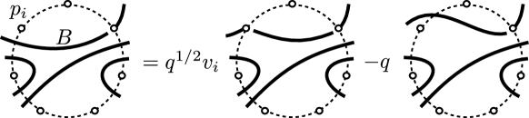
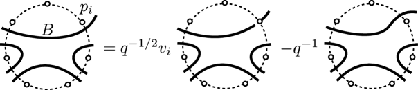
comes from the ‘moving trick.’ Recall that is generated by -tangles, which are one-dimensional submanifolds embedded in . So for each , the heights at the ends are all distinct. For each , we may draw a local diagram around so that all arcs ending at are not tangent to each other, as the diagram on the left in Figure 2. Then, by sliding the ends to the right component of , we obtain a -tangle. For each end , we assign a positive state. Using the skein relations in Definition 2.2, one may check that this is a well-defined map and indeed an algebra homomorphism.
The map is an identity around the interior punctures. Thus, by the same argument, we have similar homomorphisms
| (5) |
We will use the same letter to denote the moving trick homomorphism, to avoid introducing too many notations. Because of the existence of negative states, unless , is not surjective.
We next define the map . Let be the multiplicative subset of generated by boundary arc classes, which are connected -tangles (hence a single arc) joining two boundary marked points on the same connected component of and isotopic to the boundary edge connecting two adjacent marked points on . Since any boundary arc class is -commutative with any -tangles, satisfies the Ore condition [MR01, Section 2.1], hence we may define the Ore localization .
Proposition 3.1.
For any surface , there is an isomorphism
| (6) |
from the localized MRY skein algebra to the reduced LRY skein algebra.
Proof.
We already have a homomorphism
| (7) |
For the algebras appear here, we have explicit -module bases, consisting of tangles without any intersection [BKL24, Theorem 3.6, Theorem 3.11, Proposition 6.2]. By checking that the basis of maps to a subset of the basis of , we may conclude that is a monomorphism.
For any boundary arc class and its image , the same curve with negative states is the multiplicative inverse, so [CL22, Proposition 7.4]. By the universal property of the localization, we obtain a localized homomorphism . Since the original map is injective, so is the localized .
To show the surjectivity of , it is sufficient to show that any arc with negative state is in . Deforming near a boundary marked point and applying the relation (E’) in Definition 2.3, we obtain the following relation.
The first equality is from the skein relation and the second one is from the bad arc relation. The last diagram is in . ∎
4. Finite generation of skein algebra
In this section, we prove that the skein algebras we consider are always finitely generated. In a way, this is rather surprising— as we will see later, the skein algebra contains a copy of a cluster algebra, but in many cases the cluster algebra is not finitely generated. Here we give a skein theoretic proof, extending [Bul99] and [BKWP16], where the finite generation of and were shown. Alternatively, one may prove the finite generation via quantum trace, as done in [BKL24] for .
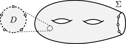
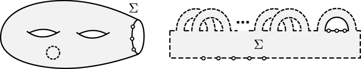
Our strategy is based on the following observation. For a marked surface , the interior punctures in can be drawn on the boundary of a small circular disk on (Figure 3). Then we may understand as a union of a small open neighborhood of and the outside of , that is, . The latter is a surface without interior puncture – now all marked points are on the boundary. We show that is generated by the arc classes in and the curve classes whose supports are in . The former has an explicit finite set of generators [ACDHM21, Section 5]. For the latter, we may employ an extension of the algorithm in [Bul99].
Our discussion will be focused on simple curves, which are curves without any intersections in its diagram. Skein relations (A) and (D) imply that the -algebra is generated by simple curves.
For a simple curve , let be the number of connected components of . We may extend the definition to curves in the isotopy class of , by taking as the minimum of the possible numbers of connected components. The geometric intersection number of and is , and if does not meet .
We may assume that are arranged counterclockwise with respect to the center of . Let be the straight line segment connecting and .
Lemma 4.1.
Let be a simple curve that intersects , so . Then is generated by -subalgebra generated by skeins which do not intersect and .
Proof.
Suppose that has one component with nontrivial intersections with . Let be one of the connected components of such that one of two components of does not have any other components of .
There are two possibilities. If one endpoint of is one of the interior punctures, then as in Figure 4, can be described as a combination of two simple curves and one . Note that and either have smaller intersection number , or the component of without other components of has strictly smaller number of interior punctures. When , the intersection number strictly decreases, too. Thus, after finitely many steps, we may describe in terms of curves with , and .
If none of the endpoints of is not an interior puncture, applying one puncture-skein relation, we may describe as a curve in the previous paragraph and another curve with smaller number of interior punctures on one of the components in (Figure 5). Therefore, after applying the relation finite times, we obtain the conclusion. ∎
Now, it is sufficient to show that any skeins whose supports are in is finitely generated. For this purpose, by stretching the boundary of , we may draw as in the right figure in Figure 6. This diagram is obtained by attaching several handles on a rectangular strip, and all marked points are on the strip itself, not on attached handles. In particular, there is no marked points on the handles. The long dashed boundary is , and the original boundary of is drawn on the top row.
Suppose that is a simple connected curve whose support is in . We fix an arbitrary orientation on . Assume that there is a handle on such that traverses multiple times in the same direction. See the left figure in Figure 7. Then an ordinary skein relation can be applied to rewrite the curve in terms of curves that traverse strictly fewer times (Figure 7). Note that the rightmost diagram is a product of two disjoint curve classes, and each of these curves traverses strictly fewer times than the original diagram on the left hand side of the equation. By applying this argument in pairs, we may assume that travels each handle at most twice, and if so, it travels exactly twice in the opposite direction.

Next, suppose that there is a handle where travels twice, in opposite directions (top left of Figure 8). We may employ the ordinary skein relations three times, to write it as a combination of curves which traverse the handle at most once. See Figure 8.
Note that Bullock applied the above algorithm only to loops in [Bul99]. However, the argument works equally well for arc classes. This is because the resolutions in Figures 7 and 8 do not change the part of the arc outside (on the parts of the arc diagram that are dotted in the figures).

In summary, any simple curve can be generated by simple curves that traverse each handle at most once. These curves can be described by choosing the finite sequence of traveling handles in the case of loops and by choosing the initial/terminal marked points and the sequence of traveling handles in the case of arcs. (We do not claim that all sequences of handles will give simple curves and arcs – they may induce self-intersections.) Thus, there are only finitely many possibilities. As a result, we obtain the proof of Theorem A.
Corollary 4.2.
The skein algebras and are finitely generated.
Proof.
The skein algebra can be generated by 1) the image of a generating set of by , and 2) the same set of curves with different states. The algebra is generated by finitely many loops and arcs, and for each arc connecting boundary marked points, there are only finitely many ways to impose the states. Therefore, is finitely generated, too. A homomorphic image of a finitely generated algebra is also finitely generated, so the same thing holds for . ∎
Remark 4.3.
One can show is finitely generated in another way, directly from from Proposition 3.1. Since is an Ore localization of a finitely generated algebra by a finitely generated multiplicative subset , it is also finitely generated.
Remark 4.4.
The finite generating set from the proof of Theorem A is not guaranteed to be minimal. Note that the non-boundary handles appear as pairs. Suppose that travels both handles (say and ) in a pair. Bullock proved that can be generated by curves that passes immediately traveling after [Bul99]. A minimal set of generators is not known, and is closely related to the computation of an explicit presentation of . See Section 7.1.
If we remove each interior puncture by a new boundary component without a marked point, the same proof of Theorem A works for . Then we also obtain that is finitely generated in the same way. Any homomorphic image of a finitely generated algebra is also finitely generated, so we obtain the following corollary.
Corollary 4.5.
The skein algebras , , , , , and are all finitely generated.
Remark 4.6.
For any oriented surface with interior punctures, we may draw the punctures on a small circular disk as we did in the proof of Theorem A. Then for a small open neighborhood of , there is a natural morphism
| (8) |
In other words, admits an -algebra structure. Note that is homeomorphic to , the -punctured . Its skein algebra was calculated in [ACDHM21, Section 5].
5. Cluster algebra of surface
We next consider the cluster algebra coming from the curves in a triangulable oriented surface . In this section, we give a brief definition of . A more detailed description and further properties of can be found in [FST08, FT18]. In Section 6, we will explain its relationship with the skein algebra.
5.1. Informal description
Let be a surface that admits an ideal triangulation , with the set of vertices . Here an ideal triangulation always contains all boundary arcs. Let be the set of edges in . The cluster algebra is defined as some subalgebra of the field of fractions generated by edges in subject to geometrically motivated relations. Because the formal definition will require some additional structure on the edges, it may seem overly technical at first. We thus start with an intuitive description to give the flavor of the construction and worry about the technical details later.
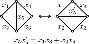
The basic construction of the cluster algebra is based on the following idea. For a given triangulation and a choice of an internal diagonal edge of a quadrilateral, we may flip the diagonal edge in the triangulation to the other diagonal edge of the quadrilateral. This move produces a new triangulation where all edges are the same as in except that is replaced by a flipped edge (Figure 9).
In the cluster algebra, we relate the edges and using the Ptolemy relation, which comes from the geometry of relating the lengths of the edges of the quadrilateral with its diagonals. More specifically, suppose that the quadrilateral has edges , , , and , and flipping the diagonal of the quadrilateral gives a new diagonal , as in Figure 9. In this case, the Ptolemy relation between and is defined to be . Observe that the product is a ‘binomial’ with respect to the quadrilateral edges , , , and , and that is a rational function with respect to edges in . As a result, we can think of the edges in the new triangulation as belonging in the field of fractions of the edges of the original triangulation . Moreover, the combinatorial changes between the edges of and can also be encoded algebraically by way of mutation of the adjacency matrices, and we will provide these equations later.
The cluster algebra we seek to define is very ‘close’ to the subalgebra of generated by all the edges of all possible triangulations subject to the Ptolemy relation and mutation of adjacency matrices. Importantly, the resulting can be regarded as an algebra of all arcs on . Recall that, any embedded arc between two vertices belongs to some ideal triangulation on . Moreover, any two ideal triangulations are connected by finitely many flips. In the algebra, each time we flip an edge in , we obtain a new triangulation with one new edge that is related to the old ones by the Ptolemy relation. Although the number of generators of the cluster algebra is a priori infinite, it turns out that any arc can be written in terms of the edges of the original triangulation . The upshot is that we can think of any embedded arc of as belonging in , and the cluster algebra is an algebra of curves.
However, there are some technical issues that arise when aligning this intuitive construction of with the standard definition of cluster algebras. In particular, all elements of a cluster algebra should be flippable. However, boundary edges are never diagonals of any quadrilaterial and hence never flippable. This can be accounted for by using a version of the cluster algebra where the boundary edges are frozen variables. In cluster algebra literature, it is common to include the multiplicative inverses of the frozen variables, so we will take the same convention.
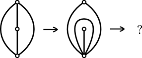
A more serious issue comes up when there are interior punctures. In particular, consider the part of an ideal triangulation in Figure 10. One may flip the top interior edge, to get a new triangulation with a self-folded triangle. However, now the bottom edge connecting the two bottom punctures (inside of the self-folded triangle) is no longer a diagonal of a quadrilateral and thus cannot be flipped.
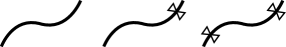
To rectify this issue, in [FST08], Fomin, Shapiro, and Thurston introduced the additional structure of tagged arcs to account for the combinatorics of self-folded triangles. A tagged arc is a topological arc where each end can be decorated by one of two taggings, plain or notched. The notched end is denoted by drawing a small bowtie, and the plain end is unmarked. The three possible types of tagged arcs are illustrated in Figure 11.
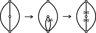
Triangulations can then be generalized to include tagged arcs, and every tagged arc can now be flipped as in Figure 12. This new diagrammatic procedure for tagged arcs is called a tagged flip, and its combinatorics are designed to match that of ordinary flips along diagonals of quadrilaterals. For the details, see [FST08, Section 7], [MW24, Section 3].
We emphasize that a tagged arc can have a notched end only at an interior puncture. Boundary arcs and arcs connecting boundary marked points cannot have any tags. So, in the absence of interior punctures, the additional structure of tagging is not needed at all to define the cluster algebra of the surface.
5.2. Formal definition
In this section, we give a quick reminder of the construction of the cluster algebra of surfaces. For the general theory of cluster algebras, [Wil14] is an excellent introduction. For the details of the tagged arcs and tagged triangulations, see [FST08, Section 7].
Let be a tagged ideal triangulation on . In other words, is a maximal collection of pairwise compatible tagged arcs.111Here, two tagged arcs are said to be compatible if their untagged versions are disjoint except at and their taggings satisfy a technical condition if they share an endpoint: if the two arcs are not isotopic and meet at an endpoint, then their taggings at that end must be identical; and if the two arcs are isotopic and meet at an endpoint, then at least one one of the two ends must be identical. Let be the set of edges in , and be a fixed index set for edges in . We divide , where is the index set for interior edges and is the index set for boundary edges.
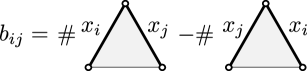
A seed is a collection of data , where is the set of edges in and is an matrix such that its entry is given by Figure 13, that is, a signed counting of the adjacency of two edges and on the triangulation, i.e. and are edges of an ideal triangle. Thus, and is a skew-symmetric matrix. The matrix is called the exchange matrix.
For each choice of , we can construct a new seed in the following way. Observe that there is a unique way to flip to another arc , corresponding to the procedure of Figure 9 or 12. We may thus replace by in to obtain a new tagged triangulation . Let denote the new set of edges in . For edges , . In the cluster algebra, the exchange relation relates the variables and by
| (9) |
The new exchange matrix for is then
| (10) |
The cluster mutation in the -th direction is defined to be the map . One can check that this formal definition captures the combinatorial changes from flipping an edge. One can also check that is an involution, i.e., .
Notice that boundary edges correspond to frozen variables. In particular, cluster mutation is not defined for .
Definition 5.1.
Let be a triangulated surface with an initial seed coming from a fixed triangulation . The cluster algebra is a subalgebra of generated by
| (11) |
for all cluster seeds obtained by taking a finite sequence of cluster mutations.
It is well-known that does not depend on the choice of the initial seed. Thus, it is an invariant of a marked surface .
Example 5.2.
Let be the torus with one interior puncture. We draw the torus using a standard square diagram as in Figure 14. We fix an ideal triangulation with . One may check that its exchange matrix is
| (12) |
Flipping , we obtain a new triangulation as in the right figure in Figure 14. This cluster mutation results in a new seed , where
| (13) |
Remark 5.3.
When is a surface with one interior puncture and without boundary, one can check that no triangulation admits any self-folded triangle as in the second Figure in Figure 10 and any arc is flippable. In particular, tagged arcs are unnecessary to define .
Theorem 5.4 ([FST08, Theorem 7.11]).
Let be a triangulated surface with an initial seed coming from a fixed triangulation . Suppose that is not a once-punctured surface without boundary. Then the cluster algebra is generated by arcs and tagged arcs. If is a once-punctured surface without boundary, or a surface without interior puncture, then is generated by ordinary arc classes.
Remark 5.5.
In this paper, we focus on the cluster algebra of a triangulated surface . However, the cluster algebra can be defined for more general situation. Suppose that we have a finite list of variables , a decomposition of the index set (Note that in the case of , and .) and a skew-symmetric integral matrix . Then is defined as subalgebra of that is generated by
| (14) |
where is a cluster seed obtained by taking a finite sequence of cluster mutations.
5.3. Upper cluster algebra
For each cluster algebra , one may define another algebra, the so-called upper cluster algebra , which seems to be more natural from the algebraic geometry viewpoint and behave better algebraically [BFZ05]. In this section, we review the definition of the upper cluster algebra in the context of a cluster algebra of a surface .
Let be a triangulated marked surface and be the cluster algebra associated to . Recall that any two cluster seeds and are connected by a finite sequence of cluster mutations. So by applying the exchange relation (9) finitely many times, we may algebraically relate with . More specifically, if we denote and , any can be written as a rational function with respect to . One can say more about the type of rational functions obtained in this way.
Theorem 5.6 (Laurent phenomenon [FZ02, Theorem 3.1]).
For any two cluster seeds and for ,
| (15) |
In other words, is a Laurent polynomial with respect to any cluster seed.
Definition 5.7.
Consider a cluster algebra . The upper cluster algebra is defined as the set of all elements in that can be written as a Laurent polynomial with respect to arbitrary seeds. In other words,
| (16) |
6. Compatibility between skein algebra and cluster algebra
We now prove Theorem B, starting with a review of relevant definitions.
6.1. Cluster algebra in skein algebra
Fix a tagged triangulation , or equivalently, a cluster seed of where each corresponds to a tagged arc. Note that if a tagged arc ends at an interior puncture , then that end of can be decorated in one of two ways: plain or notched. See Figure 11. For each tagged arc , let be its underlying topological arc after forgetting its tags. We can then understand as an element of .
Consider the subalgebra .
Definition 6.1.
Fix a cluster seed . Suppose that is a tagged arc connecting and (not necessarily distinct). We set
| (17) |
By extend it using the universal property of the polynomial ring, we obtain an algebra homomorphism
| (18) |
Note that any boundary edge is not tagged. Thus, simply maps to and gives a well-defined element in .
The slogan for is: “A tag is a vertex class.” Whenever one has a notch on a tagged arc, replace the notched end by a vertex class.
Proof of Part (1) of Theorem B.
For each cluster seed, we have a well-defined homomorphism in (18). To prove the statement, we first show that these homomorphisms are compatible: If and are connected by a single flip, then for any element in
| (19) |
the image of and coincide. Thus, we may ‘glue’ the two homomorphisms to get .
One may describe all possible tagged flips and for each one, calculating the mutation explicitly. It was done in [MW24, Proposition 4.3] using puzzle pieces. The paper covered only surfaces without boundary, but note that we do not flip any boundary edge, so the same list of cases covers all possible cases here, too.
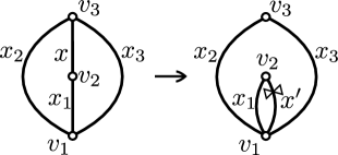
To give a flavor of the type of computation, we now reproduce the proof using puzzle pieces for one particular case. Consider the tagged flip described in Figure 15. For this flip, the only nontrivial change is made for , and by the exchange relation (9), we obtain . On the other hand, the puncture-skein relation in Definition 2.2 (after setting ) provides . Therefore,
| (20) |
With similar calculations on other cases, we obtain a well-defined morphism . To finish the proof, we need to show that is a monomorphism.
Fix an ordinary triangulation whose set of edges is . We claim that both and admit a morphism to the Laurent polynomials in ,
For , the Laurent phenomenon of Theorem 5.6 provides an inclusion . We denote the inclusion map by . For , one needs to show that any vertices and loop classes are Laurent polynomials. The computation for the loop classes and general arc classes not necessarily in is well-known in skein theory literature. For instance, see [RY14, Theorem 3.22]. Applying puncture-skein relation, any interior puncture is also a Laurent polynomial in . For instance, in Figure 15, .
Thus, we have the following commutative diagram of commutative algebras:
| (21) |
Since is injective, is injective, too. ∎
Remark 6.2.
Note that the above proof does not claim that is also injective. We believe it has to be shown separately. If any edge is not a zero divisor, then the localization map is injective. But how do we know that the multiplication of an arc on is injective? One way to show it is using dimension theory from algebraic geometry. Apply an algebraic ring extension of in and construct an epimorphism . Since is an epimorphism from an integral domain with the same dimension, its kernel is trivial [MW24, Theorem 5.2]. Thus, and the latter is an integral domain, and any nonzero element is not a zero divisor.
Observe that the above proof tells us that any loop class in is a Laurent polynomial with respect to any fixed ordinary triangulation. The same Laurent polynomial formula also applies to tagged triangulation [MSW11, Proposition 3.15]. It thus follows that all loop classes are in . However, even though each vertex class is a Laurent polynomial with respect to an ordinary triangulation, it is not with respect to a tagged triangulation. Therefore, it does not belong to .
Definition 6.3.
Let be a subalgebra of generated by:
-
(1)
loop classes;
-
(2)
all arc classes;
-
(3)
all formal inverses of boundary arc classes;
-
(4)
if is an arc class connecting two (non-necessarily distinct) interior punctures and ; , , and ;
-
(5)
if is an arc class connecting an interior puncture and a boundary marked point, .
Proof of Part (2) of Theorem B.
When , we may define in a simpler way: It is a subalgebra of generated by the image of and the loop classes. Since is generated by and the loop classes, any element in is in . ∎
We also obtain the following structural results:
Proposition 6.4.
Let be a marked surface.
-
(1)
is finitely generated.
-
(2)
is an integral domain.
6.2. Applications of Compatibility
There are a few applications to the structure of .
In general, it has been observed that the ordinary cluster algebra may behave badly, but its upper cluster algebra has better structure. For instance, in many cases, is a finitely generated algebra, hence it defines an affine irreducible algebraic variety . (However, there are some infinitely generated examples [Spe13, GHK15].) Moreover, is integrally closed [Mul13, Proposition 2.1], so is a normal variety, which means its singularity type is relatively mild (the singular locus is of codimension , etc.). So one may ask if , for a given cluster algebra.
In the case of cluster algebra of surfaces, if there is at least one boundary component, then [Mul13, MSW13, CLS15, MS16]. On the other hand, if is a surface without boundary but with one interior puncture, then [Lad13], which was shown by constructing an explicit element in .
An application of the compatibility between and can be used to show that when [MW24, Section 6]. We summarize the argument here. Using techniques from invariant theory with -coefficients, it was shown that with cannot be generated by finitely many elements [MW24, Theorem C]. By way of contradiction, assume . Since , this would imply that . But is finitely generated (Proposition 6.4), a contradiction.
In the case of , the -punctured sphere, it was a folklore conjecture that is finitely generated. The computation in [ACDHM21] indeed implies that . Therefore, the finite generation of follows. We do not know if or not.
The finite generation problem for itself is an interesting problem. As we mentioned earlier, it was shown that is not finitely generated when [MW24, Section 6]. Note that from Proposition 6.4 and Theorem B, when , we immediately obtain the finite generation of . The previous results and the discussion above show that if the given triangulated surface has boundary or , is finitely generated. Therefore, we have a complete understanding on the finite generation problem for .
Remark 6.5.
The skein algebra and its variations are non-commutative (except for some small surfaces), and one can think of them as ‘quantum’ versions of the commutative . Similarly, one may wonder if we can obtain a ‘quantum’ analogue of . More generally, for a cluster algebra whose exchange matrix is of full-rank, its deformation quantization was studied in [BZ05] and called the quantum cluster algebra. However, if the exchange matrix is not of full-rank, it is not possible to obtain [BZ05, Proposition 3.3]. It is also well-known that the exchange matrix for is not of full-rank if has an interior puncture. Thus, for a surface with an interior puncture, does not provide a desired deformation quantization.
On the other hand, note that can be defined for any oriented surface and it is a quantization of . Therefore, from Theorem B, we may understand as a quantization of .
7. Open questions
In this last section, we leave a few open questions on the structures of cluster algebras and skein algebras of surfaces.
7.1. Algebraic structure of skein algebras
By Theorem A, and its variations are all finitely generated algebras. However, numerous questions remain about its multiplicative structure. For example, a presentation of the skein algebra is currently known only for a few small surfaces.
Question 7.1.
-
(1)
Compute a presentation of .
-
(2)
Find a minimal number of generators of .
To the best of our knowledge, the presentation has been computed for the once-puncture torus [BPKW16] and for the -punctured sphere [ACDHM21]. Note that in these two cases, there is no boundary component, so the localization is not necessary. Even though it is not explicitly stated, the case of a disk with boundary marked points can be obtained from [FZ03, Section 12]. The case of the annulus with one marked point on each boundary component appears in [Lê15].
Recall that is an -punctured open disk. Note that when , the commutative algebra naturally appears in many different contexts, including in classical invariant theory, as the coordinate ring of the Grassmannian, and in tropical geometry. Consult [ACDHM21, Remark 5.2] for additional discussion.
Question 7.2.
Identify for a simple surface with other algebraic structures.
One may investigate other algebraic properties of . It has been known that is a domain [BKL24] as a corollary of an embedding into a quantum torus, and its center has been calculated when is a primitive root of unity of odd order [KMW25]. A similar result was obtained for in [Yu23a] and for in [Kor21]. From its connection to the cluster algebra, it has been conjectured that has a ‘positive basis,’ that is, a -basis whose multiplicative structure constants are all in [Thu14] after we replace with in the ground ring. See related results in [DM21, MQ23].
Question 7.3.
-
(1)
Do the generalized skein algebras each admit a positive basis?
-
(2)
Compute the structure constants and describe them geometrically.
For a partial evidence for , see [Kar24].
7.2. Upper cluster algebra
From Section 6, we have that . Currently, there are no known elements in but not in . This suggests:
Question 7.4.
Is it true that ?
Between and , there is another algebra motivated by mirror symmetry, so-called the mid cluster algebra [GHKK18]. It was shown that [MQ23, Theorem 1.3]. It is not known whether or not and are equal.
Observe that if , Proposition 6.4 implies that is finitely generated.
This compatibility of and seems to be a part of more general phenomenon. One may understand our as the theory with the structure group , in the framework of higher Teichm̈uller theory in [FG06]. For some other structure groups of row rank, there are similar results [IOS23, IY23]. It suggests that for a higher structure group, where the skein theory is not clear, the skein algebra is expected to be ‘defined’ as the upper cluster algebra.
7.3. Representation theory of skein algebra
A natural next step would be to study the representation theory of . There have been some investigations for quantum cluster algebras and localized Muller skein algebras with boundary edges [MNTY24, Kor21, Kor22, KK23]. However, less is known about the representation theory for variations of the skein algebra in the presence of interior punctures, as in the Roger-Yang skein algebra.
Based on techniques adapted from these earlier works, [KMW25, Proposition 5.5] showed that when is an odd primitive root of unity, (hence too) is an almost Azumaya algebra. This means ‘most’ of irreducible representations can be identified with points in an open dense subset . See [KMW25, Section 5] for more details. The open set is called the Azumaya locus of . The center was calculated in [KMW25, Theorem A]. However, we do not yet have an explicit description of the representations of .
Question 7.5.
-
(1)
Describe the Azumaya locus explicitly.
-
(2)
For each point , construct the corresponding finite dimensional irreducible representation of geometrically.
The ordinary skein algebra can be regarded as a quantization of the Teichmüller space of , and its representations are closely related to hyperbolic geometric data of the surface . Similarly, since is based on combinatorial data from the decorated Teichmüller space of by extending the discussion in [RY14, Mul16], it would be interesting to see how the representations of are related to the hyperbolic geometry of as well.
References
- [ACDHM21] F. Azad, Z. Chen, M. Dreyer, R. Horowitz, and H.-B. Moon. Presentations of the Roger-Yang generalized skein algebra. Algebr. Geom. Topol., 21 (2021), no. 6, 3199–3220.
- [BFZ05] A. Berenstein, S. Fomin, and A. Zelevinsky. Cluster algebras. III. Upper bounds and double Bruhat cells. Duke Math. J. 126 (2005), no. 1, 1–52.
- [BZ05] A. Berenstein and A. Zelevinsky. Quantum cluster algebras, Adv. Math. 195 (2005), no. 2, 405–455.
- [BHMV95] C. Blanchet, N. Habegger, G. Masbaum and P. Vogel. Topological quantum field theories derived from the Kauffman bracket, Topology 34 (1995), no. 4, 883–927.
- [BKL24] W. Bloomquist, H. Karuo and T. Lê. Degenerations of skein algebras and quantum traces. to appear in Trans. Amer. Math. Soc. (2024)
- [BKWP16] M. Bobb, S. Kennedy, H. Wong, and D. Peifer. Roger and Yang’s Kauffman bracket arc algebra is finitely generated. J. Knot Theory Ramifications 25 (2016), no. 6, 1650034, 14 pp.
- [BPKW16] M. Bobb, D. Peifer, S. Kennedy, and H. Wong. Presentations of Roger and Yang’s Kauffman bracket arc algebra. Involve 9 (2016), no. 4, 689–698.
- [Bul97] D. Bullock. Rings of SL2(C)-characters and the Kauffman bracket skein module, Comment. Math. Helv. 72 (1997), no. 4, 521–542.
- [Bul99] D. Bullock. A finite set of generators for the Kauffman bracket skein algebra. Math. Z. 231(1) (1999) 91–101.
- [CLS15] I. Canakci, K. Lee, and R. Schiffler. On cluster algebras from unpunctured surfaces with one marked point. Proc. Amer. Math. Soc. Ser. B 2 (2015), 35–49.
- [CL22] F. Costantino and T. Le. Stated skein algebras of surfaces. J. Eur. Math. Soc. (JEMS) 24 (2022), no. 12, 4063–4142.
- [DM21] B. Davison and T. Mandel. Strong positivity for quantum theta bases of quantum cluster algebras. Invent. Math. 226 (2021), no. 3, 725–843.
- [FG06] V. Fock and A. Goncharov. Moduli spaces of local systems and higher Teichmüller theory. Publ. Math. Inst. Hautes Études Sci. No. 103 (2006), 1–211.
- [FST08] S. Fomin, M. Shapiro, and D. Thurston. Cluster algebras and triangulated surfaces. I. Cluster complexes. Acta Math. 201 (2008), no. 1, 83–146.
- [FT18] S. Fomin and D. Thurston. Cluster algebras and triangulated surfaces Part II: Lambda lengths Mem. Amer. Math. Soc. 255 (2018), no. 1223, v+97 pp.
- [FZ02] S. Fomin and A. Zelevinsky. Cluster algebras. I. Foundations. J. Amer. Math. Soc. 15 (2002), no. 2, 497–529.
- [FZ03] S. Fomin and A. Zelevinsky. Cluster algebras II: finite type classification. Invent. Math. 154 (2003) 63–121.
- [GSV05] M. Gekhtman, M. Shapiro, and A. Vainshtein. Cluster algebras and Weil-Petersson forms. Duke Math. J. 127 (2005), no. 2, 291–311.
- [GHK15] M. Gross, P. Hacking, and S. Keel. Birational geometry of cluster algebras. Algebr. Geom. 2 (2015), no. 2, 137–175.
- [GHKK18] M. Gross, P. Hacking, S. Keel, and M. Kontsevich. Canonical bases for cluster algebras. J. Amer. Math. Soc. 31 (2018), no. 2, 497–608.
- [IOS23] T. Ishibashi, H. Oya, and L. Shen. for cluster algebras from moduli spaces of -local systems Adv. Math. 431 (2023), Paper No. 109256, 50 pp.
- [IY23] T. Ishibashi and W. Yuasa. Skein and cluster algebras of unpunctured surfaces for . Math. Z. 303 (2023), no. 3, Paper No. 72, 60 pp.
- [Jon85] V.F.R. Jones. A new polynomial invariant for links via von Neumann algebras. Bull. Amer. Math. Soc. 12 (1985), 103–122.
- [Kar24] H. Karuo. On positivity of Roger-Yang skein algebras. J. Algebra 647 (2024), 312–326.
- [KK23] H. Karuo and J. Korinman. Classification of semi-weight representations of reduced stated skein algebras. arXiv:2303.09433 (2023).
- [KMW25] H. Karuo, H.-B. Moon, and H. Wong. Center of generalized skein algebras. preprint. arXiv:2501.10686.
- [Kau87] L. Kauffman. State models and the Jones polynomial. Topology 26 (1987), no.3, 395–407.
- [Kor21] J. Korinman. Unicity for representations of reduced stated skein algebras. Topology Appl. 293 (2021), Paper No. 107570, 28 pp.
- [Kor22] J. Korinman. Mapping class group representations derived from stated skein algebras. SIGMA Symmetry Integrability Geom. Methods Appl. 18 (2022), Paper No. 064, 35 pp.
- [Lad13] S. Ladkani. On cluster algebras from once punctured closed surfaces. preprint. arXiv:1310:4454.
- [Lê15] T. T. Q. Lê. On Kauffman bracket skein modules at roots of unity. Algebr. Geom. Topol. 15 (2015), no. 2, 1093–1117.
- [Lê18] T. T. Q. Lê. Triangular decomposition of skein algebras. Quantum Topology 9 (2018), 591–632.
- [LY21] T. T. Q. Lê and T. Yu. Stated skein modules of marked 3-manifolds/surfaces, a survey Acta Mathematica Vietnamica 46 (2021), No. 2, 265–287.
- [MQ23] T. Mandel and F. Qin. Bracelets bases are theta bases. preprint. arXiv:2301.11101.
- [MR01] J. C. McConnell and J. C. Robson. Noncommutative Noetherian rings. Grad. Stud. Math., 30 American Mathematical Society, Providence, RI, 2001, xx+636 pp.
- [MW24] H.-B. Moon and H. Wong. Consequences of the compatibility of skein algebra and cluster algebra on surfaces. New York J. Math. 30 (2024) 1648–1682.
- [Mul13] G. Muller. Locally acyclic cluster algebras. Adv. Math. 233 (2013), 207–247.
- [Mul16] G. Muller. Skein and cluster algebras of marked surfaces. Quantum Topol. 7 (2016), no. 3, 435–503.
- [MNTY24] G. Muller, B. Nguyen, K. Trampel and M. Yakimov. Poisson geometry and Azumaya loci of cluster algebras. Adv. Math. 453 (2024), Paper No. 109822, 45 pp.
- [MS16] G. Muller and D. Speyer. Cluster algebras of Grassmannians are locally acyclic. Proc. Amer. Math. Soc. 144 (2016), no. 8, 3267–3281.
- [MSW11] G. Musiker, R. Schiffler, and L. Williams. Positivity for cluster algebras from surfaces. Adv. Math. 227 (2011), no. 6, 2241–2308.
- [MSW13] G. Musiker, R. Schiffler, and L. Williams. Bases for cluster algebras from surfaces. Compos. Math. 149 (2013), no. 2, 217–263.
- [Pen87] R. C. Penner. The decorated Teichmüller space of punctured surfaces. Comm. Math. Phys. 113 (1987), 299–339.
- [Pen12] R. C. Penner. Decorated Teichmüller theory. QGM Master Cl. Ser. European Mathematical Society (EMS), Zürich, 2012, xviii+360 pp.
- [Prz91] J. H. Przytycki. Skein modules of 3-manifolds. Bull. Polish Acad. Sci. Math. 39 (1991), no. 1-2, 91–100.
- [PBIMW24] J. H. Przytycki, R. P. Bakshi, D. Ibarra, G. Montoya-Vega, D. Weeks. Lectures in knot theory—an exploration of contemporary topics. Universitext Springer, Cham, 2024, xv+520 pp.
- [PS00] J. H. Przytycki and A. S. Sikora. On skein algebras and -character varieties. Topology 39 (2000), no.1, 115–148.
- [RY14] J. Roger and T. Yang. The skein algebra of arcs and links and the decorated Teichüller space. J. Differential Geom. 96 (2014), no.1, 95–140.
- [Spe13] D. Speyer. An Infinitely Generated Upper Cluster Algebra. arXiv:1305.6867.
- [Thu14] D. Thurston. Positive basis for surface skein algebras. Proc. Natl. Acad. Sci. USA 111 (27) (2014) 9725–9732.
- [Tur91] V. G. Turaev. Skein quantization of Poisson algebras of loops on surfaces. Ann. Sci. École Norm. Sup. (4) 24 (1991), no. 6, 635–704.
- [Wil14] L. Williams. Cluster algebras: an introduction. Bull. Amer. Math. Soc. (N.S.) 51 (2014), no. 1, 1–26.
- [Yu23a] T. Yu. Center of the stated skein algebra. arXiv:2309.14713.