Cluster detection in networks using percolation

Ery Arias-Castrolabel=e1]eariasca@ucsd.edu [ Geoffrey R. Grimmettlabel=e2]G.R.Grimmett@statslab.cam.ac.uk [ Department of Mathematics, University of California, San Diego, CA 92093-0112, USA.
Statistical Laboratory, Centre for Mathematical Sciences, University of Cambridge, Wilberforce Road, Cambridge CB3 0WB, UK.

(2013; 6 2011; 10 2011)

Abstract

We consider the task of detecting a salient cluster in a sensor network, that is, an undirected graph with a random variable attached to each node. Motivated by recent research in environmental statistics and the drive to compete with the reigning scan statistic, we explore alternatives based on the percolative properties of the network. The first method is based on the size of the largest connected component after removing the nodes in the network with a value below a given threshold. The second method is the upper level set scan test introduced by Patil and Taillie [Statist. Sci. 18 (2003) 457–465]. We establish the performance of these methods in an asymptotic decision- theoretic framework in which the network size increases. These tests have two advantages over the more conventional scan statistic: they do not require previous information about cluster shape, and they are computationally more feasible. We make abundant use of percolation theory to derive our theoretical results, and complement our theory with some numerical experiments.

cluster detection,

connected components,

largest open cluster within a box,

multiple hypothesis testing,

percolation,

scan statistic,

surveillance,

upper level set scan statistic,

doi:

10.3150/11-BEJ412

keywords:

^†^†volume: 19^†^†issue: 2

and

1 Introduction

We consider the problem of cluster detection in a network. The network is modeled as a graph, and we assume that a random variable is observed at each node. The task is then to detect a cluster, that is, a connected subset of nodes with values that are larger than usual. There are a multitude of applications for which this model is relevant; examples include detection of hazardous materials (Hills [25]) and target tracking (Li et al. [35]) in sensor networks (Culler, Estrin and Srivastava [12]), and detection of disease outbreaks (Heffernan et al. [24]; Rotz and Hughes [49]; Wagner et al. [53]). Pixels in digital images are also sensors, and thus many other applications are found in the rich literature on image processing, for example, road tracking (Geman and Jedynak [20]) and fire prevention using satellite imagery (Pozo, Olmo and Alados-Arboledas [47]), and the detection of cancerous tumors in medical imaging (McInerney and Terzopoulos [36]).

After specifying a distributional model for the observations at the nodes and a class of clusters to be detected, the generalized likelihood ratio (GLR) test is the first method that comes to mind. Indeed, this is by far the most popular method in practice, and as such, is given different names in different fields. The likelihood ratio is known as the scan statistic in spatial statistics (Kulldorff [29, 30]) and the corresponding test as the method of matched filters in engineering (Jain, Zhong and Dubuisson-Jolly [27]; McInerney and Terzopoulos [36]). Here we use the former, where scanning a given cluster $K$ means computing the likelihood ratio for the simple alternative where $K$ is the anomalous cluster. Various forms of scan statistic have been proposed, differing mainly by the assumptions made on the shape of the clusters. Most methods assume that the clusters are in some parametric family (e.g., circular (Kulldorff and Nagarwalla [33]), elliptical (Hobolth, Pedersen and Jensen [26]; Kulldorff et al. [32])) or, more generally, deformable templates (Jain, Zhong and Dubuisson-Jolly [27]). Sometimes no explicit shape is assumed, leading to nonparametric models (Duczmal and Assunção [16]; Kulldorff, Fang and Walsh [31]; Tango and Takahashi [51]).

We consider two alternative nonparametric methods, both based on the percolative properties of the network, that is, based on the connected components of the graph after removing the nodes with values below a given threshold. The simplest is based on the size of the largest connected component after thresholding – the threshold is the only parameter of this method. If the graph is a one-dimensional lattice, then after thresholding, this corresponds to the test based on the longest run (Balakrishnan and Koutras [4]), which Chen and Huo [9] adapt for path detection in a thin band. This test has been studied in a similar context in a series of papers¹¹1The authors were not aware of this unpublished line of work until M. Langovoy contacted them in the final stages manuscript preparation. (Davies, Langovoy and Wittich [14]; Langovoy and Wittich [34]) under the name of maximum cluster test. The idea behind this method is simple. When an anomalous cluster is indeed present, the values at the nodes belonging to this cluster are larger than usual and thus more likely to survive the threshold, and because these nodes are also likely to clump together – because the cluster is connected in the graph – the size of the statistic will be (stochastically) larger than when no anomalous cluster is present.

More sophisticated, and also parameter-free, is the method based on the upper level set scan statistic of Patil and Taillie [41], subsequently developed in the context of ecological and environmental applications (Patil, Joshi and Koli [38]; Patil and Taillie [42]; Patil et al. [37, 39]). It is the result of scanning over the connected components of the graph after thresholding, which is repeated at all thresholds. This method obviously is closely related to the scan statistic. It can be seen as attempting to approximate the scan statistic over all possible connected components of the graph by restricting the class of subsets to be scanned to those surviving a threshold. Our results indicate that this method is in fact more closely related to the previous one (based on the size of the largest connected component at a given threshold), and in some sense provides a way to automatically choose the threshold.

These two percolation-based methods have two significant advantages over the scan statistic. First, they do not need to be provided with the shape of the clusters to be detected. Thus they are valuable in settings with less previous spatial information. The second advantage is computational. The scan statistic tends to be computationally demanding, even in parametric settings, or even outright intractable, particularly in nonparametric settings. In contrast, these two methods are computationally feasible, and their implementation is fairly straightforward, even for irregular networks. On the other hand, the scan statistic often relies on the fast Fourier transform in the square lattice to scan clusters of known shape over all locations in that network.

In terms of detection performance, we compare these percolation-based methods to the scan statistic in a standard asymptotic decision theoretic framework where the network is a square lattice of growing size and the variables at the nodes are assumed i.i.d. for nodes inside (resp., outside) the anomalous cluster. The performance of the scan statistic in such a framework is well understood and known to be (near-) optimal, which makes it the gold standard in detection (Arias-Castro, Candès and Durand [1]; Arias-Castro, Donoho and Huo [3]; Perone Pacifico et al. [45]; Walther [54]). We find that these two methods are suboptimal for the detection of hypercubes, an emblematic parametric class, but are near-optimal for the detection of self-avoiding paths, an emblematic nonparametric class. The main weakness of these percolation-based methods is that when the per-node signal-to-noise ratio is weak, the connected components after thresholding are heavily influenced by the whimsical behavior of the values at the nodes. The scan statistic is very effective in such situations. Although this rationale seems to apply particularly well in the case of self-avoiding paths, what makes these methods competitive in this case is that the problem of detecting such objects is intrinsically very hard.

The study of the connected components after thresholding is intrinsically connected to percolation theory (Grimmett [21]), an important branch in probability theory. In fact, when the node values are i.i.d. – which is the case when no anomalous cluster is present – the only dependence on the distribution at the nodes is the probability of surviving the threshold, and after thresholding, the network is a site percolation model. (We introduce and discuss these notions in detail later in the article.) Our contribution is a careful analysis of these two nonparametric methods using percolation theory (Grimmett [21]) in a substantial way, thus applying percolation theory in a sophisticated fashion to shed light on an important problem in statistics.

The rest of the paper is organized as follows. In Section 2 we formally introduce the framework and state some fundamental detection bounds. In Section 3 we describe the standard scan statistic and present some results on its performance, showing that it is essentially optimal. In Section 4, we consider the size of the largest connected component after thresholding. In Section 5, we consider the upper level set scan statistic. We briefly discuss implementation issues and present some numerical experiments in Section 6. Finally, Section 7 is a discussion section where, in particular, we mention extensions. We provide proofs in the Appendix.

2 Mathematical framework and fundamental detection bounds

For concreteness, and also for its relevance to signal and image processing, we model the network as a finite subgrid of the regular square lattice in dimension $d$ , denoted $\mathbb{V}_{m}:=\{1,\ldots,m\}^{d}$ . Our analysis is asymptotic in the sense that the network is assumed to be large, that is, $m\to\infty$ . To each node $v\in\mathbb{V}_{m}$ , we attach a random variable, $X_{v}$ . For example, in the context of a sensor network, the nodes represent the sensors and the variables represent the information that they transmit. The random variables $\{X_{v}\colon\ v\in\mathbb{V}_{m}\}$ are assumed to be independent with common distribution in a certain one-parameter exponential family $\{F_{\theta}\colon\ \theta\in[0,\theta_{\infty})\}$ , defined as follows. Let $\theta_{\infty}>0$ , let $F_{0}$ be a distribution function with finite non-zero variance $\sigma_{0}^{2}$ , and assume the that moment-generating function $\varphi(\theta):=\int\mathrm{e}^{x\theta}\,\mathrm{d}F_{0}(x)$ is finite for $\theta\in[0,\theta_{\infty})$ . Then $F_{\theta}$ is the distribution function with density $f_{\theta}(x)=\exp(\theta x-\log\varphi(\theta))$ with respect to $F_{0}$ . We assume further regularity of $F_{0}$ at later points in this paper. Note that our results apply to other distributional models as well, as discussed in Section 7.

Examples of such a family $\{F_{\theta}\colon\ \theta\in[0,\theta_{\infty})\}$ include the following:

•

Bernoulli model: $F_{\theta}=\operatorname{Ber}(p_{\theta})$ , $p_{\theta}:=\operatorname{logit}^{-1}(\theta+\theta_{0})$ , relevant in sensor arrays where each sensor transmits one bit (i.e., makes a binary decision)
•

Poisson model: $F_{\theta}=\operatorname{Poi}(\theta+\theta_{0})$ , popular with count data, for example, arising in infectious disease surveillance systems
•

Exponential model: $F_{\theta}=\operatorname{Exp}(\theta_{0}-\theta)$ (e.g., to model response times)
•

Normal location model: $F_{\theta}=\mathcal{N}(\theta+\theta_{0},1)$ , standard in signal and image processing, where noise is often assumed to be Gaussian.

Let $\mathcal{K}_{m}$ be a class of clusters, with a cluster defined as a subset of nodes connected in the graph. Under the null hypothesis, all of the variables at the nodes have distribution $F_{0}$ , that is,

\mathbb{H}^{m}_{0}\colon\ X_{v}\sim F_{0}\qquad\forall v\in\mathbb{V}_{m}.

Under the particular alternative where $K\in\mathcal{K}_{m}$ is anomalous, the variables indexed by $K$ have distribution $F_{\theta_{m}}$ for some $\theta_{m}>0$ , that is,

\mathbb{H}^{m}_{1,K}\colon\ X_{v}\sim F_{\theta_{m}}\qquad\forall v\in K;\qquad X_{v}\sim F_{0}\qquad\forall v\notin K.

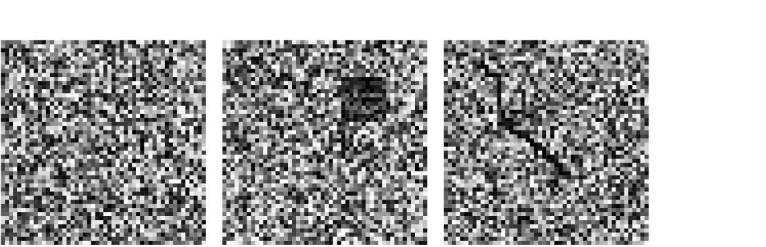
We are interested in the situation where the anomalous cluster $K$ is unknown, namely in testing $\mathbb{H}^{m}_{0}$ against $\mathbb{H}^{m}_{1}:=\bigcup_{K\in\mathcal{K}_{m}}\mathbb{H}^{m}_{1,K}$ . We illustrate the setting in Figure 1 in the context of the two-dimensional square grid.

Refer to caption — Figure 1: This figure illustrates the setting in dimension $d=2$ for a beta model where $F_{0}=\operatorname{Unif}(0,1)$ and $F_{\theta}=\operatorname{Beta}(\theta+1,1),\theta\geq 0$ . (Left) An instance of the null hypothesis. (Middle) An instance of an alternative with a square cluster. (Right) An instance of an alternative with a path.

Let $\mathcal{K}_{m}$ denote a cluster class for $\mathbb{V}_{m}$ . As usual, a test $T$ is a function of the data, $T=T(X_{v}\colon\ v\in\mathbb{V}_{m})$ , that takes values in $\{0,1\}$ , with $T=1$ corresponding to a rejection, meaning a decision in favor of $\mathbb{H}^{m}_{1}$ . For a test $T$ , we define its worst-case risk as the sum of its probability of type I error and its probability of type II maximized over the anomalous clusters in the class

\gamma_{m}(T)=\mathbb{P}(T=1|\mathbb{H}^{m}_{0})+\max_{K\in\mathcal{K}_{m}}\mathbb{P}(T=0|\mathbb{H}^{m}_{1,K}).

A method is formally defined as a sequence of tests $(T_{m})$ for testing $\mathbb{H}^{m}_{0}$ versus $\mathbb{H}^{m}_{1}$ . We say that a method $(T_{m})$ is asymptotically powerless if

\liminf_{m\to\infty}\gamma_{m}(T_{m})\geq 1.

This amounts to saying that as the size of the network increases, the method $(T_{m})$ is not substantially better than random guessing. Conversely, a method $(T_{m})$ is asymptotically powerful if

\lim_{m\to\infty}\gamma_{m}(T_{m})=0.

The minimax risk is defined as $\gamma_{m}^{*}:=\inf_{T}\gamma_{m}(T)$ , and we say that a method is $(T_{m})$ (asymptotically) optimal if $\gamma_{m}(T_{m})\to 0$ whenever $\gamma_{m}^{*}\to 0$ . Everything else fixed, the latter depends on the behavior of $\theta_{m}$ when $m$ becomes large. We say that $(T_{m})$ is optimal up to a multiplicative constant $C\geq 1$ if $\gamma_{m}(T_{m})\to 0$ under $C\theta_{m}$ whenever $\gamma_{m}^{*}\to 0$ under $\theta_{m}$ . We say that $(T_{m})$ is near-optimal if the same is true with $C$ replaced by $C_{m}\to\infty$ with $\log C_{m}=\mathrm{o}(\log\theta_{m})$ . (This occurs here only when $\theta_{m}\to 0$ polynomially fast and $C_{m}\to\infty$ poly-logarithmically fast.)

We focus on situations where the clusters in the class $\mathcal{K}_{m}$ are of same size, increasing with $m$ but negligible compared with the size of the entire network. We do so for the sake of simplicity; more general results could be obtained as in Arias-Castro, Candès and Durand [1], Arias-Castro, Donoho and Huo [3], Perone Pacifico et al. [45], Walther [54] without additional difficulty. Assuming a large anomalous cluster allows us to state general results applying to a wide range of one-parameter exponential families (via the central limit theorem). In addition, note that on the one hand, reliably detecting a cluster of bounded size is impossible in the Bernoulli model or any other model where $F_{0}$ has finite support, whereas on the other hand, detecting a cluster of size comparable to that of the entire network is in some sense trivial, given that the simple test based on the total sum $\sum_{v\in\mathbb{V}_{m}}X_{v}$ is optimal up to a multiplicative constant.

We consider two emblematic classes of clusters, in some sense at the opposite extremes:

•

Hypercube detection. Let $\mathcal{K}_{m}$ denote the class of hypercubes within $\mathbb{V}_{m}$ of sidelength $[m^{\alpha}]$ with $0<\alpha<1$ . This class is parametric, with the location of the hypercube the only parameter.
•

Path detection. Let $\mathcal{K}_{m}$ denote the class of loopless paths within $\mathbb{V}_{m}$ of length $[m^{\alpha}]$ with $0<\alpha<1$ . This class is nonparametric, in the sense that its cardinality is exponential in the length of the paths.

See Figure 1 for an illustration. (Note that a hypercube of side length $k$ may be seen as a loopless path of length $k^{d}$ .) Although we obtain results for both, our main focus is in the setting of hypercube detection, which is relevant to a wider range of applications, in fact any situation where the task is to detect a shape that is not filamentary. The situation exemplified in the setting of path detection may be relevant in target tracking from video, or the detection of cracks in materials in non-destructive testing. Note that the two settings coincide in dimension one.

We state fundamental detection bounds for each setting. The following result is standard (see, e.g., Arias-Castro, Candès and Durand [1]; Arias-Castro, Donoho and Huo [3]). Remember that $\sigma_{0}^{2}$ denotes the variance of $F_{0}$ .

Lemma 0

In hypercube detection, all methods are asymptotically powerless if

\limsup_{m\to\infty}(\log m)^{-1/2}m^{d\alpha/2}\theta_{m}<\sigma_{0}\sqrt{2d(1-\alpha)}.

In fact, the conclusions of Lemma 1 apply for a wide variety of parametric classes, such as discs, a popular model in disease outbreak detection (Kulldorff and Nagarwalla [33]), as well as to nonparametric classes of blob-like clusters (see Arias-Castro, Candès and Durand [1]; Arias-Castro, Donoho and Huo [3]).

The following result is taken from Arias-Castro et al. [2].

Lemma 0

In path detection, all methods are asymptotically powerless if $\lim_{m\to\infty}\theta_{m}\*(\log m)(\log\log m)^{1/2}=0$ , in dimension $d=2$ , and the same is true in dimension $d\geq 3$ if $\limsup_{m\to\infty}\theta_{m}<\theta_{*}$ , where $\theta_{*}>0$ depends only on $d$ .

In dimension $d\geq 4$ , $\theta_{*}$ may be taken to be the unique solution to

\rho\varphi(2\theta)-\varphi(\theta)^{2}=0,

where $\rho$ is the return probability of a symmetric random walk in dimension $d$ .

3 The scan statistic

For a subset of nodes $K\subset\mathbb{V}$ , let $|K|$ denote its size and define

\bar{X}_{K}=\frac{1}{|K|}\sum_{v\in K}X_{v}.

Given a cluster class $\mathcal{K}$ , we define the (simple) scan statistic as

\max_{K\in\mathcal{K}}\sqrt{|K|}(\bar{X}_{K}-\mu_{0}),

(1)

where $\mu_{0}$ is the mean of $F_{0}$ . If $\mu_{0}$ is not available, we may use the grand mean $\bar{X}_{\mathbb{V}_{m}}$ instead. In Appendix B, we derive this form of the scan statistic as an approximation to the scan statistic of Kulldorff [29], which is, strictly speaking, the GLR and arguably the most popular version, particularly in spatial statistics. We use this simpler form to streamline our theoretical analysis.

The test that rejects for large values of the scan statistic (1), which we call the scan test, is near-optimal in a wide range of settings (Arias-Castro, Candès and Durand [1]; Arias-Castro, Donoho and Huo [3]; Walther [54]). In particular, in the context of a class of hypercubes, and in fact many other parametric classes, this test is asymptotically optimal to the exact multiplicative constant.

Lemma 0

In hypercube detection, the scan test is asymptotically powerful if

\liminf_{m\to\infty}(\log m)^{-1/2}m^{d\alpha/2}\theta_{m}>\sigma_{0}\sqrt{2d(1-\alpha)}.

In the context of a class of paths, the following result states that the scan test detects if $\theta_{m}$ is bounded away from 0 and sufficiently large. Note that this does not match the order of magnitude of the lower bound given in dimension $d=2$ . Let $\Lambda(\theta)=\log\varphi(\theta)$ and $\Lambda^{*}(x)=\sup_{\theta\geq 0}[\theta x-\Lambda(\theta)].$ ( $\Lambda^{*}$ is the rate function of $F_{0}$ when $x\geq\mu_{0}$ .) The following result is established in Arias-Castro et al. [2].

Lemma 0

In path detection, the scan test is asymptotically powerful if

\liminf_{m\to\infty}\theta_{m}>\theta_{*}:=(\Lambda^{*}\circ\Lambda^{\prime})^{-1}(\log(2d)).

4 Size of the largest open cluster

We study the test based on the size of the largest connected component after thresholding the values at the nodes. This test was independently considered in a series of papers (Davies, Langovoy and Wittich [14]; Langovoy and Wittich [34]). Our results are seen to sharpen and elaborate on these results. In particular, we study this test under all three regimes (subcritical, supercritical, and critical).

Adapting terminology from percolation theory (Grimmett [21]), for a threshold $t\in\mathbb{R}$ , we say that a subset $K\subset\mathbb{V}$ is open (at threshold $t$ ) if $X_{v}>t$ for all $v\in K$ . Let $S_{m}(t)$ (resp., $S_{K}(t)$ ) denote the size of the largest open cluster within $\mathbb{V}_{m}$ (resp., within $K$ ). The analysis of the test based on $S_{m}(t)$ , which we call the largest open cluster (LOC) test, boils down to bounding the size of $S_{m}(t)$ from above, under $\mathbb{H}^{m}_{0}$ , and, because $S_{m}(t)\geq S_{K}(t)$ , bounding the size of $S_{K}(t)$ from below, under $\mathbb{H}^{m}_{1,K}$ . Define $\xi_{v}(t)=\mathbf{I}\{X_{v}>t\}$ , which is Bernoulli with parameter $p_{\theta}(t):=\mathbb{P}_{\theta}(X_{v}>t)$ . The process $(\xi_{v}(t)\colon\ v\in\mathbb{V}_{m})$ is a site percolation model (Grimmett [21]). In general, consider a process $(\xi_{v}\colon\ v\in\mathbb{V}_{m})$ i.i.d. Bernoulli with parameter $p$ , and let $S_{m}$ denote the size of the largest open cluster within $\mathbb{V}_{m}$ . In dimension $d=1$ , this process may be seen as a sequence of coin tosses, and $S_{m}$ viewed as the longest heads run in that sequence. In this context, the Erdős–Rényi Law (Erdős and Rényi [17]) says that

\frac{S_{m}}{\log m}\to\frac{1}{\log(1/p)},\qquad\mbox{almost surely}.

(2)

In higher dimensions $d\geq 2$ , the situation is much more involved. Let $p_{c}$ denote the critical probability for site percolation in $\mathbb{Z}^{d}$ , defined as the supremum over all $p\in(0,1)$ such that the size of the open cluster at the origin, denoted by $S$ , is finite with probability 1. (The dependency in $d$ is left implicit.) We consider the subcritical ( $p_{0}(t)<p_{c}$ ), supercritical ( $p_{0}(t)>p_{c}$ ), and near-critical ( $p_{0}(t)\approx p_{c}$ ) cases separately.

4.1 Subcritical percolation

In the subcritical case, where $t$ is such that $p_{0}(t)<p_{c}$ , we are able to obtain precise, rigorous results on the performance of the test based on $S_{m}(t)$ in terms of the function $\zeta_{p}$ , implicitly defined as

\zeta_{p}:=-\lim_{k\to\infty}\frac{1}{k}\log\mathbb{P}(S\geq k)=-\lim_{k\to\infty}\frac{1}{k}\log\mathbb{P}(S=k)

(3)

(see Grimmett [21], Section 6.3). Again, the dependency in $d$ is left implicit. As a function of $p\in(0,p_{c})$ , $\zeta_{p}$ is continuous and strictly decreasing, with limits $\infty$ at $p=0$ and 0 at $p=p_{c}$ (see Lemma 8), whereas $\zeta_{p}=0$ for $p\geq p_{c}$ . In the Appendix, we include a proof that

\frac{S_{m}}{\log m}\to\frac{d}{\zeta_{p}},\qquad\mbox{in probability}

(4)

for a subcritical threshold $p<p_{c}$ .

The convergence result in (4) may be used to bound $S_{m}(t)$ under the null by taking $p=p_{0}(t)$ . Under the alternative, if we consider a class of hypercubes, then (4) also may be used to bound $S_{K}(t)$ , because $K$ is a scaled version of $\mathbb{V}_{m}$ .

Theorem 1

In hypercube detection, the test based on $S_{m}(t)$ , with $t$ fixed such that $0<p_{0}(t)<p_{c}$ , is asymptotically powerful if $\liminf_{m\to\infty}\theta_{m}>\theta_{*}(t)$ , and asymptotically powerless if $\limsup_{m\to\infty}\theta_{m}<\theta_{*}(t)$ , where $\theta_{*}(t)$ is the unique solution to $\zeta_{p_{\theta}(t)}=\alpha\zeta_{p_{0}(t)}$ .

Note that when $t$ is fixed, $\zeta_{p_{\theta}(t)}$ as a function of $\theta$ is continuous and strictly strictly decreasing, by the fact that $p_{\theta}(t)$ is continuous and strictly increasing in $\theta$ (Brown [7], Cor. 2.6, 2.22) and $\zeta_{p}$ is continuous and strictly decreasing in $p$ (Lemma 8). Therefore, $\theta_{*}(t)$ in the theorem is well defined.

If instead, we consider a class of paths, then (2) may be used to bound $S_{K}(t)$ , because $K$ is a scaled version of the lattice in dimension 1. In congruence with (2), we define $\zeta^{1}_{p}=\log(1/p)$ .

Theorem 2

In path detection, the test based on $S_{m}(t)$ , with $t$ fixed such that $0<p_{0}(t)<p_{c}$ , is asymptotically powerful if $\liminf_{m\to\infty}\theta_{m}>\theta_{*}^{+}(t)$ , and asymptotically powerless if $\limsup_{m\to\infty}\theta_{m}<\theta_{*}^{-}(t)$ , where $\theta_{*}^{+}(t)$ (resp., $\theta_{*}^{-}(t)$ ) is the unique solution to $d\zeta^{1}_{p_{\theta}(t)}=\alpha\zeta_{p_{0}(t)}$ (resp., $d\zeta^{1}_{p_{\theta}(t)}=\alpha\zeta_{p_{0}(t)}$ ).

Note that in dimension $d\geq 2$ , the result is not sharp, because we always have $\theta_{*}^{+}(t)>\theta_{*}^{-}(t)$ . We believe that sharper forms of this result may be substantially more involved, and for this reason we have not pursued this.

Qualitatively, the message is that for both hypercube detection and path detection, the subcritical LOC test requires that $\theta_{m}$ be larger than a constant to be effective. Compared with the scan statistic, this makes it grossly suboptimal when detecting hypercubes and comparable (up to a multiplicative constant in $\theta_{m}$ ) when detecting self-avoiding paths.

What if we let $t=t_{m}\to\infty$ , so that $p_{0}(t_{m})\to 0$ ? Then the test based on $S_{m}(t_{m})$ is powerless under some additional conditions on $F_{0}$ . For $b,C\geq 0$ , consider the following class of approximately exponential power ( $\operatorname{AEP}$ ) distributions, sometimes called Subbotin distributions:

\operatorname{AEP}(b,C)=\{F\colon\ x^{-b}\log\bar{F}(x)\to-C,x\to\infty\}.

( $\bar{F}(x):=1-F(x)$ is the survival distribution function of $X\sim F$ .) For example, $\operatorname{Exp}(\lambda)\in\operatorname{AEP}(1,\lambda)$ and $\mathcal{N}(\mu,\sigma^{2})\in\operatorname{AEP}(2,1/(2\sigma^{2}))$ , whereas $\operatorname{Poi}(\lambda)$ behaves roughly as a distribution in $\operatorname{AEP}(1,C)$ .

Proposition 1

Assume that $F_{0}\in\operatorname{AEP}(b,C)$ for some $b>1$ and $C>0$ . In hypercube detection, the test based on $S_{m}(t)$ is asymptotically powerless when $t=t_{m}\to\infty$ , unless $\theta_{m}\to\infty$ .

4.2 Supercritical percolation

Here we consider the supercritical regime, where $p_{0}(t)>p_{c}$ . (Note that necessarily $d\geq 2$ for $p_{c}=1$ in dimension 1.) In this setting, too, the size of the largest cluster is well understood. Let $\Theta_{p}$ be the probability that the open cluster at the origin is infinite, and note that $\Theta_{p}>0$ for $p>p_{c}$ , by the definition of $p_{c}$ . We have with probability 1 that

\frac{S_{m}}{|\mathbb{V}_{m}|}\to\Theta_{p}

(see Falconer and Grimmett [18], Lemma 2 and proof, Penrose and Pisztora [44], Theorem 4, Pisztora [46]). In fact (with probability $1-\mathrm{o}(1)$ ), the largest open cluster within $\mathbb{V}_{m}$ is unique, and the foregoing statement says that it occupies a non-negligible fraction of $\mathbb{V}_{m}$ . With a supercritical choice of threshold, the LOC test is powerless for any $\theta$ if the anomalous cluster is too small, specifically if $\alpha<1/2$ in the setting of hypercube detection. Indeed, we have the following result.

Theorem 3

In hypercube detection, the test based on $S_{m}(t)$ , with $t$ fixed such that $p_{c}<p_{0}(t)<1$ , is asymptotically powerful if $\alpha\geq 1/2$ and $\lim_{m\to\infty}\theta_{m}m^{(\alpha-1/2)d}=\infty$ , and asymptotically powerless if $\alpha<1/2$ or if $\lim_{m\to\infty}\theta_{m}m^{(\alpha-1/2)d}=0$ .

Thus, for the detection of small clusters, a supercritical LOC test is potentially worthless, whereas for larger clusters it improves substantially on the performance of a subcritical LOC test, although it is still suboptimal compared with the scan statistic. (Indeed, comparing the exponents when $\alpha\geq 1/2$ , we have $(\alpha-1/2)d<\alpha d/2$ , because $\alpha<1$ .) We mention that in the context of path detection, the same arguments show that the LOC test for any choice of supercritical threshold is asymptotically powerless.

4.3 Critical percolation

If our goal is to choose a threshold $t$ so as to maximize the difference in size for the largest open cluster under the null and under an alternative, then we are necessarily in the neighborhood of the percolation phase transition, which is to say that $|p-p_{c}|$ is small. (Again, here we assume $d\geq 2$ .) The percolation model is not fully understood in the critical regime, which poses a serious obstacle to a rigorous statistical analysis. (See Grimmett [21], Chapter 9, for a general discussion of this percolation regime.) We base our discussion on the work of Borgs et al. [6]. Let $\pi_{m}(p)$ denote the probability that the open cluster at the origin reaches outside the box $[-m,m]^{d}$ , and let $\xi(p)$ denote the correlation length, defined as

\frac{1}{\xi(p)}:=-\lim_{m\to\infty}\frac{1}{m}\log\pi_{m}(p).

Note that, with $\xi$ thus defined, $\xi(p)<\infty$ if and only if $p<p_{c}$ . The critical exponent for (subcritical) correlation length is postulated to be

\nu:=-\lim_{p\nearrow p_{c}}\frac{\log\xi(p)}{\log|p-p_{c}|}.

It is not known whether the limit exists for all dimensions, but it is known that $0<\nu<\infty$ whenever it exists. It is shown in Borgs et al. [6] that, subject to the existence of this limit together with other scaling assumptions, when $p=p_{m}$ varies with $m$ ,

S_{m}\asymp_{\mathrm{P}}\cases{\log m,&\quad$\mbox{if, for some }\nu^{\prime}>\nu,m^{1/\nu^{\prime}}(p_{m}-p_{c})\to-\infty$,\cr m^{d},&\quad$\mbox{if, for some }\nu^{\prime}>\nu,m^{1/\nu^{\prime}}(p_{m}-p_{c})\to\infty$,}

(5)

where $X_{m}\asymp_{\mathrm{P}}Y_{m}$ means that there exists a constant $C\in(0,\infty)$ such that $C^{-1}\leq X_{m}/Y_{m}\leq C$ in probability. The scaling assumptions of Borgs et al. [6] are believed to hold if and only if the number $d$ of dimensions satisfies $2\leq d\leq 6$ , and they are proved for $d=2$ . The work of Borgs et al. [6] was directed at bond percolation only, but similar results are expected for site percolation.

It is known that $\nu=4/3$ for site percolation on the triangular lattice (see Smirnov and Werner [50]), and it is believed that this holds for percolation on any two-dimensional lattice. As described in Grimmett [21], Section 10.4, it is believed that $\nu=1/2$ for $d\geq 6$ , and this has been proved for $d\geq 19$ and for the so-called “spread-out model” in $7$ and more dimensions (Hara, van der Hofstad and Slade [23]).

Subject to the assumption that (5) holds, we establish the power of the test based on $S_{m}(t)$ when choosing $t=t_{m}$ near criticality. We assume that there exists $t_{c}$ such that $p_{0}(t_{c})=p_{c}$ , and that $p_{0}(t)$ is a continuous function of $t$ in a neighborhood of $t_{c}$ .

Theorem 4

Let $t_{m}\geq t_{c}$ be such that $p_{c}-p_{0}(t_{m})\asymp m^{-1/\nu^{\prime}}$ for some $\nu^{\prime}>\nu$ . In hypercube detection, assuming that (5) holds, the test based on $S_{m}(t_{m})$ is asymptotically powerful if $\liminf_{m\to\infty}\theta_{m}m^{\alpha/\nu^{\prime}}$ is sufficiently large.

Compared with a subcritical choice of threshold, which requires that $\theta_{m}$ be bounded away from 0 for the test to have any power, as seen in Theorem 1, with a near-critical choice of threshold, the test is able to detect at polynomially small $\theta_{m}$ . In particular, with a proper choice of threshold, the test is powerful for $\theta_{m}$ of order $m^{-\alpha/\nu^{\prime}}$ with $\nu^{\prime}>\nu$ . Note that, by Lemma 1, all methods are asymptotically powerless if $\theta_{m}$ is of order $m^{-d\alpha/2}$ , implying that $\alpha/\nu\leq d\alpha/2$ . We thus obtain the inequality $\nu\geq 2/d$ . This may be compared with the scaling relation (Grimmett [21], Equation (9.23)) stating that $d\nu=2-a$ , where $a$ ( $<0$ ) is the percolation critical exponent for the number of clusters per vertex. It is believed that $a=-\frac{2}{3}$ when $d=2$ and $a=-1$ when $d\geq 6$ . Compared with the performance at supercriticality, the test at near-criticality (with a proper choice of threshold) is superior if $(\alpha-\frac{1}{2})d<\alpha/\nu$ , which is equivalent to $\alpha<(1-a/2)/(1-a)$ . For example, with $a=-\frac{2}{3}$ , the near-critical LOC test is superior when $\alpha<\frac{3}{4}$ .

5 The upper level set scan statistic

For a threshold $t$ , let $\mathcal{Q}_{m}^{(t)}$ denote the (random) class of clusters within $\mathbb{V}_{m}$ open at $t$ , and let $\mathcal{Q}_{m}^{*}=\bigcup_{t}\mathcal{Q}_{m}^{(t)}$ , which is also random. Patil and Taillie [41] suggested scanning the clusters in $\mathcal{Q}_{m}^{*}$ . To facilitate a rigorous mathematical analysis of its performance, we consider the upper level set ( $\operatorname{ULS}$ ) scan at a given threshold $t$ , and use the simple scan described in Section 3. Specifically, in correspondence with (1), we define the (simple) $\operatorname{ULS}$ scan statistic at threshold $t$ as

U_{m}(t,k_{m})=\max\bigl{\{}\sqrt{|K|}(\bar{X}_{K}-\mu_{0|t})\colon\ K\in\mathcal{Q}_{m}^{(t)},|K|\geq k_{m}\bigr{\}},

(6)

where $\mu_{0|t}$ (resp., $\sigma^{2}_{0|t}$ ) is the the mean (resp., variance) of $X_{v}|X_{v}>t$ when $X_{v}\sim F_{0}$ , and $(k_{m})$ is a non-decreasing sequence of positive integers. The $\operatorname{ULS}$ scan statistic of Patil and Taillie [41] corresponds (in its simple form) to

\operatorname{ULS}_{m}=\max_{t\in\mathbb{R}}\frac{U_{m}(t,1)}{\sigma_{0|t}}.

(7)

If $\mu_{0|t}$ and/or $\sigma_{0|t}^{2}$ are not available, we may use their empirical versions based on the $X_{v}$ that survive the threshold $t$ . We restrict the scan to clusters of size at least $k_{m}$ to increase power, because the behavior of $U_{m}(t)$ is, as we show later, completely driven by the smallest open clusters that are scanned, at least when $t$ is subcritical. We present the rest of our discussion in terms of subcritical, supercritical, and near-critical choices of threshold. We then conclude with a result on the performance of the $\operatorname{ULS}$ scan test across all thresholds.

5.1 Subcritical threshold

We start by describing the behavior of $U_{m}(t,k_{m})$ under the null. Let $F_{\theta|t}$ denote the distribution of $X_{v}|X_{v}>t$ under $F_{\theta}$ , and let $\mu_{\theta|t}$ and $\Lambda^{*}_{\theta|t}$ denote its mean and rate function, respectively. Also, when $0<\beta<1/\zeta_{p_{\theta}(t)}$ , or $\beta=0$ and $F_{0}\in\operatorname{AEP}(b,C)$ for some $b\geq 2$ and $C>0$ , let $\gamma_{\theta|t}(\beta):=\gamma(F_{\theta|t},\mu_{0|t},\zeta_{p_{\theta}(t)},\beta)$ , where $\gamma$ is the function defined in Lemma 16. Note that $\gamma_{\theta|t}(\beta)$ can be computed explicitly in some cases, like the normal location model, and $\gamma_{\theta|t}(\beta)\sim(\mu_{\theta|t}-\mu_{0|t})^{2}/\zeta_{p_{\theta}(t)}$ when $\theta\nearrow\theta_{c}(t)$ , defined (when it exists) as the solution to $p_{\theta}(t)=p_{c}$ .

Lemma 0

Assume that $\theta\geq 0$ and $t$ is fixed such that $0<p_{\theta}(t)<p_{c}$ and that $k_{m}/\log m\to d\beta$ for some $\beta\geq 0$ . Then, under $F_{\theta}$ on $\mathbb{V}_{m}$ , the following holds in probability:

1.

If $\beta>1/\zeta_{p_{\theta}(t)}$ , then $U_{m}(t,k_{m})=0$ for $m$ large enough.
2.

If $0<\beta<1/\zeta_{p_{\theta}(t)}$ , then

$(\log m)^{-1/2}U_{m}(t,k_{m})\to(d\gamma_{\theta|t}(\beta))^{1/2}.$
3.
If $\beta=0$ and $F_{0}\in\operatorname{AEP}(b,C)$ for some $b\geq 1$ and $C>0$ , then
1. [(b)]
2. (a)
  
  If $b\geq 2$ , the convergence in Part 2 applies;
3. (b)
  
  If $b<2$ ,
  
  $k_{m}^{1/b-1/2}(\log m)^{-1/b}U_{m}(t,k_{m})\to(d/C)^{1/b}.$

In the last case, where $\beta=0$ , the behavior of $U_{m}(t)$ is influenced by the very large deviations of $F_{\theta|t}^{*k}$ for $k\geq k_{m}$ . (The symbol $*$ denotes convolution.) We choose to state a result for $\operatorname{AEP}$ distributions, for which the very large deviations resemble the large deviations.

Based on Lemma 5, we establish the performance of the $\operatorname{ULS}$ scan statistic. We start by arguing that choosing $k_{m}$ such that $k_{m}/\log m\to 0$ leads to a test that may potentially have less power than the test based on the largest cluster after thresholding. Indeed, the behavior of the $\operatorname{ULS}$ scan statistic does not depend on $\theta$ as long as $\theta<\theta_{c}(t)$ .

Proposition 2

Assume that $F_{0}\in\operatorname{AEP}(b,C)$ for some $b\in(1,2)$ and $C>0$ . In hypercube detection, the test based on $U_{m}(t,k_{m})$ , with $t$ fixed such that $0<p_{0}(t)<p_{c}$ and $k_{m}/\log m\to 0$ , is asymptotically powerless if $\limsup_{m\to\infty}\theta_{m}<\theta_{c}(t)$ .

For example, in the setting just described with $d=1$ , the $\operatorname{ULS}$ scan test has (asymptotically) no power unless $\theta_{m}\to\infty$ , whereas the test based on the size of the largest cluster after thresholding is, by Theorem 1, asymptotically powerful if $\liminf_{m\to\infty}\theta_{m}$ is large enough. We therefore choose a sequence $k_{m}$ comparable in magnitude to $\log m$ and state the performance of the $\operatorname{ULS}$ scan test in this case.

Theorem 5

In hypercube detection, the test based on $U_{m}(t,k_{m})$ , with $t$ fixed such that $0<p_{0}(t)<p_{c}$ and $k_{m}/\log m\to d\beta$ with $0<\beta<1/\zeta_{p_{0}(t)}$ , is asymptotically powerful if $\liminf_{m\to\infty}\theta_{m}>\theta_{*}(t)$ and asymptotically powerless if $\limsup_{m\to\infty}\theta_{m}<\theta_{*}(t)$ , where $\theta_{*}(t)$ is the unique solution to $\alpha\gamma_{\theta|t}(\beta)=\gamma_{0|t}(\beta)$ .

Note that $\theta_{*}(t)$ is well defined by Lemma 17 and that $\theta_{*}(t)<\theta_{c}$ as long as $\alpha>0$ . In any case, the test based on $U_{m}(t,k_{m})$ with a subcritical threshold $t$ is, in the setting of hypercube detection, asymptotically powerless when $\theta_{m}\to 0$ , just like the LOC test. In essence, the two tests are qualitatively comparable in this setting. This is also true in the context of path detection. Let $\gamma^{1}_{\theta|t}(\beta)$ denote $\gamma_{\theta|t}(\beta)$ in dimension 1.

Theorem 6

In path detection, the test based on $U_{m}(t,k_{m})$ , with $t$ fixed such that $0<p_{0}(t)<p_{c}$ and $k_{m}/\log m\to d\beta$ with $0<\beta<1/\zeta_{p_{0}(t)}$ , is asymptotically powerful if $\liminf_{m\to\infty}\theta_{m}>\theta_{*}^{+}(t)$ , and asymptotically powerless if $\limsup_{m\to\infty}\theta_{m}<\theta_{*}^{-}(t)$ , where $\theta_{*}^{+}(t)$ (resp., $\theta_{*}^{-}(t)$ ) is the unique solution to $\alpha\gamma^{1}_{\theta|t}(\beta)=\gamma_{0|t}(\beta)$ (resp., $\alpha\gamma_{\theta|t}(\beta)=\gamma_{0|t}(\beta)$ ).

As in Theorem 2, the result is not as sharp.

Qualitatively, we see that the performance of the subcritical $\operatorname{ULS}$ scan and LOC tests are comparable for both hypercube detection and path detection.

5.2 Supercritical threshold

Here we consider the choice of a supercritical threshold, where $t$ is fixed such that $p_{0}(t)>p_{c}$ . We already saw in Section 4.2 that the largest open cluster is unique and occupies a non-negligible fraction of the entire network. This is actually true both under the null and under an alternative. The $\operatorname{ULS}$ scan test based solely on the largest open cluster is comparable to the test based on the grand mean after thresholding. In turn, assuming $t$ is fixed, this test is asymptotically powerful when $m^{(\alpha-1/2)d}\theta_{m}\to\infty$ , and asymptotically powerless if $\alpha\leq 1/2$ and $\theta_{m}$ is bounded. (This is easily seen using Chebyshev’s inequality.) This is comparable to the LOC test at supercriticality.

In general, the $\operatorname{ULS}$ scan statistic includes other (smaller) open clusters. The story of the second-largest cluster of supercritical percolation in a box is not yet complete, and for this reason the behavior of the $\operatorname{ULS}$ scan statistic remains incompletely understood. The difficulty arises from the possibility that the second-largest cluster in $\mathbb{V}_{m}$ might lie at its boundary. Whether or not this occurs depends on the outcome of a calculation (yet to be done) of energy/entropy type involving so-called “droplets” near the boundary of $\mathbb{V}_{m}$ (see, e.g., Bodineau, Ioffe and Velenik [5]). To simplify the discussion, we finesse this problem by working where necessary on $\mathbb{V}_{m}$ with toroidal boundary conditions. That is, whenever we make statements concerning supercritical percolation on the graph $\mathbb{V}_{m}$ , we may add edges connecting sites on its boundary as follows: when $d=2$ , for $k=1,2,\ldots,m$ , an additional edge is placed between site $(1,k)$ and site $(m,k)$ , and similarly between $(k,1)$ and $(k,m)$ .

In proving exact asymptotics for test statistics under the null, we assume toroidal boundary conditions. Our results on asymptotic power do not require such exact results but require only orders of magnitude, which do not need the toroidal assumption. We emphasize that similar results are expected to hold with “free” (i.e., without the extra edges) rather than toroidal boundary conditions. Once the percolation picture is better understood, such results will follow in the same manner as those presented in this paper. Our results for the torus are also valid if instead we discount open clusters that touch the boundary of $\mathbb{V}_{m}$ . Details of this are omitted, and the proofs are essentially the same.

When working on the torus, the second-largest cluster is controlled through the following calculation. Cerf [8] proved that the limit

\delta_{p}:=-\lim_{k\to\infty}k^{-(d-1)/d}\log\mathbb{P}(\infty>S\geq k)=-\lim_{k\to\infty}k^{-(d-1)/d}\log\mathbb{P}(S=k),

(8)

exists, with $0<\delta_{p}<\infty$ for all fixed $p\in(p_{c},1)$ . The dependency on $d$ is left implicit.

A result similar to Lemma 5 holds with $\delta_{p}$ playing the role of $\zeta_{p}$ and the exponent of $\log m$ changed in places. It turns out that we need this result only when $\theta=0$ . For $\beta>0$ and a supercritical $t$ , let $\gamma_{0|t}(\beta):=\gamma(F_{0|t},\mu_{0|t},0,\beta)$ , defined in Lemma 16.

Lemma 0

Assume that $t$ is fixed such that $p_{c}<p_{0}(t)<1$ and that $k_{m}/\log m\to d\beta$ and $k_{m}^{(d-1)/d}/\log m\to d\beta^{\prime}$ for some $0\leq\beta,\beta^{\prime}\leq\infty$ . Then, under the null, the following holds in probability on the torus $\mathbb{V}_{m}$ :

1.

If $\beta^{\prime}>1/\delta_{p_{0}(t)}$ , then $U_{m}(t,k_{m})=\mathrm{O}(1)$ .

If $0\leq\beta^{\prime}<1/\delta_{p_{0}(t)}$ and $\beta=\infty$ , then

(\log m)^{-1/2}U_{m}(t,k_{m})\to\sigma_{0|t}\bigl{[}2d\bigl{(}1-\beta^{\prime}\delta_{p_{0}(t)}\bigr{)}\bigr{]}^{1/2},

where $\sigma_{0|t}^{2}:=\operatorname{Var}(F_{0|t})$ .

3.

If $\beta<\infty$ , then the conclusions of Lemma 5 apply. (Note that $\zeta_{p_{0}(t)}=0$ .)

Based on Lemma 6, we obtain the following result on the performance of the $\operatorname{ULS}$ scan test at supercriticality. As before, we restrict ourselves to the case where $U_{m}(t,k_{m})$ is of order $(\log m)^{1/2}$ . We also chose to state a simple result instead of a more precise result with multiple subcases. This result holds irrespective of the type of boundary condition assumed on $\mathbb{V}_{m}$ .

Theorem 7

In hypercube detection, the test based on $U_{m}(t,k_{m})$ , with $t$ fixed such that $p_{c}<p_{0}(t)<1$ and $\liminf k_{m}/\log m>0$ and $\limsup k_{m}^{(d-1)/d}/\log m<\alpha d/\delta_{p_{0}(t)}$ , is asymptotically powerful (resp., powerless) if

\theta_{m}\bigl{[}m^{(\alpha-1/2)d}+(\log m)^{d/(2d-2)}\bigr{]}(\log m)^{-1/2}\to\infty\qquad\mbox{(resp., $\to 0$)}.

We also mention that the equivalent of Theorem 6 holds here as well.

The improvement of the supercritical $\operatorname{ULS}$ scan test compared with the supercritical LOC test is a weaker requirement on $\theta_{m}$ by a logarithmic factor. Thus, this test’s performance is still much worse than that of the scan statistic when detecting hypercubes.

5.3 Critical threshold

If we choose a threshold as described in Section 4.3, and if (5) is true, then the power of the $\operatorname{ULS}$ scan statistic is greatly improved, as in the case of the LOC test. In fact, it can be proven that Theorem 4 remains valid with $S(t_{m})$ replaced with $U_{m}(t_{m},k_{m})$ , as long as $k_{m}=\mathrm{o}(m)^{\alpha d}$ so that the largest open cluster under the alternative is scanned. This boils down to showing that under the null, the $\operatorname{ULS}$ scan statistic is at most a power of $\log m$ , which we do in Lemma 7 below. However, the $\operatorname{ULS}$ scan test does not seem to offer any substantial gain in power over the LOC test, given that $\theta_{m}$ is still required to be large enough to change the regime of the percolation process within an alternative $K$ from subcritical to supercritical. That said, actually proving this would require information on the smaller open clusters near criticality, which is scarce and very difficult to obtain (see Borgs et al. [6] for some partial results and postulates).

5.4 Across all thresholds

Finally, we discuss the (simple) $\operatorname{ULS}$ scan test across all thresholds, as suggested in Patil and Taillie [41]. To take advantage of a phase transition near criticality, we assume, as in Section 4.3, that there exists $t_{c}$ such that $p_{0}(t_{c})=p_{c}$ and that $p_{0}(t)$ is a continuous function of $t$ in a neighborhood of $t_{c}$ . We also assume that (5) holds. In Proposition 2, we showed that scanning small clusters may lead to a decrease in power. For this reason, and also to facilitate the analysis, we limit ourselves to clusters of size at least $k_{m}$ ; that is, we consider the test based on

\operatorname{ULS}_{m}(k_{m})=\max_{t\in\mathbb{R}}\frac{U_{m}(t,k_{m})}{\sigma_{0|t}},

(9)

where, for definiteness, $U_{m}(t,k_{m})$ is calculated on the torus $\mathbb{V}_{m}$ when $t<t_{c}$ .

Let $\Gamma_{\theta}(\beta)=\inf_{t}\gamma_{\theta|t}(\beta)/\sigma_{0|t}^{2}$ , where, in congruence with Sections 5.1 and 5.2,

\gamma_{\theta|t}(\beta)=\cases{\gamma\bigl{(}F_{\theta|t},\mu_{0|t},\zeta_{p_{\theta}(t)},\beta\bigr{)},&\quad$t>t_{c}$,\cr\gamma(F_{\theta|t},\mu_{0|t},0,\beta),&\quad$t<t_{c}$,}

with $\gamma$ being the function defined in Lemma 16. We first establish the behavior of $\operatorname{ULS}_{m}(k_{m})$ under the null.

Lemma 0

Let $k_{m}=\beta\log m$ where $\beta>0$ , and let $t_{\beta}$ be such that $d/\beta\leq\zeta_{p_{0}(t_{\beta})}<\infty$ . Define $\eta(\beta):=\sup\{\sigma_{0|t}/\sigma_{0|s}\colon\ s\leq t\leq t_{\beta}\}$ . With probability tending to 1, under $F_{0}$ ,

\limsup_{m\to\infty}(\log m)^{-1/2}\operatorname{ULS}_{m}(k_{m})\leq\eta(\beta)(d\Gamma_{\theta}(\beta))^{1/2}.

If in addition, either $\sigma_{0|t}$ is non-decreasing in $t$ or $F_{0}$ has no atoms on $(-\infty,t_{\beta}]$ , then, in probability under $F_{0}$ ,

(\log m)^{-1/2}\operatorname{ULS}_{m}(k_{m})\to(d\Gamma_{\theta}(\beta))^{1/2}.

In fact, a result as precise as Lemma 7 is superfluous, given the behavior of the $\operatorname{ULS}$ scan statistic under the alternative at supercriticality and near-criticality, which is polynomial in $m$ . The next theorem does not require the use of toroidal boundary conditions.

Theorem 8

In hypercube detection and assuming that (5) holds, the test based on $\operatorname{ULS}_{m}(k_{m})$ , with $k_{m}=[\beta\log m]$ for some $\beta>0$ , is asymptotically powerful if $\theta_{m}m^{\lambda}\to\infty$ , for some $0<\lambda<\alpha/\nu$ satisfying $\lambda<(\alpha-1/2)d$ if $\alpha>1/2$ .

Thus, scanning all thresholds elicits the best performance of the LOC tests. Nevertheless, the overall test is still suboptimal when detecting hypercubes compared with the scan statistic. We mention in passing that the same result holds for the simpler test that scans only the largest open cluster at each threshold.

6 Implementation and numerical experiments

The scan test has been shown to be near-optimal in a wide variety of settings, differing in terms of both network structure and cluster class (Arias-Castro, Candès and Durand [1]; Arias-Castro, Donoho and Huo [3]). It is computationally demanding, however. For the simple situation of detecting a hypercube, the scan statistic can be computed in $\mathrm{O}(N\log N)$ flops, where $N:=m^{d}$ is the network size if the size of the hypercube is known. If one scans over all possible hypercubes, then computing the scan statistic requires $\mathrm{O}(N^{2}\log N)$ flops. For nonparametric shapes, the computational cost is even higher; in fact, for the problem of detecting a loopless path, computing the scan statistic corresponds to the reward-budget problem of DasGupta et al. [13], shown there to be NP-hard. Because the scan statistic is so computationally burdensome, the cluster class is most often taken to be parametric in practice, even though the underlying clusters may take a much wider range of shapes. For instance, discs are the prevalent shape used in disease outbreak detection (Kulldorff and Nagarwalla [33]), with variants such as ellipses (Hobolth, Pedersen and Jensen [26]; Kulldorff et al. [32]). For a wide range of parametric shapes, Arias-Castro, Donoho and Huo [3] recommended a multiscale approximation to the scan statistic. Efforts to move beyond parametric models include tree-based approaches (Kulldorff, Fang and Walsh [31]), simulated annealing (Duczmal and Assunção [16]) and an exhaustive search among arbitrarily shaped clusters of small size (Tango and Takahashi [51]).

The LOC test does not assume any parametric form for the anomalous cluster, and in that sense is nonparametric. Its computational complexity at a given threshold is of order the number of nodes plus the number of edges in the network (Cormen et al. [10]), and so of order $\mathrm{O}(N)$ flops for the square lattice.

The $\operatorname{ULS}$ scan statistic is nonparametric as well. Computing $U_{m}(t,k_{m})$ requires determining $\mathcal{Q}_{m}^{(t)}$ , which takes $\mathrm{O}(N)$ flops, and then scanning over $\mathcal{Q}_{m}^{(t)}$ . Because the clusters in $\mathcal{Q}_{m}^{(t)}$ do not intersect, scanning over them takes order $\mathrm{O}(N)$ flops. Therefore, computing $\operatorname{ULS}_{m}$ can be done in $\mathrm{O}(M\cdot N)$ flops, where $M$ is the number of distinct values at the nodes. Patil and Taillie [42] argued that this can be done faster by using the tree structure of $\mathcal{Q}_{m}^{*}$ , where the root is the entire network $\mathbb{V}_{m}$ and a cluster $K\in\mathcal{K}_{m}(t_{j})$ is the parent of any cluster $L\in\mathcal{K}_{m}(t_{j+1})$ such that $L\subset K$ , where $t_{1}<\cdots<t_{M}$ denote the distinct values at the nodes.

We complement our theoretical analysis with some small-scale numerical experiments. Specifically, we explore the power properties of the LOC test of Section 4 and the $\operatorname{ULS}$ scan test of Section 5 in the context of detecting a hypercube in the two-dimensional square lattice. Patil, Modarres and Patankar [40] are developing sophisticated software implementing the $\operatorname{ULS}$ scan statistic for use in real-life situations, with more recent variations Patil, Joshi and Koli [38]. However, this software is not yet available, so we implemented our own (basic) routines.

We used the statistical software R (R Core Team [48]) with the package igraph (Csardi [11]). Our (basic) implementation of the $\operatorname{ULS}$ scan statistic for a given threshold is much slower than both the scan statistic with a given mask and the LOC statistic, especially when there is no constraint on the size of the open clusters to be scanned, that is, when $k_{m}=1$ . In all of our experiments, we chose the square lattice in dimension $d=2$ with side length $m=500$ for a total of 250,000 nodes, and we considered three alternatives: squares of side length $\ell\in\{10,50,100\}$ , corresponding roughly to $\alpha\in\{0.4,0.7,0.8\}$ . The squares were fixed away from the boundary of the lattice, given that the methods are essentially location-independent. (This is rigorously true of the scan statistic.) We assessed the performance of a method in a given situation by estimating its risk, which we define as the sum of the probabilities of type I and type II errors optimized over all rejection regions.

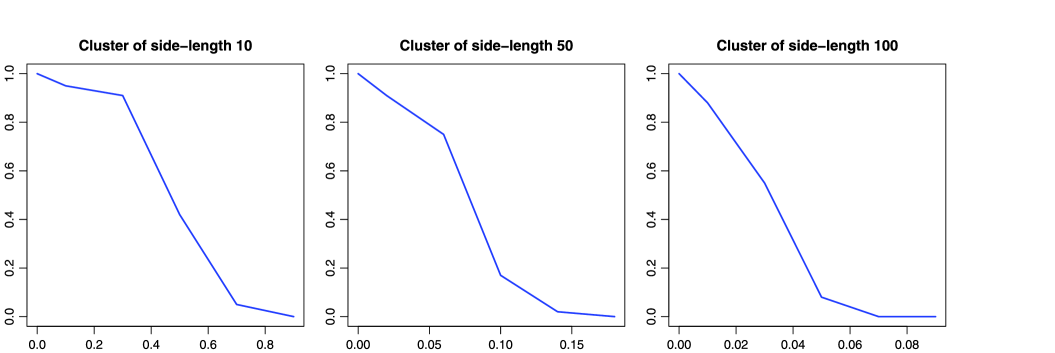
We first ran some experiments to quickly assess the power of the scan test. We found that the test agrees very well with the theory (i.e., Lemma 3), which we already knew from previous experience. Specifically, we assumed a normal location model and simulated 100 realizations of the null and each of the three alternatives with $\theta\in\{j/\ell\colon\ j=1,3,5,7,9\}$ (see Figure 2).

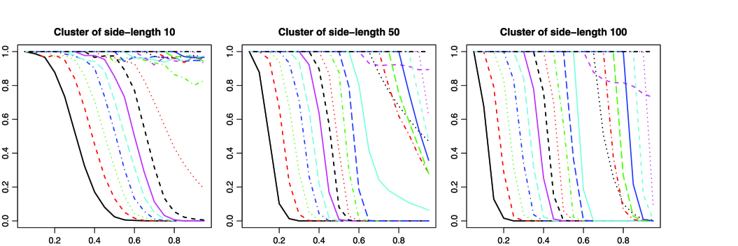
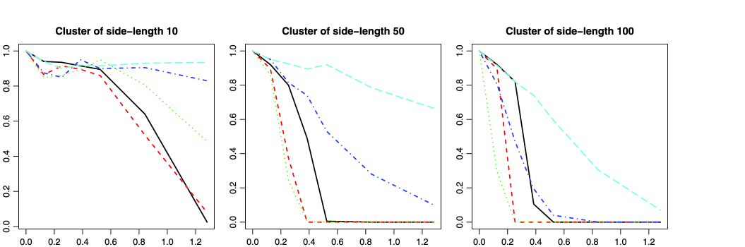
Next, we performed some larger experiments to assess the power of the LOC test. We simply assumed a site percolation model with probability $p\in\{0.05,0.10,\ldots,0.90,0.95\}$ . Note that $p_{c}$ is not known for site percolation in the square lattice, although $p_{c}\approx 0.593$ from extensive numerical experiments (Feng, Deng and Blöte [19]). We simulated the null and each of the three alternatives with $q\in\{0.05,0.10,\ldots,0.90,0.95\},q>p,$ within the anomalous cluster. We replicated each situation 1000 times. The risk curves are shown in Figure 3. The test seems to behave similarly above and below criticality. At near-criticality, the test is rather erratic. However, when the size of the anomalous cluster is large enough, $\ell=100$ , the risk curve is steepest just under $p_{c}$ , at $p=0.55$ in our experiments, with full power against $q\geq 0.65$ . Figure 4 shows boxplots of the test statistic for the case where $\ell=100$ and $p=0.40$ (subcritical), $p=0.55$ (near-critical), and $p=0.70$ (supercritical).

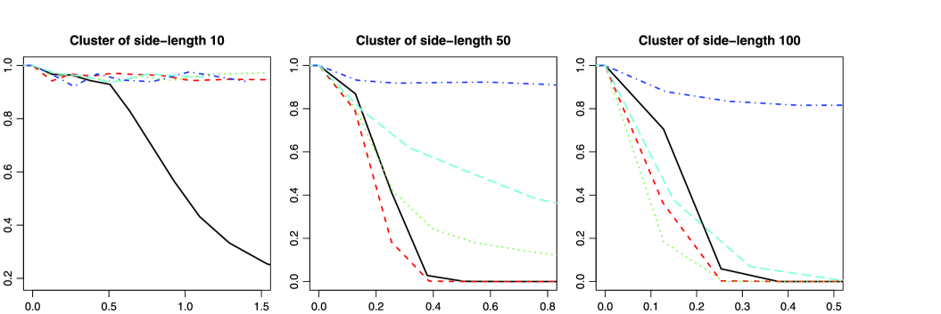
If we were to use this test in the context of a normal location model, then the correspondence would be $t=\bar{\Phi}^{-1}(p)$ (the threshold) and $\theta=t-\bar{\Phi}^{-1}(q)$ , where $\bar{\Phi}$ denotes the normal survival distribution function. Figure 5 plots the risk curves in this context for $p\in\{0.40,0.50,0.55,0.60,0.70\}$ . In particular, the test at near-criticality with $t=\bar{\Phi}^{-1}(0.55)=-0.126$ has full power against the alternative with $\ell=100$ and $\theta=0.26$ .

Finally, we experimented with the $\operatorname{ULS}$ scan test. To limit the size of our simulations, we considered alternatives with $\theta=\Phi^{-1}(q)$ with $q\in\{0.55,0.6,0.65,0.70,0.80,0.90\}$ and chose $t=\Phi^{-1}(p)$ with $p\in\{0.40,0.50,0.55,0.60,0.70\}$ as thresholds. We restricted scanning to open clusters of size not smaller than $1/10$ of the size of largest open cluster, essentially falling in the regime of Part 2 of Lemma 5, and also making the computation much faster. We used 200 replicates. We again see that the risk curve is sharpest near criticality when the size of the anomalous cluster is sufficiently large, here for $\ell\geq 50$ . Compared with the LOC test, the $\operatorname{ULS}$ scan test has more power at large $\theta$ when the cluster is small $\ell=10$ (as predicted) and, more interestingly, slightly more power when the cluster is larger. Compared with the scan statistic, which knows the size and shape of the anomalous cluster, the $\operatorname{ULS}$ scan test with the best choice of threshold (corresponding to $p=0.55$ ) requires approximately threefold greater signal amplitude.

7 Discussion

The contribution of this paper is a rigorous mathematical analysis of the performance of the LOC test independent of, and more extensively than Davies, Langovoy and Wittich [14] and Langovoy and Wittich [34], and of the $\operatorname{ULS}$ scan test, both nonparametric and computationally tractable methods. We made abundant use of percolation theory to establish these results. We compared the power of these tests with that of the scan statistic, which is known to be near-optimal in a wide array of settings. Although these tests are comparable in power with the scan statistic for the detection of a path, they may be substantially less powerful for the detection of a hypercube. Note, however, that the scan statistic is provided with knowledge about the shape and size of the anomalous cluster. In theory, we argued that this was the case based on some heuristics and conjectures from percolation theory. Numerically, this appears to be the case when the anomalous cluster is large enough. In our experiments, the $\operatorname{ULS}$ scan test was slightly more powerful than the LOC test, and required a $\theta$ three to four times larger than the scan statistic, which has the advantage of knowing the shape and size of the cluster. This result is promising, and further numerical experiments are needed to evaluate the power of these tests in truly nonparametric settings, because they do not require previous information about cluster shape, and are computationally more feasible in general.

Our theoretical results generalize to other networks that resemble the lattice, with a different critical percolation probability $p_{c}$ and different functions $\zeta_{p}$ and $\delta_{p}$ . In particular, we used the self-similarity property of the square lattice and the fact that it has polynomial growth. Our results also generalize to other cluster classes; in the setting of the square lattice, they extend immediately to any class of clusters that includes a hypercube of comparable size (e.g., the class $\mathcal{K}_{m}$ of clusters $K$ of size $|K|=[m^{\alpha}]^{d}$ ), such that there is a hypercube $K_{0}\subset K$ with $|K_{0}|/|K|\geq\omega_{m}$ , where $\omega_{m}\to 0$ more slowly than any negative power of $m$ . In addition, the class might contain clusters of different sizes, although in that case the worst-case risk would be driven by the smallest clusters. Implementation of the scan statistic may be much more demanding in this case. The main results of Section 4 require only that $F_{\theta}(t)$ be twice differentiable in $(t,\theta)$ , with $\partial_{\theta}F_{\theta}(t)<0$ for all $(t,\theta)$ , which is the case, for example, for location models and scale models if $F_{0}$ is twice differentiable with a strictly positive first derivate. With some additional work, we also can obtain results for classes of “thin” clusters as defined in Arias-Castro, Candès and Durand [1]. The key is to understand the percolation behavior within and near such clusters. Some results are available for slabs (Grimmett [21], Theorem 7.2) and more general subgraphs of lattices including “wedges,” and these appear to be transferable to other “curved” slabs.

Appendix A: Proofs

{nota*}

We write $f_{m}\sim g_{m}$ as $n\to\infty$ if $f_{m}/g_{m}\to 1$ . Similarly, we use $\mathrm{O}(\cdot)$ and $\mathrm{o}(\cdot)$ and write $f_{m}\asymp g_{m}$ as $n\to\infty$ if $f_{m}=\mathrm{O}(g_{m})$ and vice versa. We also use their random counterparts, $\sim_{\mathrm{P}}$ , $\asymp_{\mathrm{P}}$ , $\mathrm{O}_{\mathrm{P}}(\cdot)$ , and $\mathrm{o}_{\mathrm{P}}(\cdot)$ . For example, $Z_{m}=\mathrm{o}_{\mathrm{P}}(k_{m})$ means that $Z_{m}/k_{m}\to 0$ in probability, and $Z_{m}=\mathrm{O}_{\mathrm{P}}(k_{m})$ means that $Z_{m}/k_{m}$ is bounded in probability, which is to say that $\mathbb{P}(|Z_{m}|\geq k_{m}l_{m})\to 1$ as $m\to\infty$ for any $l_{m}$ satisfying $l_{m}\to\infty$ . We use $1\{A\}$ to denote the indicator function of the set $A$ . The maximum of $k$ and $\ell$ is denoted by $k\vee\ell$ .

.1 On the size of percolation clusters

Here we state and prove some results on the sizes of percolation clusters in $\mathbb{Z}^{d}$ . We start by proving some properties of $\zeta_{p}$ . Recall that $S$ denotes the size of the open cluster at the origin. Besides the limit in (3), the following bound holds for $p<p_{c}$ and all $k\geq 1$ :

\mathbb{P}_{p}(S\geq k)\leq(1-p)^{2}\frac{k\mathrm{e}^{-k\zeta_{p}}}{(1-\mathrm{e}^{-\zeta_{p}})^{2}},

(1)

by Grimmett [21], Equation (6.80), adapted to site percolation.

Lemma A.0

The function $\zeta_{p}$ defined in (3) is continuous and strictly decreasing over $(0,p_{c}]$ , and satisfies $\lim_{p\to 0}\zeta_{p}=\infty$ and $\lim_{p\to p_{c}}\zeta_{p}=0$ .

Proof.

Let $0\leq p<p^{\prime}\leq 1$ . By coupling $\mathbb{P}_{p}$ and $\mathbb{P}_{p^{\prime}}$ in the usual way,

\mathbb{P}_{p}(S=k)\geq(p/p^{\prime})^{k}\mathbb{P}_{p^{\prime}}(S=k),

so that $\zeta_{p}\leq\zeta_{p^{\prime}}+\log(p^{\prime}/p)$ . Applying Grimmett [21], Theorem 2.38, to the event $\{S\geq k\}$ , we find that, as in the proof of Grimmett [21], Equation (6.16), $\zeta_{p}/\log p\leq\zeta_{p^{\prime}}/\log p^{\prime}$ . In summary,

\zeta_{p}\biggl{(}1-\frac{\log(1/p^{\prime})}{\log(1/p)}\biggr{)}\leq\zeta_{p}-\zeta_{p^{\prime}}\leq\log(p^{\prime}/p).

(2)

Therefore, $\zeta_{p}$ is continuous and strictly decreasing on $(0,p_{c})$ . Moreover, by fixing $p^{\prime}\in(0,p_{c})$ and letting $p\to 0$ , we have

\zeta_{p}\geq\zeta_{p^{\prime}}\frac{\log(1/p)}{\log(1/p^{\prime})}\to\infty.

Finally, by Grimmett [21], Equations (6.83), (6.56), $\zeta_{p}\to 0=\zeta_{p_{c}}$ as $p\uparrow p_{c}$ . ∎

Next, we prove (4). We do this by standard means, and the claim may be strengthened (see also Grimmett [22]; Hofstad and Redig [52]).

Lemma A.0

Consider site percolation on $\mathbb{Z}^{d}$ with parameter $p<p_{c}$ , and let $S_{m}$ denote the size of the largest open cluster within $\mathbb{V}_{m}$ . Then (4) holds, namely

\frac{S_{m}}{\log m}\to\frac{d}{\zeta_{p}},\qquad\mbox{in probability}.

Proof.

Fix $0<\varepsilon<1/2$ . Let $S^{v}$ be the size of the open cluster at a node $v\in\mathbb{Z}^{d}$ , which has the same distribution as $S$ . We start with the upper bound. By the union bound,

\mathbb{P}(S_{m}\geq k)\leq\sum_{v\in\mathbb{V}_{m}}\mathbb{P}(S^{v}\geq k)=|\mathbb{V}_{m}|\cdot\mathbb{P}(S\geq k).

(3)

Thus, using (3), for $k_{m}(\varepsilon):=(1+\varepsilon)(d/\zeta_{p})\log m$ and $m$ large enough,

\mathbb{P}\bigl{(}S_{m}\geq k_{m}(\varepsilon)\bigr{)}\leq m^{d}\exp\bigl{(}-(1-\varepsilon/2)\zeta_{p}k_{m}(\varepsilon)\bigr{)}\leq m^{-\varepsilon d/4},

and the term on the right-hand side converges to $0$ .

For the lower bound, consider $N=\lceil m^{d}/(\log m)^{2d}\rceil$ nodes $v_{1},\ldots,v_{N}\in\mathbb{V}_{m}$ separated from each other and the boundary of $\mathbb{V}_{m}$ by at least $\frac{1}{2}(\log m)^{2}$ . Let $k_{m}(\varepsilon):=(1-\varepsilon)(d/\zeta_{p})\log m$ . For sufficiently large $m$ , the events $E_{i}:=\{|S^{v_{i}}|\leq k_{m}(\varepsilon)\}$ are independent. Therefore, using (3), for large $m$ ,

$\displaystyle\mathbb{P}\bigl{(}S_{m}\leq k_{m}(\varepsilon)\bigr{)}$	$\displaystyle\leq$	$\displaystyle\bigl{(}1-\mathbb{P}\bigl{(}S\geq k_{m}(\varepsilon)\bigr{)}\bigr{)}^{N}$
	$\displaystyle\leq$	$\displaystyle\bigl{(}1-\exp\bigl{(}-(1+\varepsilon/2)\zeta_{p}k_{m}(\varepsilon)\bigr{)}\bigr{)}^{N}$
	$\displaystyle\leq$	$\displaystyle\exp\bigl{(}-m^{\varepsilon d/2}/(\log m)^{2d}\bigr{)},$

and the last term on the right-hand side tends to 0 as $m\to\infty$ . ∎

The following result describes the behavior of size of the open cluster at the origin when $p$ is small. It may be made more precise, but we do not pursue this here.

Lemma A.0

There exists $c>0$ depending only on $d$ such that, for $p\in(0,(2c)^{-1})$ ,

p^{k}\leq\mathbb{P}_{p}(S\geq k)\leq{\textstyle\frac{1}{2}}(cp)^{k}\qquad\forall k\geq 1.

Proof.

An animal is a connected subgraph of $\mathbb{Z}^{d}$ containing the origin. The lower bound comes from considering the probability that any given animal of size $k$ is open. For the upper bound, by the union bound, we have $\mathbb{P}_{p}(S=k)\leq|\mathcal{A}_{k}|p^{k}$ , where $\mathcal{A}_{k}$ is the set of animals with $k$ vertices. There is a constant $c>0$ such that $|\mathcal{A}_{k}|\leq c^{k}$ , so that

\mathbb{P}_{p}(S\geq k)\leq\sum_{\ell\geq k}c^{\ell}p^{\ell}={\displaystyle\frac{(cp)^{k}}{1-cp}}\leq\frac{1}{2}(cp)^{k},

when $cp<\frac{1}{2}$ . ∎

We next present a result on the number of open clusters of a given size that is valid for all $p\in(0,1)$ .

Lemma A.0

Consider site percolation on $\mathbb{Z}^{d}$ with parameter $p$ , and let $N_{m}(k)$ denote the number of open clusters of size $k$ within $\mathbb{V}_{m}$ . Then, for $k\geq 1$ ,

\frac{(m-2k)^{d}}{k}\mathbb{P}(S=k)\leq\mathbb{E}(N_{m}(k))\leq\frac{m^{d}}{k}\mathbb{P}(\infty>S\geq k),

In addition, for $k,\ell\geq 1$ ,

\bigl{|}\operatorname{Cov}(N_{m}(k),N_{m}(\ell))\bigr{|}\leq 3^{d+1}(k+\ell)^{d}\mathbb{E}(N_{m}(k\vee\ell)).

Thus, for $k\geq 1$ ,

\operatorname{Var}(N_{m}(k))\leq 6^{d+1}k^{d}\mathbb{E}(N_{m}(k)).

Proof.

Let $S^{v}_{m}$ be the size of the open cluster at $v$ within the box $\mathbb{V}_{m}$ . Then

N_{m}(k)=\sum_{v\in\mathbb{V}_{m}}X^{v}(k),

(5)

where $X^{v}(k)=k^{-1}1\{S^{v}_{m}=k\}$ . We immediately have

\mathbb{E}(N_{m}(k))\leq\sum_{v\in\mathbb{V}_{m}}\frac{1}{k}\mathbb{P}(\infty>S^{v}\geq k)=\frac{|\mathbb{V}_{m}|}{k}\mathbb{P}(\infty>S\geq k).

For the lower bound, we count only nodes away from the boundary, obtaining

\mathbb{E}(N_{m}(k))\geq|\mathbb{V}_{m}(k)|\frac{1}{k}\mathbb{P}(S=k),

where $\mathbb{V}_{m}(k):=\{k,\ldots,m-k\}^{d}$ .

We turn now to the covariances. By (5),

	$\displaystyle\operatorname{Cov}(N_{m}(k),N_{m}(\ell))$	$\displaystyle=$	$\displaystyle\sum_{v,w\in\mathbb{V}_{m}}\operatorname{Cov}(X^{v}(k),X^{w}(l))$
		$\displaystyle=$	$\displaystyle\mathop{\mathop{\sum}_{v,w\in\mathbb{V}_{m}}}_{\\|v-w\\|\leq k+\ell}\operatorname{Cov}(X^{v}(k),X^{w}(l)),$

because $X^{v}(k)$ and $X^{w}(\ell)$ are independent if $\|v-w\|>k+\ell$ , where $\|\cdot\|$ denotes $\ell^{\infty}$ -norm. Now,

	$\displaystyle\bigl{\|}\operatorname{Cov}(X^{v}(k),X^{w}(\ell))\bigr{\|}$	$\displaystyle=$	$\displaystyle\bigl{\|}\mathbb{E}\bigl{(}X^{w}(\ell)\|X^{v}(k)=k^{-1}\bigr{)}-\mathbb{E}(X^{w}(\ell))\bigr{\|}\mathbb{E}(X^{v}(k))$
		$\displaystyle\leq$	$\displaystyle\frac{1}{\ell}\mathbb{E}(X^{v}(k)),$

so that

\bigl{|}\operatorname{Cov}(N_{m}(k),N_{m}(\ell))\bigr{|}\leq\frac{1}{\ell}(2k+2\ell+1)^{d}\mathbb{E}(N_{m}(k)),

and the second claim of the lemma follows. ∎

We now describe some properties of the open clusters within $\mathbb{V}_{m}$ in the supercritical regime. In this regime, it is known that, with probability 1, there is a unique infinite open cluster in $\mathbb{Z}^{d}$ , denoted by $Q_{\infty}$ (see, e.g., Grimmett [21], Section 8.2). With high probability, the largest open cluster within $\mathbb{V}_{m}$ is a subgraph of this infinite open cluster. Next, we present some additional information on its size, $S_{m}$ .

Lemma A.0

Suppose that $p>p_{c}$ . There is a constant $C>0$ such that, with probability at least $1-\exp(-Cm^{d-1})$ , there is a unique largest open cluster within $\mathbb{V}_{m}$ , and it is a subgraph of $Q_{\infty}$ . Moreover, as $m\to\infty$ , its size $S_{m}$ satisfies

\frac{S_{m}-\mathbb{E}(S_{m})}{\sqrt{\operatorname{Var}(S_{m})}}\to\mathcal{N}(0,1),\qquad\mbox{in distribution},

with $\mathbb{E}(S_{m})\sim\Theta_{p}|\mathbb{V}_{m}|$ and $\operatorname{Var}(S_{m})\sim\sigma^{2}|\mathbb{V}_{m}|$ for some $\sigma^{2}>0$ depending on $(d,p)$ .

Proof.

For the first part and the limiting behavior of $\mathbb{E}(S_{m})$ as $m\to\infty$ , see the discussion of Penrose and Pisztora [44], Theorems 4 and 6, and the beginning of this Appendix. For the weak limit and the limit size of the variance of $S_{m}$ , see, for example, Penrose [43], Theorem 3.2. ∎

We next describe some properties of the smaller open clusters. Let $S_{m}^{(2)}$ be the size of the largest open cluster of $\mathbb{Z}^{d}$ that is contained entirely within $\mathbb{V}_{m}$ .

Lemma A.0

Suppose that $p>p_{c}$ . There exists a positive constant $\delta_{p}$ such that

\frac{S_{m}^{(2)}}{(\log m)^{d/(d-1)}}\to\biggl{(}\frac{d}{\delta_{p}}\biggr{)}^{d/(d-1)},\qquad\mbox{in probability}.

For any $c>0$ , there exists $\sigma_{i}=\sigma_{i}(p,c)>0$ such that the following holds: With probability tending to 1, there exist at least $\sigma_{1}m^{d}\exp[-\sigma_{2}(\log m)^{(d-1)/d}]$ open clusters of size $[c\log m]$ of $\mathbb{Z}^{d}$ lying within $\mathbb{V}_{m}$ .

Our results on exact asymptotics in the supercritical phase concern $\mathbb{V}_{m}$ with toroidal boundary conditions. One effect of removing the boundary from $\mathbb{V}_{m}$ is that the asymptotics of the largest cluster coincide with those of $S_{m}$ , as well as for the second-largest cluster $S_{m}^{(2)}$ . In the proof of Theorem 7, we need an upper bound on the size of the second-largest cluster inside a box with “free” boundary conditions. We do not explore this in detail here, because it relies on extensions of arguments of Kesten and Zhang [28] (see also Grimmett [21], Proof of Theorem 8.65), which have not yet been not fully explored in the literature. Instead, we note that the the second-largest open cluster in a supercritical percolation model on $\mathbb{V}_{m}$ with free boundary conditions has size of order $\mathrm{O}_{\mathrm{P}}((\log m)^{d/(d-1)})$ . {pf*}Proof of Lemma 13 It was proven by Cerf [8] that the limit

\delta_{p}:=-\lim_{k\to\infty}k^{-(d-1)/d}\log\mathbb{P}(S=k)

(6)

exists and is strictly positive and finite when $p_{c}<p<1$ . It is elementary that $\delta_{p}$ thus defined is equal to that of (8) (see also Grimmett [21], Section 8.6). The first part of the lemma follows by the same proof as used in Lemma 9.

As in the proof of Lemma 11, the mean number $\mu_{m}$ of clusters of size $k:=[c\log m]$ satisfies

\frac{m^{d}}{c\log m}\exp\bigl{(}-\delta^{1}(c\log m)^{(d-1)/d}\bigr{)}\leq\mu_{m}\leq\frac{m^{d}}{[c\log m]}\exp\bigl{(}-\delta^{2}(c\log m)^{(d-1)/d}\bigr{)}

for positive constants $\delta^{i}$ . The number of such clusters has variance no larger than $Ck^{d}\mu_{m}$ for some $C<\infty$ . The claim follows by Chebyshev’s inequality.

.2 Some distributional properties

Here we present some results for $\operatorname{AEP}$ and exponential families of distributions. Our first result is on the size of the maximum of an i.i.d. sample from an $\operatorname{AEP}$ distribution.

Lemma A.0

Let $F\in\operatorname{AEP}(b,C)$ for some $b>0$ and $C>0$ . Then, for $X_{1},\ldots,X_{n}\stackrel{{\scriptstyle\mathrm{i.i.d.}}}{{\sim}}F$ ,

\frac{\max(X_{1},\ldots,X_{n})}{(\log n)^{1/b}}\to C^{-1/b},\qquad\mbox{in probability}.

Proof.

Fix $\varepsilon\in(0,1)$ and define $x_{n}(\varepsilon)=((1-\varepsilon)(\log n)/C)^{1/b}$ . For $n$ large enough, we have, by independence,

$\displaystyle\mathbb{P}\bigl{(}\max(X_{1},\ldots,X_{n})\leq x_{n}(\varepsilon)\bigr{)}$	$\displaystyle\leq$	$\displaystyle\bigl{(}1-\bar{F}(x_{n}(\varepsilon))\bigr{)}^{n}$
	$\displaystyle\leq$	$\displaystyle\bigl{(}1-\exp\bigl{(}-(1+\varepsilon)Cx_{n}(\varepsilon)^{b}\bigr{)}\bigr{)}^{n}$
	$\displaystyle\leq$	$\displaystyle\exp(-n^{\varepsilon^{2}})\to 0.$

Now redefine $x_{n}(\varepsilon)=((1+\varepsilon)(\log n)/C)^{1/b}$ . For $n$ large enough, we have, by the union bound,

$\displaystyle\mathbb{P}\bigl{(}\max(X_{1},\ldots,X_{n})\geq x_{n}(\varepsilon)\bigr{)}$	$\displaystyle\leq$	$\displaystyle n\bar{F}(x_{n}(\varepsilon))$
	$\displaystyle\leq$	$\displaystyle n\exp\bigl{(}-(1-\varepsilon/3)Cx_{n}(\varepsilon)^{b}\bigr{)}$
	$\displaystyle\leq$	$\displaystyle n^{-\varepsilon/3}\to 0.$

\upqed

∎

We next describe the behavior at infinity of the logarithmic moment-generating function and rate function of an $\operatorname{AEP}$ distribution.

Lemma A.0

Let $F\in\operatorname{AEP}(b,C)$ for some $b\geq 1$ and $C>0$ , with logarithmic moment-generating function $\Lambda$ and rate function $\Lambda^{*}$ . Then, as $\theta\to\infty$ ,

	$\displaystyle\theta^{-b/(b-1)}\Lambda(\theta)$	$\displaystyle\to$	$\displaystyle C(b-1)(Cb)^{-b/(b-1)},\qquad b>1;$		(7)
	$\displaystyle\bigl{(}\log\bigl{(}1/(C-\theta)\bigr{)}\bigr{)}^{-1}\Lambda(\theta)$	$\displaystyle\to$	$\displaystyle 1,\qquad b=1;$		(8)

and, as $x\to\infty$ ,

x^{-b}\Lambda^{*}(x)\to C.

(9)

Proof.

Let $\varphi$ be the moment-generating function of $F$ . We focus on the upper bound in (7) – obtaining the bound in (8) is analogous – and deduce the lower bound in (9). Let $b>1$ , $C/2<A<C$ , and let $x_{1}>0$ be such that $\bar{F}(x)\leq\exp(-Ax^{b})$ for all $x>x_{1}$ . We start from the following bound:

\varphi(\theta)=\int_{-\infty}^{\infty}\theta\exp(\theta x)\bar{F}(x)\,\mathrm{d}x\leq\exp(\theta x_{1})+\int_{x_{1}}^{\infty}\theta\exp(\theta x-Ax^{b})\,\mathrm{d}x.

We again divide the integral into $x\leq x_{2}$ and $x>x_{2}$ , where $x_{2}:=(2\theta/A)^{1/(b-1)}$ . For $x\leq x_{2}$ , we bound $\exp(\theta x-Ax^{b})$ by its maximum over $(0,\infty)$ . For $x>x_{2}$ , $\exp(\theta x-Ax^{b})\leq\exp(-(C/4)x^{b})$ . Letting $B=A(b-1)(Ab)^{-b/(b-1)}$ , and assuming that $\theta$ is large enough such that $x_{2}>x_{1}$ , we get

\int_{x_{1}}^{\infty}\theta\exp(\theta x-Ax^{b})\,\mathrm{d}x\leq(x_{2}-x_{1})\theta\exp\bigl{(}B\theta^{b/(b-1)}\bigr{)}+\theta\int_{x_{2}}^{\infty}\exp\bigl{(}-(C/4)x^{b}\bigr{)}\,\mathrm{d}x.

Thus, when $\theta\to\infty$ ,

\varphi(\theta)=\mathrm{O}\bigl{(}\theta^{b/(b-1)}\bigr{)}\exp\bigl{(}B\theta^{b/(b-1)}\bigr{)}.

(10)

Taking logs and letting $\theta\to\infty$ , we get

\limsup_{\theta\to\infty}\theta^{-b/(b-1)}\Lambda(\theta)\leq A(b-1)(Ab)^{-b/(b-1)}.

Then letting $A$ tend to $C$ , we obtain the upper bound in (7).

Now, for $x$ exceeding the mean of $F$ , $\Lambda^{*}(x)=\sup_{\theta\geq 0}(\theta x-\Lambda(\theta))$ , and starting from (10), we obtain

\Lambda^{*}(x)\geq\sup_{\theta\geq 0}\bigl{(}\theta x-B\theta^{b/(b-1)}\bigr{)}-\log 2=Ax^{b}-\log 2.

Therefore,

\mathop{\underline{\lim}}_{x\to\infty}x^{-b}\Lambda^{*}(x)\geq A.

Then, letting $A$ tend to $C$ , we obtain the lower bound in (9). ∎

We now define $\gamma$ , first appearing in Section 5.1. Our function $\gamma$ depends on certain quantities listed in the following lemma. It also depends on the quantity $\zeta$ , which we take as that defined in (3). It is only through its dependence on $\zeta$ that $\gamma$ is affected by the geometry of $\mathbb{V}_{m}$ .

Lemma A.0

Consider a distribution $F$ on the real line, possibly discrete but not a point mass, with finite mean $\mu$ and finite moment-generating function at some positive $\theta>0$ , and let $\Lambda^{*}$ denote its rate function. Let $\nu\leq\mu$ , and fix $\beta,\zeta\in[0,\infty)$ .

1.

Assume that $\zeta\neq 0$ . If $0<\beta<1/\zeta$ , or $\beta=0$ and $F\in\operatorname{AEP}(b,C)$ for some $b\geq 2$ and $C>0$ , then there is a unique solution $\gamma=\gamma(F,\nu,\zeta,\beta)$ to the following equation

$\inf_{\beta<s<1/\zeta}\bigl{[}s\Lambda^{*}\bigl{(}\nu+\sqrt{\gamma/s}\bigr{)}+s\zeta\bigr{]}=1.$
2.

Assume that $\zeta=0$ . The foregoing holds as long as $\nu=\mu$ (and with $1/\zeta$ interpreted as $\infty$ ).

Proof.

Let $M=\sup\{x\colon\ \Lambda^{*}(x)<\infty\}$ . Because $F$ is not a point mass, $\mu<M\leq\infty$ . Define

G(s,\gamma)=s\Lambda^{*}\bigl{(}\nu+\sqrt{\gamma/s}\bigr{)}+s\zeta.

Note that $G(s,\gamma)$ is finite (resp., infinite) if $\gamma/s<(M-\nu)^{2}$ (resp., $\gamma/s>(M-\nu)^{2}$ ). In addition, $G(s,\gamma)$ , and its derivatives are continuous wherever $G$ is finite, and thus are uniformly continuous on any compact subset of $[0,\infty)^{2}$ on which $G$ is finite. Furthermore, $G(s,\gamma)$ is strictly increasing in $\gamma$ on the interval $(0,s(M-\nu)^{2})$ . Let

L_{\beta}(\gamma)=\inf_{\beta<s<1/\zeta}G(s,\gamma).

(11)

Thus $L_{\beta}(\gamma)$ is finite if $\gamma\zeta<(M-\nu)^{2}$ , and infinite when $<$ is replaced by $>$ . Furthermore, for $\gamma<(M-\nu)^{2}/\zeta$ , the infimum is achieved at some value $s_{\gamma}$ of $s$ in a neighborhood where $G(s,\gamma)<\infty$ .

Assume first that $\beta>0$ . It may be seen that $L_{\beta}(\gamma)$ is continuous and strictly increasing in $\gamma$ on the interval $[0,(M-\nu)^{2}/\zeta)$ . Let $0\leq\gamma<\gamma^{\prime}<(M-\nu)^{2}/\zeta$ . Then

0\leq L_{\beta}(\gamma^{\prime})-L_{\beta}(\gamma)\leq G(s_{\gamma},\gamma^{\prime})-G(s_{\gamma},\gamma),

(12)

and continuity follows from the properties of $G$ noted earlier. Similarly,

L_{\beta}(\gamma^{\prime})-L_{\beta}(\gamma)\geq G(s_{\gamma^{\prime}},\gamma^{\prime})-G(s_{\gamma^{\prime}},\gamma)

(13)

and strict monotonicity follows similarly.

It suffices to prove that $L_{\beta}(\gamma)$ takes values $<$ 1 and finite values $>$ 1. The first claim follows from the fact that, with $\gamma=\beta(\mu-\nu)^{2}$ ,

L_{\beta}(\gamma)\leq G(\beta,\gamma)=\beta\zeta<1.

We now turn to the second claim, and make use of two general properties of rate functions that follow from Dembo and Zeitouni [15], Equation (2.2.10), Lemma 2.2.20. It is standard that $\Lambda^{*}(\mu+x)\sim\frac{1}{2}(x/\sigma)^{2}$ as $x\downarrow 0$ , where $\sigma^{2}>0$ is the variance of $F$ . Therefore,

\exists T\in(0,M)\mbox{ such that }\Lambda^{*}(\mu+x)\geq{\textstyle\frac{1}{4}}(x/\sigma)^{2}\mbox{ when }0\leq x\leq T.

(14)

With $T$ thus chosen, by convexity,

\exists A>0\mbox{ such that }\Lambda^{*}(\mu+x)\geq Ax\mbox{ when }x\geq T.

(15)

Assume first that $\zeta>0$ and $M=\infty$ . By (15), for sufficiently large $\gamma$ ,

\infty>L_{\beta}(\gamma)\geq\inf_{\beta<s<1/\zeta}\bigl{[}sA\bigl{(}\nu-\mu+\sqrt{\gamma/s}\bigr{)}+s\zeta\bigr{]}\geq A\bigl{(}\beta(\nu-\mu)+\sqrt{\gamma\beta}\bigr{)}>1.

Suppose next that $\zeta>0$ and $M<\infty$ . Let $0<\gamma<(M-\nu)^{2}/\zeta$ . Because $\Lambda^{*}(\nu+\sqrt{\gamma/s})=\infty$ if $s<\gamma/(M-\nu)^{2}=:\beta_{0}(\gamma)$ ,

	$\displaystyle\infty$	$\displaystyle>$	$\displaystyle L_{\beta}(\gamma)\geq\beta_{0}\inf_{\beta_{0}<s<1/\zeta}\Lambda^{*}\bigl{(}\nu+\sqrt{\gamma/s}\bigr{)}+\beta_{0}\zeta$
		$\displaystyle=$	$\displaystyle\beta_{0}\Lambda^{*}\bigl{(}\nu+\sqrt{\gamma\zeta}\bigr{)}+\beta_{0}\zeta.$

The limit of this, as $\gamma\uparrow(M-\nu)^{2}/\zeta$ , is strictly greater than $1$ .

Now let $\zeta=0$ and $\nu=\mu$ , and note that $L_{\beta}(\gamma)<\infty$ for all $\gamma\geq 0$ . Suppose that $M\leq\infty$ and $\gamma>0$ . By dividing the infimum in (11) according to whether or not $\sqrt{\gamma/s}<T$ , we find that

	$\displaystyle\infty$	$\displaystyle>$	$\displaystyle L_{\beta}(\gamma)\geq\min\Bigl{\{}\inf_{\beta<s<\gamma/T^{2}}s\Lambda^{}\bigl{(}\mu+\sqrt{\gamma/s}\bigr{)},\inf_{s>\gamma/T^{2}}s\Lambda^{}\bigl{(}\mu+\sqrt{\gamma/s}\bigr{)}\Bigr{\}}$
		$\displaystyle\geq$	$\displaystyle\min\biggl{\{}A\sqrt{\gamma\beta},\frac{1}{4}\gamma/\sigma^{2}\biggr{\}},$

by (14)–(15). This diverges as $\gamma\to\infty$ .

When $\beta=0$ , some of the arguments fail, because $G(s,\gamma)$ might not be continuous at $(0,0)$ . Assume that $F\in\operatorname{AEP}(b,C)$ for some $b\geq 2$ and $C>0$ . Note that $M=\infty$ by Lemma 15. If $b=2$ , $G(s,\gamma)\to C\gamma$ when $\gamma>0$ is fixed and $s\to 0$ , by Lemma 15, and taking this limit as an extension at $s=0$ , the same arguments used in the case $\beta>0$ apply. If $b>2$ , we need slightly different arguments. As before, let $s_{\gamma}$ be a minimizer of $G(s,\gamma)$ . We have that $s_{\gamma}$ is well defined for all $\gamma$ and strictly positive, because $G$ is uniformly continuous on any compact of $(0,1/\zeta]\times[0,\infty)$ and $G(s,\gamma)\sim C\gamma^{b/2}s^{1-b/2}\to\infty$ when $s\to 0$ . Thus we may proceed as before in (12)–(13), obtaining that $L_{0}(\gamma)$ is strictly increasing and continuous. As before, we turn to proving that $L_{0}$ takes values $<$ 1 and finite values $>$ 1. First, with $\gamma=(\mu-\nu)^{2}/(2\zeta)$ and $s=1/(2\zeta)$ ,

L_{0}(\gamma)\leq G(s,\gamma)=\gamma\zeta/(\mu-\nu)^{2}=1/2<1.

Next, showing that $L_{0}$ takes finite values above 1 is done exactly as before, except that (14) is replaced by

G(s,\gamma)\sim Cs^{1-b/2}\gamma^{b/2}\geq C\zeta^{b/2-1}\gamma^{b/2},\qquad\gamma\to\infty

by Lemma 15. ∎

The following result describes the variations of $\gamma$ (defined in Lemma 16) with the parameter of an exponential family.

Lemma A.0

Consider a natural exponential family of distributions $(F_{\theta},\theta\geq 0)$ and let $\mu_{\theta}$ and $\Lambda_{\theta}^{*}$ denote the mean and the rate function of $F_{\theta}$ , respectively. Let $\zeta_{\theta}$ be a continuous and decreasing function of $\theta$ . Then, for any fixed $0<\beta<1/\zeta_{0}$ , $\gamma_{\theta}:=\gamma(F_{\theta},\mu_{0},\zeta_{\theta},\beta)$ is continuous and strictly increasing in $\theta$ . Moreover, if $\zeta_{\theta}\to 0$ when $\theta\to\theta_{c}$ , then $\gamma_{\theta}\to\infty$ when $\theta\to\theta_{c}$ .

Proof.

First, note that $\mu_{\theta}\geq\mu_{0}$ (Brown [7], Cor. 2.22) so that $\gamma_{\theta}$ is well-defined. That $\gamma_{\theta}$ is strictly increasing comes from the fact that both $\zeta_{\theta}$ and $\Lambda_{\theta}^{*}(a)$ ( $a>\mu_{\theta}$ fixed) are decreasing. The latter can be seen from

\Lambda_{\theta}^{*}(a)=-\lim_{k\to\infty}\frac{1}{k}\log\mathbb{P}_{\theta}(\bar{X}_{k}\geq a),

where $\bar{X}_{k}$ is the average of the sample of size $k$ from $F_{\theta}$ Brown [7], Cor. 2.22, and the fact that the distribution of $\bar{X}_{k}$ as $\theta$ varies forms a natural exponential family with parameter $k\theta$ . That $\gamma_{\theta}$ is continuous comes from the continuity of $\zeta_{\theta}$ and $\Lambda_{\theta}^{*}(a)$ (in $(\theta,a)$ ).

For the behavior near $\theta_{c}$ , note that $\Lambda_{\theta}^{*}(a)=0$ for $a\leq\mu_{\theta}$ , so that $G(1/(2\zeta_{\theta}),\gamma)=1/2$ for any $\gamma\leq(\mu_{\theta}-\mu_{0})^{2}/(2\zeta_{\theta})$ . Combine this with the fact that $\mu_{\theta}$ is strictly increasing in $\theta$ to see that $\gamma_{\theta}$ is of order at least $1/\zeta_{\theta}$ . In fact, it is easy to see that $\gamma_{\theta}\sim(\mu_{\theta}-\mu_{0})^{2}/\zeta_{\theta}$ when $\theta\nearrow\theta_{c}$ . ∎

.3 Main proofs

.3.1 Proof of Theorem 1

By monotonicity, it is sufficient to assume that $\theta_{m}=\theta$ for all $m$ . Fix $t$ and, for short, let $p=p_{0}(t)$ and $p^{\prime}=p_{\theta}(t)$ . First, assume that $\theta>\theta_{*}$ , so that $\zeta_{p^{\prime}}<\alpha\zeta_{p}$ . Fix $B$ such that $1/\zeta_{p}<B<\alpha/\zeta_{p^{\prime}}$ and consider the test with rejection region $\{S_{m}(t)\geq dB\log m\}$ . Under $\mathbb{H}^{m}_{0}$ , we have $S_{m}(t)=(1+\mathrm{o}_{\mathrm{P}}(1))(d/\zeta_{p})\log m$ by (4), so that $\mathbb{P}(S_{m}(t)\geq dB\log m)\to 0$ . Under $\mathbb{H}^{m}_{1,K}$ , $S_{m}(t)\geq S_{K}(t)=(1+\mathrm{o}_{\mathrm{P}}(1))(\alpha d/\zeta_{p^{\prime}})\log m$ , so that $\mathbb{P}(S_{m}(t)\geq dB\log m)\to 1$ . Thus this test is asymptotically powerful.

Now assume that $\theta<\theta_{*}$ , so that $\zeta_{p^{\prime}}>\alpha\zeta_{p}$ and there is $B$ such that $\alpha/\zeta_{p^{\prime}}<B<1/\zeta_{p}$ . Let $K^{c}=\mathbb{V}_{m}\setminus K$ . It is sufficient to show that under both $\mathbb{H}^{m}_{0}$ and $\mathbb{H}^{m}_{1,K}$ , $S_{m}(t)=S_{K^{c}}(t)$ with probability tending to 1, so that the values at the nodes in $K$ have no influence on $S_{m}(t)$ . Indeed, let $J$ be a hypercube within $\mathbb{V}_{m}$ of sidelength $[m/3]$ which does not intersect $K$ . Then $S_{K^{c}}(t)\geq S_{J}(t)$ , and the distribution of $S_{J}(t)$ is the same under both $\mathbb{H}^{m}_{0}$ and $\mathbb{H}^{m}_{1,K}$ . In addition, $\mathbb{P}(S_{J}(t)\geq dB\log m)\to 1$ by (4). Now, let $L$ be the set of nodes within (supnorm) distance $(\log m)^{2}$ from $K$ , so that $L$ is a hypercube of side length $[m^{\alpha}]+[2(\log m)^{2}]$ containing $K$ in its interior. In the event that $\{S_{m}(t)\leq(\log m)^{2}\}$ , $S_{m}(t)\neq S_{K^{c}}(t)$ only when $S_{L}(t)>S_{K^{c}}(t)$ . The distribution of $S_{L}(t)$ under the null is stochastically bounded by its distribution under $\mathbb{H}^{m}_{1,K}$ , which is itself bounded by its distribution under $\mathbb{H}^{m}_{1,L}$ . Even under the latter, $\mathbb{P}(S_{L}(t)\geq dB\log m)\to 0$ by (4). We then conclude the proof using the fact that $\mathbb{P}(S_{m}(t)\leq(\log m)^{2})\to 1$ , again by (4).

.3.2 Proof of Theorem 2

Here we use the notation and follow the arguments of Section .3.1. In addition, let $\zeta^{1}_{p^{\prime}}=\log(1/p^{\prime})$ , that is, the function $\zeta$ in dimension one. When $\theta>\theta_{*}^{+}$ , we consider $1/\zeta_{p}<B<\alpha/d\zeta^{1}_{p^{\prime}}$ . Under $\mathbb{H}^{m}_{0}$ , we still have $S_{m}(t)=(1+\mathrm{o}_{\mathrm{P}}(1))(d/\zeta_{p})\log m$ . Under $\mathbb{H}^{m}_{1,K}$ , $S_{m}(t)\geq S_{K}(t)=(1+\mathrm{o}_{\mathrm{P}}(1))(\alpha/\zeta_{p^{\prime}})\log m$ , because $K$ is isomorphic to a subinterval of the one-dimensional lattice. We conclude as before that the test with rejection region $\{S_{m}(t)\geq dB\log m\}$ is asymptotically powerful.

When $\theta<\theta_{*}^{-}$ , we consider $\alpha/d\zeta_{p^{\prime}}<B<1/\zeta_{p}$ . As before, let $L$ be the set of nodes within (supnorm) distance $(\log m)^{2}$ from $K$ , so that $L$ is now a band. As before, it suffices to prove that $\mathbb{P}(S_{L}(t)\geq dB\log m)\to 0$ under $\mathbb{H}^{m}_{1,L}$ . Although (4) cannot be applied, because $L$ is not isomorphic to a square lattice, its proof via the union bound and (3) applies. Indeed, fix $\eta>0$ small enough that $(1-\eta)\zeta_{p^{\prime}}dB>\alpha$ . Then, for $m$ large enough, we have

$\displaystyle\mathbb{P}\bigl{(}S_{L}(t)\geq dB\log m\bigr{)}$	$\displaystyle\leq$	$\displaystyle\|L\|\cdot\mathbb{P}(S\geq dB\log m)$
	$\displaystyle\leq$	$\displaystyle\mathrm{O}\bigl{(}m^{\alpha}(\log m)^{2(d-1)}\bigr{)}\exp\bigl{(}-(1-\eta)\zeta_{p^{\prime}}dB\log m\bigr{)}$
	$\displaystyle=$	$\displaystyle\mathrm{O}(\log m)^{2(d-1)}\exp\bigl{(}\bigl{(}\alpha-(1-\eta)\zeta_{p^{\prime}}dB\bigr{)}\log m\bigr{)}\to 0.$

.3.3 Proof of Proposition 1

Let $k_{m}(\varepsilon)=(1-\varepsilon)d\log(m)/\log(1/p_{0}(t_{m}))$ with $\varepsilon>0$ fixed. We first show that $S_{m}(t_{m})\geq k_{m}(\varepsilon)$ with probability tending to 1 under $\mathbb{H}^{m}_{0}$ . We use the notation and arguments provided in the proof of Lemma 9. As in (.1),

$\displaystyle\mathbb{P}\bigl{(}S_{m}(t_{m})<k_{m}(\varepsilon)\bigr{)}$	$\displaystyle\leq$	$\displaystyle\bigl{(}1-\mathbb{P}\bigl{(}S\geq k_{m}(\varepsilon)\bigr{)}\bigr{)}^{N}$
	$\displaystyle\leq$	$\displaystyle\bigl{(}1-p_{0}(t_{m})^{k_{m}(\varepsilon)}\bigr{)}^{N}$
	$\displaystyle\leq$	$\displaystyle\exp\bigl{(}-m^{\varepsilon d}/(\log m)^{2d}\bigr{)}\to 0,$

where the second inequality holds for $m$ large enough by Lemma 10.

Assume that $\theta_{m}\leq\theta<\infty$ for all $m$ . Proceeding as in Section .3.1 and using the slightly larger region $L$ , it is sufficient to show that for $\varepsilon$ small enough, $S_{L}(t_{m})\leq k_{m}(\varepsilon)$ when $X_{v}\sim F_{\theta}$ for all $v\in L$ . Using the union bound and the fact that $|L|=\mathrm{O}(m)^{\alpha d}$ , we have

\mathbb{P}\bigl{(}S_{L}(t_{m})\geq k_{m}(\varepsilon)\bigr{)}\leq|L|\cdot\mathbb{P}\bigl{(}S\geq k_{m}(\varepsilon)\bigr{)}\leq\mathrm{O}(m)^{\alpha d}(cp_{\theta}(t_{m}))^{k_{m}(\varepsilon)},

(17)

where the last inequality is due to Lemma 10 (and $c$ is the constant that appears there). Through integration by parts, for $\theta>0$ and $\varepsilon\in(0,1)$ fixed, we have $p_{\theta}(t)\leq p_{0}((1-\varepsilon)t)$ for sufficiently large $t$ . Indeed, for $t$ large enough,

$\displaystyle p_{\theta}(t)$	$\displaystyle=$	$\displaystyle\exp\bigl{(}\theta t-\Lambda(\theta)\bigr{)}p_{0}(t)+\int_{t}^{\infty}\theta\exp\bigl{(}\theta x-\Lambda(\theta)\bigr{)}p_{0}(x)\,\mathrm{d}x$
	$\displaystyle\leq$	$\displaystyle\exp\bigl{(}\theta t-\Lambda(\theta)-C(1-\varepsilon/3)^{b}t^{b}\bigr{)}+\int_{t}^{\infty}\theta\exp\bigl{(}\theta x-\Lambda(\theta)-C(1-\varepsilon/3)^{b}x^{b}\bigr{)}\,\mathrm{d}x$
	$\displaystyle\leq$	$\displaystyle\exp\bigl{(}-C(1-\varepsilon/2)^{b}t^{b}\bigr{)}$
	$\displaystyle\leq$	$\displaystyle p_{0}\bigl{(}(1-\varepsilon)t\bigr{)},$

where we used the fact that $b>1$ in line 3 and the fact that $\log p_{0}(t)\sim-Ct^{b}$ as $t\to\infty$ (because $F_{0}\in\operatorname{AEP}(b,C)$ ) in lines 2 and 4. The last property also implies that $p_{0}((1-\varepsilon)t)\leq p_{0}(t)^{(1-\varepsilon)^{b+1}}$ for large $t$ . Thus, for $m$ large enough, $p_{\theta}(t_{m})\leq p_{0}(t_{m})^{(1-\varepsilon)^{b+1}}$ , so that taking logs in (17), we get

\log\mathbb{P}\bigl{(}S_{L}(t_{m})\geq k_{m}(\varepsilon)\bigr{)}\leq\mathrm{O}(1)+(d\log m)\bigl{(}\alpha+\mathrm{O}(\log p_{0}(t_{m}))^{-1}-(1-\varepsilon)^{b+2}\bigr{)}\to-\infty,

when $\varepsilon<1-\alpha^{1/(b+2)}$ . (Remember that $\alpha<1$ and that $p_{0}(t_{m})\to 0$ , so the middle term is small.)

.3.4 Proof of Theorem 3

Let $\mathbb{E}_{\theta}$ denote the expectation of $X_{v}$ under $F_{\theta}$ . By Lemma 12, under the null,

\frac{S_{m}(t)-\mathbb{E}_{0}(S_{m}(t))}{\sqrt{\operatorname{Var}_{0}(S_{m}(t))}}\to\mathcal{N}(0,1),

(18)

with $\operatorname{Var}_{0}(S_{m}(t))$ of order $m^{d}$ . Write $p:=p_{0}(t)$ and $p^{\prime}:=p_{\theta_{m}}(t)$ .

We consider the alternative with anomalous cluster $K$ as a two-stage percolation process, where the first stage is percolation on $\mathbb{V}_{m}$ with probability $p$ , as under the null, and the second stage is percolation on the closed nodes within $K$ , that is, $K\setminus\{v\colon\ X_{v}>t\}$ , with (conditional) probability $(p^{\prime}-p)/(1-p)$ . An open cluster at the first stage is called small if it is not a largest open cluster.

We may assume, except where noted below, that $\theta_{m}\to 0$ . Because

\frac{\partial}{\partial\theta}\log p_{\theta}(t)=\mathbb{E}_{\theta}(X_{v}|X_{v}>t)-\mathbb{E}_{\theta}(X_{v}),

which is positive at $\theta=0$ by choice of $t$ , there exists $c\in(0,\infty)$ such that

p^{\prime}-p\sim c\theta_{m}\qquad\mbox{as }m\to\infty.

(19)

Let $\Delta_{m}\geq 0$ be the difference between the sizes of the largest clusters under the null and the alternative. For $x\in K$ , let $F_{x}$ be the sum of the sizes of all small clusters of the entire lattice that contain some neighbor of $x$ . Note that $\Delta_{m}\leq\sum_{x\in D}(1+F_{x})$ , where $D$ is the set of $x\in K$ that are closed at the first stage and open at the second stage. Therefore, $\Delta_{m}$ has expectation bounded above by

\mathbb{E}(\Delta_{m})\leq\biggl{(}\frac{p^{\prime}-p}{1-p}\biggr{)}|K|(1+2d\mu_{p}),

(20)

where $\mu_{p}<\infty$ is the mean size of a finite open cluster in the infinite lattice.

By (19) and the foregoing, $\mathbb{E}(\Delta_{m})\leq C\theta_{m}m^{\alpha d}$ for some $C<\infty$ . By Markov’s inequality, $\Delta_{m}=\mathrm{O}_{\mathrm{P}}(\theta_{m}m^{\alpha d})$ .

Thus, if $\theta_{m}m^{(\alpha-1/2)d}\to 0$ , then $\Delta_{m}/\sqrt{\operatorname{Var}_{0}(S_{m}(t))}\to 0$ , implying that the same central limit law as (18) holds under the alternative, so that the test based on the largest open cluster is asymptotically powerless. We also must consider the case where $\theta_{m}\not\to 0$ , for which a similar argument is valid.

Now assume that $\alpha\geq 1/2$ and $\theta_{m}m^{(\alpha-1/2)d}\to\infty$ . By Grimmett [21], Theorem 8.99, and standard properties of the largest cluster in a box (to be found in, e.g., Falconer and Grimmett [18]), with probability tending to 1, the largest open cluster increases in size by at least $C_{1}(p^{\prime}-p)|K|$ for some $C_{1}=C_{1}(p)>0$ . By (19), this has order $\theta_{m}m^{\alpha d}$ . Because

\frac{\theta_{m}m^{\alpha d}}{\sqrt{\operatorname{Var}_{0}(S_{m}(t))}}\sim C_{2}\theta_{m}m^{(\alpha-1/2)d}\to\infty

for some $C_{2}=C_{2}(p)>0$ , the test based on the largest open cluster is asymptotically powerful.

.3.5 Proof of Theorem 4

We may assume without loss of generality that $\theta_{m}\to 0$ as $m\to\infty$ . By (5) and the assumption on $t_{m}$ , we have that $S_{m}(t_{m})\asymp_{\mathrm{P}}\log m$ under the null. Now $p_{\theta}(t)$ is infinitely differentiable in $\theta$ , with each derivative continuous in $t$ and with

\frac{\partial p_{\theta}(t)}{\partial\theta}\Big{|}_{\theta=0}=p_{0}(t)[\mathbb{E}_{0}(X_{v}|X_{v}>t)-\mathbb{E}_{0}(X_{v})]\geq\frac{p_{c}}{2}[\mathbb{E}_{0}(X_{v}|X_{v}>t_{c})-\mathbb{E}_{0}(X_{v})]>0,

uniformly for $t$ in a neighborhood of $t_{c}$ . Therefore, there exists $C>0$ such that

\frac{\partial p_{\theta}(t)}{\partial\theta}\geq 1/C\quad\mbox{and}\quad\biggl{|}\frac{\partial^{2}p_{\theta}(t)}{\partial\theta^{2}}\biggr{|}\leq C

for $(\theta,t)$ in some neighborhood of $(0,t_{c})$ . Thus,

p_{\theta}(t)-p_{0}(t)\geq\theta/C-C^{2}\theta^{2}/2\geq\theta/(2C),

on such a neighborhood. Let $A$ and $B$ be such that $p_{c}-p_{0}(t_{m})\leq Am^{-\alpha/\nu^{\prime}}$ and $\theta_{m}\geq Bm^{-\alpha/\nu^{\prime}}$ , and assume that $B>2AC$ , based on the statement of the theorem. Because $\theta_{m}\to 0$ and $t_{m}\to t_{c}$ ,

m^{\alpha/\nu^{\prime\prime}}\bigl{(}p_{\theta_{m}}(t_{m})-p_{c}\bigr{)}\geq m^{\alpha/\nu^{\prime\prime}}\biggl{[}\frac{\theta_{m}}{2C}+\bigl{(}p_{0}(t_{m})-p_{c}\bigr{)}\biggr{]}\geq\biggl{[}\frac{B}{2C}-A\biggr{]}m^{\alpha(1/\nu^{\prime\prime}-1/\nu^{\prime})}\to\infty

for $\nu^{\prime\prime}<\nu^{\prime}$ and sufficiently large $m$ . By (5) applied to $K\in\mathcal{K}_{m}$ , it follows that $S_{K}(t_{m})\asymp_{\mathrm{P}}m^{\alpha d}$ under the alternative. Consequently, the test with rejection region $\{S_{m}(t_{m})\geq(\log m)^{2}\}$ is asymptotically powerful.

.3.6 Proof of Lemma 5

Part 1. This follows immediately from Lemma 9.

Therefore, we focus on the remaining two parts. We use the abbreviated notation $F:=F_{\theta|t}$ , $\Lambda^{*}:=\Lambda^{*}_{\theta|t}$ , $\mu:=\mu_{\theta|t}$ , $\zeta:=\zeta_{p_{\theta}(t)}$ , $\gamma:=\gamma_{\theta|t}(\beta)$ , $U_{m}:=U_{m}(t,k_{m})$ , and write $\nu:=\mu_{0|t}$ . Let $Y_{k}=X_{k}-\nu$ . As in Lemma 11, let $N_{m}(k)$ denote the number of open cluster of size $k$ within $\mathbb{V}_{m}$ , and define

G_{k}(x)=\mathbb{P}(k^{1/2}\bar{Y}_{k}\leq x),

where $\bar{Y}_{k}=\bar{X}_{k}-\nu$ and $\bar{X}_{k}$ is the average of an i.i.d. sample of size $k$ from $F$ . By the independence of $\bar{Y}_{K}$ and $\bar{Y}_{L}$ for $K,L\in\mathcal{Q}_{m}^{(t)}$ distinct, we have

\mathbb{P}(U_{m}\leq x)=\mathbb{E}\biggl{(}\prod_{k\geq k_{m}}G_{k}(x)^{N_{m}(k)}\biggr{)}=\mathbb{E}(\exp[-R_{m}(x)]),

where

R_{m}(x):=-\sum_{k\geq k_{m}}N_{m}(k)\log\bigl{(}1-\bar{G}_{k}(x)\bigr{)}.

Thus, we turn to bounding $R_{m}(x)$ .

Part 2. Define $x_{m}=\sqrt{\gamma d\log m}$ and fix $\varepsilon>0$ . For the lower bound, let $\ell_{m}$ be the closest integer to $ad\log m$ between $k_{m}$ and $(d/\zeta)\log m$ , where

a=\mathop{\arg\min}_{\beta<s<1/\zeta}\bigl{[}s\Lambda^{*}\bigl{(}\nu+\sqrt{\gamma/s}\bigr{)}+s\zeta\bigr{]}.

(21)

We have

R_{m}\bigl{(}(1-\varepsilon)x_{m}\bigr{)}\geq T_{m}:=N_{m}(\ell_{m})\bar{G}_{\ell_{m}}\bigl{(}(1-\varepsilon)x_{m}\bigr{)},

and we show that for $\varepsilon$ fixed, $T_{m}\to\infty$ in probability. Fix $\eta>0$ . On the one hand, we use Lemma 11 and (3), to get

\mathbb{E}(N_{m}(\ell_{m}))\geq\frac{(m-2\ell_{m})^{d}}{\ell_{m}}\mathbb{P}(S=\ell_{m})\geq m^{d}\exp\bigl{(}-(1+\eta)\zeta\ell_{m}\bigr{)}

for $m$ large enough. On the other hand, we use Cramér’s theorem (Dembo and Zeitouni [15], Theorem 2.2.3) to get

	$\displaystyle\bar{G}_{\ell_{m}}\bigl{(}(1-\varepsilon)x_{m}\bigr{)}$	$\displaystyle\geq$	$\displaystyle\mathbb{P}\bigl{(}\bar{Y}_{\ell_{m}}\geq(1-\varepsilon/2)\sqrt{\gamma/a}\bigr{)}$
		$\displaystyle\geq$	$\displaystyle\exp\bigl{(}-(1+\eta)\ell_{m}\Lambda^{*}\bigl{[}\nu+(1-\varepsilon/2)\sqrt{\gamma/a}\bigr{]}\bigr{)}$

for $m$ large enough. By the definition of $\gamma$ , $a\Lambda^{*}[\nu+\sqrt{\gamma/a}]+a\zeta=1$ , and thus for $\varepsilon$ small enough,

a\zeta+a\Lambda^{*}\bigl{[}\nu+(1-\varepsilon/2)\sqrt{\gamma/a}\bigr{]}<1,

by strict monotonicity, as in the proof of Lemma 16. Thus, for $\eta$ small enough,

\ell_{m}\zeta+\ell_{m}\Lambda^{*}\bigl{[}\nu+(1-\varepsilon/2)\sqrt{\gamma/a}\bigr{]}\leq(1-\eta)d\log m.

It follows that

\mathbb{E}(T_{m})\geq m^{\eta^{2}d}.

To bound the corresponding variance, we use Lemma 11 to obtain

\operatorname{Var}(T_{m})\leq\mathrm{O}(\log m)^{d}\mathbb{E}(T_{m}),

and it follows by Chebyshev’s inequality that indeed $T_{m}\to\infty$ in probability.

Because $T_{m}\geq 0$ , $\exp(-T_{m})\to 0$ in $L^{1}$ , and thus

\mathbb{P}\bigl{(}U_{m}\leq(1-\varepsilon)x_{m}\bigr{)}\to 0.

We next show that $\mathbb{E}(R_{m}((1+\varepsilon)x_{m}))\to 0$ , which will imply the claim of Part 2. Fix $\eta>0$ . We have that

R_{m}\bigl{(}(1+\varepsilon)x_{m}\bigr{)}\leq T_{m}+2Z_{m},

(22)

where

T_{m}:=2\sum_{k=k_{m}}^{k_{m}^{(\eta)}}N_{m}(k)\bar{G}_{k}\bigl{(}(1+\varepsilon)x_{m}\bigr{)}

and $Z_{m}$ is the number of clusters of size exceeding $k_{m}^{(\eta)}:=[(1+\eta)(d/\zeta)\log m]$ . We first note that, as in the proof of Lemma 11, for large $m$ ,

\mathbb{E}(Z_{m})\leq m^{d}\exp\bigl{(}-{\textstyle\frac{1}{2}}\zeta k_{m}^{(\eta)}\bigr{)}\to 0.

(23)

We next turn to $T_{m}$ , and show that for $\varepsilon$ fixed and $\eta$ small enough, $\mathbb{E}(T_{m})\to 0$ . On the one hand, we use Lemma 11 and (3) to get

\mathbb{E}(N_{m}(k))\leq m^{d}\exp\bigl{(}-(1-\eta)\zeta k\bigr{)}

for $m$ large enough. On the other hand, by Chernoff’s bound,

\bar{G}_{k}\bigl{(}(1+\varepsilon)x_{m}\bigr{)}\leq\exp\bigl{(}-k\Lambda^{*}\bigl{[}\nu+(1+\varepsilon)x_{m}/\sqrt{k}\bigr{]}\bigr{)}.

Taken together, we obtain

$\displaystyle\mathbb{E}(T_{m})$	$\displaystyle\leq$	$\displaystyle 2\sum_{k=k_{m}}^{k_{m}^{(\eta)}}m^{d}\exp\bigl{(}-(1-\eta)\bigl{[}k\zeta+k\Lambda^{*}\bigl{(}\nu+(1+\varepsilon)x_{m}/\sqrt{k}\bigr{)}\bigr{]}\bigr{)}$
	$\displaystyle\leq$	$\displaystyle\mathrm{O}(\log m)\exp\Bigl{(}d\log m-(1-\eta)\min_{k_{m}\leq k\leq k_{m}^{(\eta)}}\bigl{[}k\zeta+k\Lambda^{*}\bigl{(}\nu+(1+\varepsilon)x_{m}/\sqrt{k}\bigr{)}\bigr{]}\Bigr{)}$
	$\displaystyle\leq$	$\displaystyle\mathrm{O}(\log m)\exp\bigl{(}\bigl{(}1-(1-\eta)A\bigr{)}d\log m\bigr{)},$

where

A:=\inf_{\beta<a<(1+\eta)/\zeta}\bigl{[}a\Lambda^{*}\bigl{(}\nu+(1+\varepsilon)\sqrt{\gamma/a}\bigr{)}+a\zeta\bigr{]}.

(24)

As in the proof of Lemma 16, $A=A(\varepsilon,\eta)$ is continuous in $(\varepsilon,\eta)$ and strictly increasing in $\varepsilon$ . Because $A(0,0)=1$ by definition of $\gamma$ , for $\varepsilon$ fixed, $-h:=1-(1-\eta)A(\varepsilon,\eta)<0$ for $\eta$ small enough, in which case $\mathbb{E}(T_{m})\leq m^{-hd/2}\to 0$ as $m$ increases.

By (22)–(23), we have that $\mathbb{E}(R_{m}((1+\varepsilon)x_{m})))\to 0$ . By Jensen’s inequality,

\mathbb{P}\bigl{(}U_{m}\leq(1+\varepsilon)x_{m}\bigr{)}\geq\exp\bigl{(}-\mathbb{E}\bigl{(}R_{m}\bigl{(}(1+\varepsilon)x_{m}\bigr{)}\bigr{)}\bigr{)}\to 1,

and the proof of this part is complete.

Part 3. We build on the arguments provided so far, which apply essentially unchanged, except in two places. In the lower bound, instead of Cramér’s theorem, we use

\bar{G}_{k}(x)\geq\bar{F}\bigl{(}x/\sqrt{k}\bigr{)}^{k},

combined with the asymptotic behavior for $\bar{F}$ . In the upper bound, $A$ defined in (24) is evaluated differently when $b<2$ .

Part 3(a). When $b>2$ , we have $a>0$ in (21) (with $\beta=0$ ), because

h(s):=s\Lambda^{*}\bigl{(}\nu+\sqrt{\gamma/s}\bigr{)}+s\zeta\asymp s^{1-b/2}\to\infty

for $\gamma$ fixed and $s\to 0$ , by Lemma 15. When $b=2$ , we take $a$ small enough if the minimum is at $a=0$ . Then the other arguments in Part 2 apply unchanged.

Part 3(b). By the same calculations, $a=0$ in (21), because $h(s)>0$ for all $s>0$ , and $h(s)\asymp s^{1-b/2}\to 0$ when $s\to 0$ , because $b<2$ . This would make $A=0$ in (24) for any $\varepsilon>0$ , making the arguments for the upper bound collapse. Instead, redefine $x_{m}=(Cd\log m)^{1/b}k_{m}^{1/2-1/b}$ . Because $x_{m}/\sqrt{k}\to\infty$ uniformly over $k\leq k_{m}^{(\eta)}$ , for $\eta>0$ fixed, we have

k\zeta+k\Lambda^{*}\bigl{(}\nu+(1+\varepsilon)x_{m}/\sqrt{k}\bigr{)}\geq k\zeta+(1-\eta)Ck^{1-b/2}(1+\varepsilon)^{b}x_{m}^{b}

for $m$ large enough, by Lemma 15. Then the term on the right-hand side takes its minimum over $k_{m}\leq k\leq k_{m}^{(\eta)}$ at $k=k_{m}$ , and from here, the remaining arguments apply.

.3.7 Proof of Proposition 2

Assume, for simplicity, that $\theta_{m}=\theta<\theta_{c}$ for all $m$ . The key point is that $F_{\theta|t}\in\operatorname{AEP}(b,C)$ . Indeed, we have $\bar{F}_{\theta|t}(x)=\bar{F}_{\theta}(x)/\bar{F}_{\theta}(t)$ , where the denominator is constant in $x$ and, integrating by parts,

\bar{F}_{\theta}(x)=\exp\bigl{(}\theta x-\Lambda(\theta)\bigr{)}\bar{F}_{0}(x)+\int_{x}^{\infty}\theta\exp\bigl{(}\theta y-\Lambda(\theta)\bigr{)}\bar{F}_{0}(y)\,\mathrm{d}y.

From here, we reason as in the proof of Proposition 1, using the fact that $\log\bar{F}_{0}(y)\sim-Cy^{b}$ when $y\to\infty$ , with $b>1$ . Thus $F_{\theta|t}$ and $F_{0|t}$ have same (first-order) asymptotics, and so nothing distinguishes the asymptotic behavior of $U_{m}$ under the null and under an alternative. In detail, we proceed as in Section .3.1, with the enlarged hypercube $L$ , and show that in probability under $\mathbb{H}^{m}_{1,L}$ ,

\limsup_{m\to\infty}k_{m}^{1/b-1/2}(\log m)^{-1/b}U_{L}<(d/C)^{1/b},

where $U_{L}$ is the $\operatorname{ULS}$ scan statistic restricted to open clusters within $L$ . Because $L$ is a scaled version of $\mathbb{V}_{m}$ , $F_{\theta|t}\in\operatorname{AEP}(b,C)$ and $p_{\theta}(t)<p_{c}$ , Lemma 5 applies to yield

k_{m}^{1/b-1/2}(\alpha\log m)^{-1/b}U_{L}\to(d/C)^{1/b}.

We then conclude with the fact that $\alpha<1$ .

.3.8 Proof of Theorem 5 and Theorem 6

The proof of Theorem 5 is parallel to that of Theorem 1 in Section .3.1, but using Lemma 5 in place of Lemma 9. Note that we use the fact that for $t$ and $\beta>0$ fixed, $\gamma_{\theta|t}(\beta)$ is continuous and strictly increasing in $\theta$ . This comes from Lemma 17 and the fact that when $t$ is fixed, $F_{\theta|t}$ is also a natural exponential family with parameter $\theta$ . Similarly, the proof of Theorem 6 is parallel to that of Theorem 2 in Section .3.2. Further details are omitted.

.3.9 Proof of Lemma 6

The proof is parallel to that of Lemma 5. In particular, we use the notation introduced there and only note where the arguments differ (although never substantially).

Part 1. In this case, by Lemma 12 and Lemma 13, there is only one open cluster with size $k_{m}$ or larger, and the result follows from, for example, Chebyshev’s inequality.

Part 2. Define $x_{m}=\sqrt{2\sigma^{2}d(1-\delta\beta^{\prime})\log m}$ and fix $\varepsilon>0$ . For the lower bound, we have

R_{m}\bigl{(}(1-\varepsilon)x_{m}\bigr{)}\geq T_{m}:=N_{m}(k_{m})\bar{G}_{k_{m}}\bigl{(}(1-\varepsilon)x_{m}\bigr{)}.

Fix $\eta>0$ . By Lemma 11 (still valid) and (8),

\mathbb{E}(N_{m}(k_{m}))\geq m^{d}\exp\bigl{(}-(1+\eta)\delta k_{m}^{(d-1)/d}\bigr{)}

for $m$ large enough. By Cramér’s theorem and the fact that $\Lambda^{*}(x)\sim x^{2}/(2\sigma^{2})$ when $x$ is small,

	$\displaystyle\bar{G}_{k_{m}}\bigl{(}(1-\varepsilon)x_{m}\bigr{)}$	$\displaystyle\geq$	$\displaystyle\exp\bigl{(}-(1+\eta)k_{m}\Lambda^{*}\bigl{[}(1-\varepsilon)x_{m}/\sqrt{k_{m}}\bigr{]}\bigr{)}$
		$\displaystyle\geq$	$\displaystyle\exp\bigl{(}-(1+\eta)(1-\varepsilon/2)x_{m}^{2}/(2\sigma^{2})\bigr{)}$

for $m$ large enough. Thus,

\mathbb{E}(T_{m})\geq\exp\bigl{(}d\log m-(1+\eta)\bigl{(}\delta k_{m}^{(d-1)/d}+(1-\varepsilon/2)x_{m}^{2}/(2\sigma^{2})\bigr{)}\bigr{)}\geq m^{\varepsilon d(1-\delta\beta^{\prime})/4}

for $m$ large enough and $\eta$ small enough. For the variance, we use Lemma 11 to get

\operatorname{Var}(T_{m})\leq\mathrm{O}(\log m)^{d^{2}/(d-1)}\mathbb{E}(T_{m}).

We then conclude by Chebyshev’s inequality.

We now show that $R_{m}((1+\varepsilon)x_{m})\to 0$ in probability. Equation (22) holds with $k_{m}^{(\eta)}:=[(1+\eta)(d/\delta)\log m]^{d/(d-1)}$ . As before,

\mathbb{E}(Z_{m})\leq m^{d}\exp\bigl{\{}-{\textstyle\frac{1}{2}}\delta\bigl{(}k_{m}^{(\eta)}\bigr{)}^{(d-1)/d}\bigr{\}}\to 0\qquad\mbox{as }m\to\infty.

By Lemma 11 and (8),

\mathbb{E}(N_{m}(k))\leq m^{d}\exp\bigl{(}-(1-\eta)\delta k^{(d-1)/d}\bigr{)}

for $m$ large enough. The absence of a boundary to $\mathbb{V}_{m}$ is being used here. The tail behavior of percolation clusters near the boundary of a box is not yet fully understood (see the remark in Section 5.2). By Chernoff’s bound and the behavior of $\Lambda^{*}$ near the origin,

\bar{G}_{k}\bigl{(}(1+\varepsilon)x_{m}\bigr{)}\leq\exp\bigl{(}-(1+\varepsilon)x_{m}^{2}/(2\sigma^{2})\bigr{)}

for any $k\geq k_{m}$ . Thus,

	$\displaystyle\mathbb{E}(T_{m})$	$\displaystyle\leq$	$\displaystyle 2\sum_{k=k_{m}}^{k_{m}^{(\eta)}}m^{d}\exp\bigl{(}-(1-\eta)\delta k^{(d-1)/d}-(1+\varepsilon)x_{m}^{2}/(2\sigma^{2})\bigr{)}$
		$\displaystyle\leq$	$\displaystyle\mathrm{O}(\log m)^{d/(d-1)}m^{-\varepsilon d(1-\delta\beta^{\prime})/4}$

for $m$ large enough and $\eta$ small enough.

Part 3. This part is even more similar to what we did in the proof of Lemma 5. The behavior of $U_{m}$ is driven by the open clusters of size of order $\log m$ , with the only difference being that the term in $k^{(d-1)/d}$ from the bounds on $N_{m}(k)$ is negligible. Details are omitted.

.3.10 Proof of Theorem 7

Without loss of generality, we assume that $\theta_{m}$ is bounded. By Lemma 6 and our assumptions on $k_{m}$ , under the null, $U_{m}:=U_{m}(t,k_{m})\sim_{\mathrm{P}}A(\log m)^{1/2}$ for a finite constant $A>0$ . We now consider the alternative, where the anomalous cluster is $K$ .

The contribution of the largest open cluster, $Q_{m}$ , is

	$\displaystyle\sqrt{\|Q_{m}\|}(\bar{X}_{Q_{m}}-\mu_{0\|t})$	$\displaystyle=$	$\displaystyle\frac{\|Q_{m}\cap K\|}{\sqrt{\|Q_{m}\|}}(\bar{X}_{Q_{m}\cap K}-\mu_{\theta_{m}\|t})+\frac{\|Q_{m}\cap K^{c}\|}{\sqrt{\|Q_{m}\|}}(\bar{X}_{Q_{m}\cap K^{c}}-\mu_{0\|t})$
			$\displaystyle{}+\frac{\|Q_{m}\cap K\|}{\sqrt{\|Q_{m}\|}}(\mu_{\theta_{m}\|t}-\mu_{0\|t}).$

On the right-hand side, the first term is of order $\mathrm{o}_{\mathrm{P}}(1)$ , and the second term is of order $\mathrm{O}_{\mathrm{P}}(1)$ , by Chebyshev’s inequality and the fact that, with probability tending to 1, $|Q_{m}\cap K|\asymp|K|$ and $|Q_{m}|\asymp|\mathbb{V}_{m}|$ , by Lemma 12. The last term is of (exact) order $\mathrm{O}(\theta_{m}m^{(\alpha-1/2)d})$ , by the fact that $\mu_{\theta|t}$ is differentiable at $\theta=0$ with derivative equal to $\sigma_{0|t}^{2}>0$ . Therefore, the $\operatorname{ULS}$ scan test is asymptotically powerful when $\liminf\theta_{m}m^{(\alpha-1/2)d}(\log m)^{-1/2}$ is large enough. (Note that this requires $\alpha>1/2$ .) If instead, we have $\limsup\theta_{m}m^{(\alpha-1/2)d}(\log m)^{-1/2}\to 0$ , then the scan over $Q_{m}$ may be ignored, and we need to consider smaller clusters.

By Lemma 13 and the upper bound on $k_{m}$ , the second-largest cluster entirely within $K$ is scanned and its contribution is of order $\mathrm{O}(\theta_{m}(\log m)^{d/(2d-2)})$ , by the same arguments that established the contribution of the largest open cluster. Thus, the $\operatorname{ULS}$ scan test is asymptotically powerful when $\liminf\theta_{m}(\log m)^{d/(2d-2)-1/2}$ is large enough. If instead, $\theta_{m}(\log m)^{d/(2d-2)-1/2}\to 0$ , the test is asymptotically powerless. Indeed, let $L$ be the set of nodes within distance $(\log m)^{3}$ from $K$ , and let $U_{L}$ be the result of scanning the open clusters of size at least $k_{m}$ and entirely within $L$ . As argued in the proof of Proposition 2, this time using Lemma 13, it is sufficient to show that $U_{L}\leq A(\log m)^{1/2}$ with probability tending to 1 under $\mathbb{H}_{1,L}^{m}$ . For any open cluster $Q$ entirely within $L$ ,

\sqrt{|Q|}(\bar{X}_{Q}-\mu_{0|t})=\sqrt{|Q|}(\bar{X}_{Q}-\mu_{\theta_{m}|t})+\sqrt{|Q|}(\mu_{\theta_{m}|t}-\mu_{0|t}),

so that

U_{L}\leq\max_{Q}\sqrt{|Q|}(\bar{X}_{Q}-\mu_{\theta_{m}|t})+\mathrm{o}_{\mathrm{P}}(1),

where the maximum is over open clusters of size at least $k_{m}$ and entirely within $L$ , and the second term is $\mathrm{o}_{\mathrm{P}}(1)$ by Lemma 13 and the size of $\theta_{m}$ . Although $\theta_{m}\to 0$ varies, this maximum may be handled exactly as in Lemma 6, so that it is $\sim_{\mathrm{P}}A(\alpha\log m)^{1/2}$ , and we conclude.

.3.11 Proof of Lemma 7

We prove only the more refined part. We use abbreviated notation as before, in particular, we omit the subscript 0, using $F_{t}=F_{0|t}$ , $\sigma_{t}=\sigma_{0|t}$ , and so on. The lower bound is obtained via $\operatorname{ULS}_{m}\geq U_{m}(t^{*})/\sigma_{t^{*}}$ , where $t^{*}$ defines $\Gamma(\beta)$ , and applying Lemmas 5 or 6 to $U_{m}(t^{*})$ depending on whether $t^{*}>t_{c}$ or $t^{*}<t_{c}$ . For simplicity, we assume that $t^{*}\neq t_{c}$ . If $t^{*}=t_{c}$ , then we consider a nearby threshold and argue by continuity. For the upper bound, we prove that $\mathbb{P}(\operatorname{ULS}_{m}\geq x_{m})\to 0$ , where $x_{m}:=\sqrt{g\log m}$ and $g>G:=(d\Gamma(\beta))^{1/2}$ .

As $t$ increases, clusters are created and then destroyed in the coupled percolation processes. Suppose the removal at time $t$ from the percolation process of vertex $v$ creates some cluster $Q_{t}(w)$ at some neighbor $w$ of $v$ . If $\operatorname{ULS}_{m}\geq x_{m}$ , there must exist a vertex $v$ and a neighbor $w$ such that the cluster formed at $w$ at time $X_{v}$ contributes at some future time $t^{\prime}>X_{v}$ an amount at least $x_{m}$ to $\operatorname{ULS}_{m}$ . By conditioning on $v$ , $X_{v}$ , and $w$ , one obtains that

\mathbb{P}(\operatorname{ULS}_{m}\geq x_{m})\leq\mathrm{o}(1)+\int_{-\infty}^{t_{\beta}}\mathbb{P}\biggl{(}\bigcup_{v\in\mathbb{V}_{m}}\bigcup_{w\in\partial v}\Omega_{t}(w)\biggr{)}\,\mathrm{d}F(t),

(25)

where the $\mathrm{o}(1)$ term covers the probability that the cluster at time $-\infty$ , namely $\mathbb{V}_{m}$ , determines $\operatorname{ULS}_{m}$ , or that a cluster at threshold $t>t_{\beta}$ is of size at least $k_{m}:=\beta\log m$ ; $\partial v$ is the neighbor set of $v$ ; and $\Omega_{t}(w)$ is the event that:

1.

$k:=|Q_{t}(w)|$ satisfies $k\geq\beta\log m$ ,
2.

there exists a time $t^{\prime}\geq t$ such that $Q_{t}(w)$ still exists at time $t^{\prime}$ and
3.

$Y_{t}(k)-\mathbb{E}(Y_{t^{\prime}}(k))\geq x_{m}\sigma_{t^{\prime}}\sqrt{k}$ , where $Y_{t}(k)$ is the sum of a $k$ -sample from $F_{t}$ .

Assume (briefly) that $\sigma_{t}$ is non-decreasing, and note that $\mu_{t}$ is automatically non-decreasing. Then as in the proofs of Lemmas 5 and 6, and using similar notation,

	$\displaystyle\sum_{v\in\mathbb{V}_{m}}\sum_{w\in\partial v}\mathbb{P}(\Omega_{t}(w))$	$\displaystyle\leq$	$\displaystyle\sum_{v\in\mathbb{V}_{m}}\sum_{w\in\partial v}\mathbb{P}\bigl{(}k:=\|Q_{t}(w)\|\geq\beta\log m,Y_{t}(k)-\mathbb{E}(Y_{t}(k))\geq x\sigma_{t}\sqrt{k}\bigr{)}$
		$\displaystyle\leq$	$\displaystyle 2d\mathbb{E}(R_{t}(x_{m})),\qquad R_{t}(x):=\sum_{k\geq k_{m}}N_{t}(k)\bar{G}_{t}(k,x),$

where $N_{t}(k)$ is the number of $t$ -open clusters of size $k$ and

\bar{G}_{t}(k,x)=\mathbb{P}\bigl{(}Y_{t}(k)-\mathbb{E}(Y_{t}(k))\geq x\sigma_{t}\sqrt{k}\bigr{)}.

Therefore, by (25),

	$\displaystyle\mathbb{P}(\operatorname{ULS}_{m}\geq x_{m})$	$\displaystyle\leq$	$\displaystyle\mathrm{o}(1)+2d\biggl{(}\int_{-\infty}^{t_{c}-h}+\int_{t_{c}+h}^{t_{\beta}}\mathbb{E}(R_{t}(x_{m}))\,\mathrm{d}F(t)\biggr{)}$
			$\displaystyle{}+F(t_{c}+h)-F(t_{c}-h)$

for any $h>0$ . We bound $\mathbb{E}(R_{t}(x_{m}))$ as we did in the proofs of Lemmas 5 and 6. Explicitly, when $t_{c}+h\leq t\leq t_{\beta}$ , we use Lemma 11 and (1), to get

	$\displaystyle\mathbb{E}(N_{t}(k))$	$\displaystyle\leq$	$\displaystyle\bigl{(}1-p(t)\bigr{)}^{2}\frac{k\mathrm{e}^{-k\zeta_{p(t)}}}{(1-\mathrm{e}^{-\zeta_{p(t)}})^{2}}$
		$\displaystyle\leq$	$\displaystyle C(h,\beta)k\exp\bigl{(}-k\zeta_{p(t_{c}+h)}\bigr{)},\qquad C(h,\beta):=\frac{(1-p(t_{\beta}))^{2}}{(1-\mathrm{e}^{-\zeta_{p(t_{c}+h)}})^{2}}.$

We use Chernoff’s Bound on $\bar{G}_{t}(k,x)$ , to obtain

\mathbb{E}(R_{t}(x_{m}))\leq C(h,\beta)(k_{m,t}^{h})^{2}\exp\bigl{(}(1-A_{t})d\log m\bigr{)}+\exp\bigl{(}-hd\log(m)/2\bigr{)},

where $k_{m,t}^{h}:=(1+h)(d/\zeta_{p(t)})\log m$ ,

A_{t}:=\inf_{\beta<s<(1+h)/\zeta_{p(t)}}\bigl{[}s\Lambda_{t}^{*}\bigl{(}\mu+\sqrt{g/s}\bigr{)}+s\zeta_{p(t)}\bigr{]},

as in (24), and the last term is the probability that a there is a $t$ -open of size exceeding $k_{m,t}^{h}$ . Note that $A_{t}>1$ for all $t_{c}+h\leq t\leq t_{\beta}$ because $g>G$ . By continuity of $A_{t}$ , $A_{+}:=\inf\{A_{t}\colon\ t_{c}+h\leq t\leq t_{\beta}\}>0$ . Hence, we have the following bound for all $t_{c}+h\leq t\leq t_{\beta}$ ,

\mathbb{E}(R_{t}(x_{m}))\leq C(h,\beta)\bigl{[}(1+h)\bigl{(}d/\zeta_{p(t_{c}+h)}\bigr{)}\log m\bigr{]}^{2}m^{-(A_{+}-1)d}+\exp\bigl{(}-hd\log(m)/2\bigr{)}.

When $t\leq t_{c}-h$ , we simply use the fact that

\sum_{k}\mathbb{E}(N_{t}(k))\leq|\mathbb{V}_{m}|=m^{d},

and bound $\bar{G}_{t}(k,x)$ in the same way. We get

\mathbb{E}(R_{t}(x_{m}))\leq\exp\bigl{(}(1-A_{t})d\log m\bigr{)},

where

A_{t}:=\inf_{\beta<s}s\Lambda_{t}^{*}\bigl{(}\mu+\sqrt{g/s}\bigr{)}.

Again, $A_{t}>1$ for $t<t_{c}-h$ and $A_{t}\to A_{-\infty}>1$ as $t\to-\infty$ . Hence, by continuity of $A_{t}$ , $A_{-}:=\inf\{A_{t}:t<t_{c}-h\}>0$ , so that

\mathbb{E}(R_{t}(x_{m}))\leq m^{-(A_{-}-1)d},

valid for all $t<t_{c}-h$ . Hence, the two integrals in (.3.11) tend to zero with $m$ . We then let $h\to 0$ so that $F(t_{c}+h)-F(t_{c}-h)\to 0$ , because $F$ is continuous at $t_{c}$ .

Assume now that $F$ has no atoms on $(-\infty,t_{\beta}]$ . Then $\sigma_{t}$ is continuous on $(-\infty,t_{\beta}]$ , and in fact, is uniformly continuous because $\sigma_{t}\to\sigma$ when $t\to-\infty$ , because it is positive on that interval (because $\sigma_{t}=0$ implies that $F_{t}$ is a point mass), $\underline{\sigma}:=\min\{\sigma_{t}\colon\ t\leq t_{\beta}\}>0$ . Because $g>G$ we can find $c>0$ such that $g^{\prime}:=g(1-c)^{2}>G$ , and also $\eta>0$ such that

|\sigma_{s}-\sigma_{t}|\leq c\underline{\sigma},\qquad\mbox{if }|s-t|\leq\eta,s,t\leq t_{\beta}.

(27)

Let $x_{m}^{\prime}=\sqrt{g^{\prime}\log m}$ . We say that a cluster $Q$ scores at time $s$ if it exists at time $s$ and in addition

|Q|\geq\beta\log m,\qquad\sum_{v\in Q}X_{v}\geq|Q|\mu_{s}+x_{m}\sigma_{s}\sqrt{|Q|}.

Without loss of generality, assume that $t_{c}$ is not an integer multiple of $\eta$ . Fix two neighbors $v,w\in\mathbb{V}_{m}$ , and a time $t\leq t_{\beta}$ . If $\Omega_{t}(w)$ occurs then either:

[(b)]
(a)

$Q_{t}(w)$ scores at some time $s\in[t,n_{t}\eta]$ , where $n_{t}\in\mathbb{Z}$ satisfies $(n_{t}-1)\eta\leq t<n_{t}\eta$ , or
(b)

there exists $n\geq n_{t}$ and $s\in[n\eta,(n+1)\eta)$ such that $Q_{n\eta}(w)$ scores at time $s$ .

The latter possibility arises when $Q_{t}(w)$ scores at some time $s$ not belonging to the interval $[t,n_{t}\eta)$ . Writing $[n\eta,(n+1)\eta)$ for the interval containing $s$ , $Q_{t}(w)$ must exist at the start of this interval, which is to say that $Q_{t}(w)=Q_{n\eta}(w)$ .

The probability of (a) is no larger than

\mathbb{P}\bigl{(}k:=|Q_{t}(w)|\geq\beta\log m,\exists s\in[t,n_{t}\eta]\colon\ Y_{t}(k)/k\geq\mu_{s}+x_{m}\sigma_{s}/\sqrt{k}\bigr{)}.

(28)

By (27) and the fact that $\mu_{s}$ is non-decreasing,

\mu_{s}+\frac{x_{m}\sigma_{s}}{\sqrt{k}}\geq\mu_{t}+\frac{x_{m}^{\prime}\sigma_{t}}{\sqrt{k}},

(29)

so that (28) is no greater than

\mathbb{P}\bigl{(}k:=|Q_{t}(w)|\geq\beta\log m,Y_{t}(k)/k\geq\mu_{t}+x_{m}^{\prime}\sigma_{t}/\sqrt{k}\bigr{)}.

(30)

Arguing similarly, part (b) has probability no greater than

\sum_{t/\eta<n<t_{\beta}/\eta}\mathbb{P}\bigl{(}k:=|Q_{t}(w)|\geq\beta\log m,Y_{n\eta}(k)/k\geq\mu_{n\eta}+x_{m}^{\prime}\sigma_{n\eta}/\sqrt{k}\bigr{)}.

(31)

We divide the integral in (25) as follows

\int_{-\infty}^{t_{\beta}}=\int_{-\infty}^{-1/h}+\int_{-1/h}^{t_{c}-h}+\int_{t_{c}-h}^{t_{c}+h}+\int_{t_{c}+h}^{t_{\beta}}.

The first integral is bounded by $F(-1/h)$ and the third integral by $F(t_{c}+h)-F(t_{c}-h)$ , both terms vanishing as $h\to 0$ . For the second and fourth integrals, we do exactly as before, separately for (30) and (31) – for the latter, the sum has at most $(t_{\beta}+1/h)/\eta+1$ terms in the second integral and at most $(t_{\beta}-t_{c}-h)/\eta+1$ terms in the fourth integral.

.3.12 Proof of Theorem 8

By Lemma 7, $\operatorname{ULS}_{m}(k_{m})$ is of order at most $\sqrt{\log m}$ under the null. Now consider the alternative with anomalous cluster $K$ . If $0<(\alpha-1/2)d<\alpha/\nu$ , consider the contribution of the largest open cluster at supercritical threshold $t$ and reason as in the proof of Theorem 7. Otherwise, consider the contribution of the largest open cluster at a threshold $t_{m}$ such that $p_{c}-p_{0}(t_{m})\asymp m^{-\lambda/\alpha}$ . As in Theorem 4, the largest open cluster will be comparable in size to, and occupy a substantial portion of $K$ . Reasoning again as in the proof of Theorem 7, the contribution is of order $m^{\alpha d/2}\theta_{m}\geq m^{\alpha/\nu}\theta_{m}\geq m^{\alpha/\nu-\lambda}$ , which increases as a positive power of $m$ .

Appendix B: The scan statistic as the GLR

We show that the simple scan statistic defined in (1) approximates the scan statistic of Kulldorff [29], which is strictly speaking the GLR, defined as follows. The log-likelihood under $\mathbb{H}^{m}_{1,K}$ is given by

\operatorname{loglik}(K,\theta,\theta_{0}):=|K|\bigl{(}\theta\bar{X}_{K}-\log\varphi(\theta)\bigr{)}+|K^{c}|\bigl{(}\theta_{0}\bar{X}_{K^{c}}-\log\varphi(\theta_{0})\bigr{)}.

Assuming $\theta$ and $\theta_{0}$ are both unknown, the log GLR is defined as

\max_{K\in\mathcal{K}_{m}}\sup_{\theta>\theta_{0}}\operatorname{loglik}(K,\theta,\theta_{0})-\sup_{\theta_{0}}\operatorname{loglik}(\mathbb{V}_{m},\theta_{0},\theta_{0}),

which is equal to

\max_{K\in\mathcal{K}_{m}}[|K|\Lambda^{*}(\bar{X}_{K})+|K^{c}|\Lambda^{*}(\bar{X}_{K^{c}})-|\mathbb{V}_{m}|\Lambda^{*}(\bar{X}_{\mathbb{V}_{m}})]_{+}.

(B.1)

(The subscript ₊ denotes the positive part.)

Under the normal location model, $\Lambda^{*}(x)=x^{2}/2$ and (B.1) is equal to

\max_{K\in\mathcal{K}_{m}}\frac{|\mathbb{V}_{m}||K|}{|\mathbb{V}_{m}|-|K|}(\bar{X}_{K}-\bar{X}_{\mathbb{V}_{m}})_{+}^{2}.

(We used the fact that $\bar{X}_{K}\geq\bar{X}_{K^{c}}\Leftrightarrow\bar{X}_{K}\geq\bar{X}_{\mathbb{V}_{m}}$ .) If $k_{m}^{+}:=\max\{|K|\colon\ K\in\mathcal{K}_{m}\}$ satisfies $k_{m}^{+}/|\mathbb{V}_{m}|\to 0$ , which is the case in our examples, the fraction above is equal to $|K|(1+\mathrm{O}(k^{+}_{m}/|\mathbb{V}_{m}|))$ . Moreover, knowing that there is always a cluster $K$ such that $\bar{X}_{K}\geq\bar{X}_{\mathbb{V}_{m}}$ , we get that the square root of (B.1) is approximately equal to

\max_{K\in\mathcal{K}_{m}}\sqrt{|K|}(\bar{X}_{K}-\bar{X}_{\mathbb{V}_{m}}),

(B.2)

which is the version of (1) when $\mu_{0}$ is unknown. (Note that $\bar{X}_{\mathbb{V}_{m}}=\mu_{0}+\mathrm{O}(|\mathbb{V}_{m}|)^{-1/2}$ , by the central limit theorem, so that (B.2) is within $\mathrm{O}(k^{+}_{m}/|\mathbb{V}_{m}|)^{1/2}$ from (1).) This approximation is actually valid more generally, at least in a way that suffices for the asymptotic analysis that we perform in this work. Indeed, with $\sigma_{0}^{2}=\operatorname{Var}_{0}(X_{v})$ , we have $\Lambda^{*}(x)=(x-\mu_{0})^{2}/(2\sigma_{0}^{2})+\mathrm{O}(x-\mu_{0})^{3}$ in the neighborhood of $\mu_{0}$ . Assuming that $k_{m}^{-}:=\min\{|K|\colon\ K\in\mathcal{K}_{m}\}$ satisfies $k_{m}^{-}\to\infty$ , which is the case in our examples, the approximation of the square root of (B.1) by (B.2) is valid under the null, because $\bar{X}_{K}=\mu_{0}+\mathrm{O}(k_{m}^{-})^{-1/2}$ and $\bar{X}_{K^{c}},\bar{X}_{\mathbb{V}_{m}}=\mu_{0}+\mathrm{O}(|\mathbb{V}_{m}|)^{-1/2}$ , by the central limit theorem and the fact that $k_{m}^{-}\to\infty$ and $k_{m}^{+}/|\mathbb{V}_{m}|\to 0$ . The same applies under the alternative if $\theta_{m}\to 0$ , so that $\mu_{\theta_{m}}:=\mathbb{E}_{\theta_{m}}(X_{v})\to\mu_{0}$ , and therefore, $\bar{X}_{K}$ for any $K\in\mathcal{K}_{m}$ . When $\theta_{m}$ is bounded away from 0, the two statistics, square root of (B.1) and (B.2), are both of order $\sqrt{|K|}$ , where $K$ denotes the cluster under the alternative (or in the case of the $\operatorname{ULS}$ scan, the largest open cluster within the anomalous cluster). Taken together, these findings are sufficient to allow us to conclude that the tests based on (B.1) and (1) behave similarly.

Acknowledgements

The authors thank Ganapati Patil for providing additional references on the upper level set scan statistic, and Mikhail Langovoy for alerting the authors of his work on the LOC test. They are grateful to Thierry Bodineau and Raphaël Cerf for their remarks on the second-largest cluster in supercritical percolation, and to anonymous referees for helping them improve the presentation of the paper. EAC was partially supported by grants from the National Science Foundation (DMS-06-03890) and the Office of Naval Research (N00014-09-1-0258), as well as a Hellman Fellowship. GRG was partially supported by the Engineering and Physical Sciences Research Council under Grant EP/103372X/1.

References

[1] {barticle}[mr] \bauthor\bsnmArias-Castro, \bfnmEry\binitsE., \bauthor\bsnmCandès, \bfnmEmmanuel J.\binitsE.J. &\bauthor\bsnmDurand, \bfnmArnaud\binitsA. (\byear2011). \btitleDetection of an anomalous cluster in a network. \bjournalAnn. Statist. \bvolume39 \bpages278–304. \biddoi=10.1214/10-AOS839, issn=0090-5364, mr=2797847 \bptokimsref \endbibitem
[2] {barticle}[mr] \bauthor\bsnmArias-Castro, \bfnmEry\binitsE., \bauthor\bsnmCandès, \bfnmEmmanuel J.\binitsE.J., \bauthor\bsnmHelgason, \bfnmHannes\binitsH. &\bauthor\bsnmZeitouni, \bfnmOfer\binitsO. (\byear2008). \btitleSearching for a trail of evidence in a maze. \bjournalAnn. Statist. \bvolume36 \bpages1726–1757. \biddoi=10.1214/07-AOS526, issn=0090-5364, mr=2435454 \bptokimsref \endbibitem
[3] {barticle}[mr] \bauthor\bsnmArias-Castro, \bfnmEry\binitsE., \bauthor\bsnmDonoho, \bfnmDavid L.\binitsD.L. &\bauthor\bsnmHuo, \bfnmXiaoming\binitsX. (\byear2005). \btitleNear-optimal detection of geometric objects by fast multiscale methods. \bjournalIEEE Trans. Inform. Theory \bvolume51 \bpages2402–2425. \biddoi=10.1109/TIT.2005.850056, issn=0018-9448, mr=2246369 \bptokimsref \endbibitem
[4] {bbook}[mr] \bauthor\bsnmBalakrishnan, \bfnmN.\binitsN. &\bauthor\bsnmKoutras, \bfnmMarkos V.\binitsM.V. (\byear2002). \btitleRuns and Scans with Applications. \bseriesWiley Series in Probability and Statistics. \baddressNew York: \bpublisherWiley-Interscience. \bidmr=1882476 \bptokimsref \endbibitem
[5] {barticle}[mr] \bauthor\bsnmBodineau, \bfnmT.\binitsT., \bauthor\bsnmIoffe, \bfnmD.\binitsD. &\bauthor\bsnmVelenik, \bfnmY.\binitsY. (\byear2001). \btitleWinterbottom construction for finite range ferromagnetic models: An $\mathbb{L}_{1}$ -approach. \bjournalJ. Stat. Phys. \bvolume105 \bpages93–131. \biddoi=10.1023/A:1012277926007, issn=0022-4715, mr=1861201 \bptokimsref \endbibitem
[6] {barticle}[mr] \bauthor\bsnmBorgs, \bfnmC.\binitsC., \bauthor\bsnmChayes, \bfnmJ. T.\binitsJ.T., \bauthor\bsnmKesten, \bfnmH.\binitsH. &\bauthor\bsnmSpencer, \bfnmJ.\binitsJ. (\byear2001). \btitleThe birth of the infinite cluster: Finite-size scaling in percolation. \bjournalComm. Math. Phys. \bvolume224 \bpages153–204. \bnoteDedicated to Joel L. Lebowitz. \biddoi=10.1007/s002200100521, issn=0010-3616, mr=1868996 \bptokimsref \endbibitem
[7] {bbook}[mr] \bauthor\bsnmBrown, \bfnmLawrence D.\binitsL.D. (\byear1986). \btitleFundamentals of Statistical Exponential Families with Applications in Statistical Decision Theory. \bseriesInstitute of Mathematical Statistics Lecture Notes—Monograph Series \bvolume9. \baddressHayward, CA: \bpublisherIMS. \bidmr=0882001 \bptokimsref \endbibitem
[8] {bbook}[mr] \bauthor\bsnmCerf, \bfnmR.\binitsR. (\byear2006). \btitleThe Wulff Crystal in Ising and Percolation Models. \bseriesLecture Notes in Math. \bvolume1878. \baddressBerlin: \bpublisherSpringer. \bnoteLectures from the 34th Summer School on Probability Theory held in Saint-Flour, July 6–24, 2004, with a foreword by Jean Picard. \bidmr=2241754 \bptokimsref \endbibitem
[9] {barticle}[mr] \bauthor\bsnmChen, \bfnmJihong\binitsJ. &\bauthor\bsnmHuo, \bfnmXiaoming\binitsX. (\byear2006). \btitleDistribution of the length of the longest significance run on a Bernoulli net and its applications. \bjournalJ. Amer. Statist. Assoc. \bvolume101 \bpages321–331. \biddoi=10.1198/016214505000000574, issn=0162-1459, mr=2268049 \bptokimsref \endbibitem
[10] {bbook}[mr] \bauthor\bsnmCormen, \bfnmThomas H.\binitsT.H., \bauthor\bsnmLeiserson, \bfnmCharles E.\binitsC.E., \bauthor\bsnmRivest, \bfnmRonald L.\binitsR.L. &\bauthor\bsnmStein, \bfnmClifford\binitsC. (\byear2009). \btitleIntroduction to Algorithms, \bedition3rd ed. \baddressCambridge, MA: \bpublisherMIT Press. \bidmr=2572804 \bptokimsref \endbibitem
[11] {bmisc}[author] \bauthor\bsnmCsardi, \bfnmG.\binitsG. \btitleThe igraph library. \bhowpublishedAvailable at http://igraph.sourceforge.net. \bptokimsref \endbibitem
[12] {barticle}[author] \bauthor\bsnmCuller, \bfnmD.\binitsD., \bauthor\bsnmEstrin, \bfnmD.\binitsD. &\bauthor\bsnmSrivastava, \bfnmM.\binitsM. (\byear2004). \btitleOverview of sensor networks. \bjournalIEEE Computer \bvolume37 \bpages41–49. \bptokimsref \endbibitem
[13] {barticle}[mr] \bauthor\bsnmDasGupta, \bfnmBhaskar\binitsB., \bauthor\bsnmHespanha, \bfnmJoão P.\binitsJ.P., \bauthor\bsnmRiehl, \bfnmJames\binitsJ. &\bauthor\bsnmSontag, \bfnmEduardo\binitsE. (\byear2006). \btitleHoney-pot constrained searching with local sensory information. \bjournalNonlinear Anal. \bvolume65 \bpages1773–1793. \biddoi=10.1016/j.na.2005.10.049, issn=0362-546X, mr=2252129 \bptokimsref \endbibitem
[14] {bmisc}[author] \bauthor\bsnmDavies, \bfnmP. L.\binitsP.L., \bauthor\bsnmLangovoy, \bfnmM.\binitsM. &\bauthor\bsnmWittich, \bfnmO.\binitsO. (\byear2010). \bhowpublishedDetection of objects in noisy images based on percolation theory. Unpublished manuscript. \bptokimsref \endbibitem
[15] {bbook}[mr] \bauthor\bsnmDembo, \bfnmAmir\binitsA. &\bauthor\bsnmZeitouni, \bfnmOfer\binitsO. (\byear2010). \btitleLarge Deviations Techniques and Applications. \bseriesStochastic Modelling and Applied Probability \bvolume38. \baddressBerlin: \bpublisherSpringer. \bnoteCorrected reprint of the second (1998) edition. \biddoi=10.1007/978-3-642-03311-7, mr=2571413 \bptokimsref \endbibitem
[16] {barticle}[mr] \bauthor\bsnmDuczmal, \bfnmLuiz\binitsL. &\bauthor\bsnmAssunção, \bfnmRenato\binitsR. (\byear2004). \btitleA simulated annealing strategy for the detection of arbitrarily shaped spatial clusters. \bjournalComput. Statist. Data Anal. \bvolume45 \bpages269–286. \biddoi=10.1016/S0167-9473(02)00302-X, issn=0167-9473, mr=2045632 \bptokimsref \endbibitem
[17] {barticle}[mr] \bauthor\bsnmErdős, \bfnmPaul\binitsP. &\bauthor\bsnmRényi, \bfnmAlfréd\binitsA. (\byear1970). \btitleOn a new law of large numbers. \bjournalJ. Analyse Math. \bvolume23 \bpages103–111. \bidissn=0021-7670, mr=0272026 \bptokimsref \endbibitem
[18] {barticle}[mr] \bauthor\bsnmFalconer, \bfnmK. J.\binitsK.J. &\bauthor\bsnmGrimmett, \bfnmG. R.\binitsG.R. (\byear1992). \btitleOn the geometry of random Cantor sets and fractal percolation. \bjournalJ. Theoret. Probab. \bvolume5 \bpages465–485. \biddoi=10.1007/BF01060430, issn=0894-9840, mr=1176432 \bptokimsref \endbibitem
[19] {barticle}[author] \bauthor\bsnmFeng, \bfnmXiaomei\binitsX., \bauthor\bsnmDeng, \bfnmYoujin\binitsY. &\bauthor\bsnmBlöte, \bfnmHenk W. J.\binitsH.W.J. (\byear2008). \btitlePercolation transitions in two dimensions. \bjournalPhys. Rev. E \bvolume78 \bpages031136. \bptokimsref \endbibitem
[20] {barticle}[author] \bauthor\bsnmGeman, \bfnmD.\binitsD. &\bauthor\bsnmJedynak, \bfnmB.\binitsB. (\byear1996). \btitleAn active testing model for tracking roads in satellite images. \bjournalIEEE Trans. Pattern Anal. Mach. Intell. \bvolume18 \bpages1–14. \bptokimsref \endbibitem
[21] {bbook}[mr] \bauthor\bsnmGrimmett, \bfnmGeoffrey\binitsG. (\byear1999). \btitlePercolation, \bedition2nd ed. \bseriesGrundlehren der Mathematischen Wissenschaften [Fundamental Principles of Mathematical Sciences] \bvolume321. \baddressBerlin: \bpublisherSpringer. \bidmr=1707339 \bptokimsref \endbibitem
[22] {barticle}[mr] \bauthor\bsnmGrimmett, \bfnmG. R.\binitsG.R. (\byear1985). \btitleThe largest components in a random lattice. \bjournalStudia Sci. Math. Hungar. \bvolume20 \bpages325–331. \bidissn=0081-6906, mr=0886037 \bptokimsref \endbibitem
[23] {barticle}[mr] \bauthor\bsnmHara, \bfnmTakashi\binitsT., \bauthor\bparticlevan der \bsnmHofstad, \bfnmRemco\binitsR. &\bauthor\bsnmSlade, \bfnmGordon\binitsG. (\byear2003). \btitleCritical two-point functions and the lace expansion for spread-out high-dimensional percolation and related models. \bjournalAnn. Probab. \bvolume31 \bpages349–408. \biddoi=10.1214/aop/1046294314, issn=0091-1798, mr=1959796 \bptokimsref \endbibitem
[24] {barticle}[pbm] \bauthor\bsnmHeffernan, \bfnmRichard\binitsR., \bauthor\bsnmMostashari, \bfnmFarzad\binitsF., \bauthor\bsnmDas, \bfnmDebjani\binitsD., \bauthor\bsnmKarpati, \bfnmAdam\binitsA., \bauthor\bsnmKulldorff, \bfnmMartin\binitsM. &\bauthor\bsnmWeiss, \bfnmDon\binitsD. (\byear2004). \btitleSyndromic surveillance in public health practice, New York City. \bjournalEmerging Infect. Dis. \bvolume10 \bpages858–864. \bidissn=1080-6040, pmid=15200820 \bptokimsref \endbibitem
[25] {bmisc}[author] \bauthor\bsnmHills, \bfnmR.\binitsR. (\byear2001). \bhowpublishedSensing for danger. Science & Technology Review 11–17. \bptokimsref \endbibitem
[26] {barticle}[mr] \bauthor\bsnmHobolth, \bfnmAsger\binitsA., \bauthor\bsnmPedersen, \bfnmJan\binitsJ. &\bauthor\bsnmJensen, \bfnmEva B. Vedel\binitsE.B.V. (\byear2002). \btitleA deformable template model, with special reference to elliptical templates. \bjournalJ. Math. Imaging Vision \bvolume17 \bpages131–137. \bnoteSpecial issue on statistics of shapes and textures. \biddoi=10.1023/A:1020681419750, issn=0924-9907, mr=1950865 \bptokimsref \endbibitem
[27] {barticle}[author] \bauthor\bsnmJain, \bfnmA. K.\binitsA.K., \bauthor\bsnmZhong, \bfnmY.\binitsY. &\bauthor\bsnmDubuisson-Jolly, \bfnmM. P.\binitsM.P. (\byear1998). \btitleDeformable template models: A review. \bjournalSignal Processing \bvolume71 \bpages109–129. \bptokimsref \endbibitem
[28] {barticle}[mr] \bauthor\bsnmKesten, \bfnmHarry\binitsH. &\bauthor\bsnmZhang, \bfnmYu\binitsY. (\byear1990). \btitleThe probability of a large finite cluster in supercritical Bernoulli percolation. \bjournalAnn. Probab. \bvolume18 \bpages537–555. \bidissn=0091-1798, mr=1055419 \bptokimsref \endbibitem
[29] {barticle}[mr] \bauthor\bsnmKulldorff, \bfnmMartin\binitsM. (\byear1997). \btitleA spatial scan statistic. \bjournalComm. Statist. Theory Methods \bvolume26 \bpages1481–1496. \biddoi=10.1080/03610929708831995, issn=0361-0926, mr=1456844 \bptokimsref \endbibitem
[30] {barticle}[mr] \bauthor\bsnmKulldorff, \bfnmMartin\binitsM. (\byear2001). \btitleProspective time periodic geographical disease surveillance using a scan statistic. \bjournalJ. Roy. Statist. Soc. Ser. A \bvolume164 \bpages61–72. \biddoi=10.1111/1467-985X.00186, issn=0964-1998, mr=1819022 \bptokimsref \endbibitem
[31] {barticle}[mr] \bauthor\bsnmKulldorff, \bfnmMartin\binitsM., \bauthor\bsnmFang, \bfnmZixing\binitsZ. &\bauthor\bsnmWalsh, \bfnmStephen J.\binitsS.J. (\byear2003). \btitleA tree-based scan statistic for database disease surveillance. \bjournalBiometrics \bvolume59 \bpages323–331. \biddoi=10.1111/1541-0420.00039, issn=0006-341X, mr=1987399 \bptokimsref \endbibitem
[32] {barticle}[mr] \bauthor\bsnmKulldorff, \bfnmMartin\binitsM., \bauthor\bsnmHuang, \bfnmLan\binitsL., \bauthor\bsnmPickle, \bfnmLinda\binitsL. &\bauthor\bsnmDuczmal, \bfnmLuiz\binitsL. (\byear2006). \btitleAn elliptic spatial scan statistic. \bjournalStat. Med. \bvolume25 \bpages3929–3943. \biddoi=10.1002/sim.2490, issn=0277-6715, mr=2297401 \bptokimsref \endbibitem
[33] {barticle}[pbm] \bauthor\bsnmKulldorff, \bfnmM.\binitsM. &\bauthor\bsnmNagarwalla, \bfnmN.\binitsN. (\byear1995). \btitleSpatial disease clusters: Detection and inference. \bjournalStat. Med. \bvolume14 \bpages799–810. \bidissn=0277-6715, pmid=7644860 \bptokimsref \endbibitem
[34] {btechreport}[author] \bauthor\bsnmLangovoy, \bfnmM.\binitsM. &\bauthor\bsnmWittich, \bfnmO.\binitsO. (\byear2011). \btitleMultiple testing, uncertainty and realistic pictures. \btypeTechnical report, \binstitutionEURANDOM. \bptokimsref \endbibitem
[35] {barticle}[author] \bauthor\bsnmLi, \bfnmDan\binitsD., \bauthor\bsnmWong, \bfnmK. D.\binitsK.D., \bauthor\bsnmHu, \bfnmYu Hen\binitsY.H. &\bauthor\bsnmSayeed, \bfnmA. M.\binitsA.M. (\byear2002). \btitleDetection, classification, and tracking of targets. \bjournalSignal Processing Magazine, IEEE \bvolume19 \bpages17–29. \bptokimsref \endbibitem
[36] {barticle}[pbm] \bauthor\bsnmMcInerney, \bfnmT.\binitsT. &\bauthor\bsnmTerzopoulos, \bfnmD.\binitsD. (\byear1996). \btitleDeformable models in medical image analysis: A survey. \bjournalMed. Image Anal. \bvolume1 \bpages91–108. \bidissn=1361-8415, pii=S1361-8415(96)80007-7, pmid=9873923 \bptokimsref \endbibitem
[37] {barticle}[mr] \bauthor\bsnmPatil, \bfnmG. P.\binitsG.P., \bauthor\bsnmBalbus, \bfnmJ.\binitsJ., \bauthor\bsnmBiging, \bfnmG.\binitsG., \bauthor\bsnmJaja, \bfnmJ.\binitsJ., \bauthor\bsnmMyers, \bfnmW. L.\binitsW.L. &\bauthor\bsnmTaillie, \bfnmC.\binitsC. (\byear2004). \btitleMultiscale advanced raster map analysis system: Definition, design and development. \bjournalEnviron. Ecol. Stat. \bvolume11 \bpages113–138. \biddoi=10.1023/B:EEST.0000027205.77490.8c, issn=1352-8505, mr=2086391 \bptokimsref \endbibitem
[38] {barticle}[mr] \bauthor\bsnmPatil, \bfnmG. P.\binitsG.P., \bauthor\bsnmJoshi, \bfnmS. W.\binitsS.W. &\bauthor\bsnmKoli, \bfnmR. E.\binitsR.E. (\byear2010). \btitlePULSE, progressive upper level set scan statistic for geospatial hotspot detection. \bjournalEnviron. Ecol. Stat. \bvolume17 \bpages149–182. \biddoi=10.1007/s10651-010-0140-1, issn=1352-8505, mr=2725778 \bptokimsref \endbibitem
[39] {barticle}[mr] \bauthor\bsnmPatil, \bfnmG. P.\binitsG.P., \bauthor\bsnmModarres, \bfnmR.\binitsR., \bauthor\bsnmMyers, \bfnmW. L.\binitsW.L. &\bauthor\bsnmPatankar, \bfnmP.\binitsP. (\byear2006). \btitleSpatially constrained clustering and upper level set scan hotspot detection in surveillance geoinformatics. \bjournalEnviron. Ecol. Stat. \bvolume13 \bpages365–377. \biddoi=10.1007/s10651-006-0017-5, issn=1352-8505, mr=2297368 \bptokimsref \endbibitem
[40] {bunpublished}[author] \bauthor\bsnmPatil, \bfnmG. P.\binitsG.P., \bauthor\bsnmModarres, \bfnmR.\binitsR. &\bauthor\bsnmPatankar, \bfnmP.\binitsP. (\byear2005). \btitleThe ULS software, version 1.0. \bnoteCenter for Statistical Ecology and Environmental Statistics, Dept. Statistics, Pennsylvania State Univ. \bptokimsref \endbibitem
[41] {barticle}[mr] \bauthor\bsnmPatil, \bfnmG. P.\binitsG.P. &\bauthor\bsnmTaillie, \bfnmC.\binitsC. (\byear2003). \btitleGeographic and network surveillance via scan statistics for critical area detection. \bjournalStatist. Sci. \bvolume18 \bpages457–465. \biddoi=10.1214/ss/1081443229, issn=0883-4237, mr=2109372 \bptokimsref \endbibitem
[42] {barticle}[mr] \bauthor\bsnmPatil, \bfnmG. P.\binitsG.P. &\bauthor\bsnmTaillie, \bfnmC.\binitsC. (\byear2004). \btitleUpper level set scan statistic for detecting arbitrarily shaped hotspots. \bjournalEnviron. Ecol. Stat. \bvolume11 \bpages183–197. \biddoi=10.1023/B:EEST.0000027208.48919.7e, issn=1352-8505, mr=2086394 \bptokimsref \endbibitem
[43] {barticle}[mr] \bauthor\bsnmPenrose, \bfnmMathew D.\binitsM.D. (\byear2001). \btitleA central limit theorem with applications to percolation, epidemics and Boolean models. \bjournalAnn. Probab. \bvolume29 \bpages1515–1546. \biddoi=10.1214/aop/1015345760, issn=0091-1798, mr=1880230 \bptokimsref \endbibitem
[44] {barticle}[mr] \bauthor\bsnmPenrose, \bfnmMathew D.\binitsM.D. &\bauthor\bsnmPisztora, \bfnmAgoston\binitsA. (\byear1996). \btitleLarge deviations for discrete and continuous percolation. \bjournalAdv. in Appl. Probab. \bvolume28 \bpages29–52. \biddoi=10.2307/1427912, issn=0001-8678, mr=1372330 \bptokimsref \endbibitem
[45] {barticle}[mr] \bauthor\bsnmPerone Pacifico, \bfnmM.\binitsM., \bauthor\bsnmGenovese, \bfnmC.\binitsC., \bauthor\bsnmVerdinelli, \bfnmI.\binitsI. &\bauthor\bsnmWasserman, \bfnmL.\binitsL. (\byear2004). \btitleFalse discovery control for random fields. \bjournalJ. Amer. Statist. Assoc. \bvolume99 \bpages1002–1014. \biddoi=10.1198/0162145000001655, issn=0162-1459, mr=2109490 \bptokimsref \endbibitem
[46] {barticle}[mr] \bauthor\bsnmPisztora, \bfnmAgoston\binitsA. (\byear1996). \btitleSurface order large deviations for Ising, Potts and percolation models. \bjournalProbab. Theory Related Fields \bvolume104 \bpages427–466. \biddoi=10.1007/BF01198161, issn=0178-8051, mr=1384040 \bptnotecheck year \bptokimsref \endbibitem
[47] {barticle}[author] \bauthor\bsnmPozo, \bfnmD.\binitsD., \bauthor\bsnmOlmo, \bfnmF. J.\binitsF.J. &\bauthor\bsnmAlados-Arboledas, \bfnmL.\binitsL. (\byear1997). \btitleFire detection and growth monitoring using a multitemporal technique on AVHRR mid-infrared and thermal channels. \bjournalRemote Sensing of Environment \bvolume60 \bpages111–120. \bptokimsref \endbibitem
[48] {bmisc}[author] \borganizationR Core Team. \bhowpublishedThe R project for statistical computing. Available at http://www.r-project.org. \bptokimsref \endbibitem
[49] {barticle}[pbm] \bauthor\bsnmRotz, \bfnmLisa D.\binitsL.D. &\bauthor\bsnmHughes, \bfnmJames M.\binitsJ.M. (\byear2004). \btitleAdvances in detecting and responding to threats from bioterrorism and emerging infectious disease. \bjournalNat. Med. \bvolume10 \bpagesS130–S136. \biddoi=10.1038/nm1152, issn=1078-8956, pii=nm1152, pmid=15577931 \bptokimsref \endbibitem
[50] {barticle}[mr] \bauthor\bsnmSmirnov, \bfnmStanislav\binitsS. &\bauthor\bsnmWerner, \bfnmWendelin\binitsW. (\byear2001). \btitleCritical exponents for two-dimensional percolation. \bjournalMath. Res. Lett. \bvolume8 \bpages729–744. \bidissn=1073-2780, mr=1879816 \bptokimsref \endbibitem
[51] {barticle}[pbm] \bauthor\bsnmTango, \bfnmToshiro\binitsT. &\bauthor\bsnmTakahashi, \bfnmKunihiko\binitsK. (\byear2005). \btitleA flexibly shaped spatial scan statistic for detecting clusters. \bjournalInt. J. Health Geogr. \bvolume4 \bpages11. \biddoi=10.1186/1476-072X-4-11, issn=1476-072X, pii=1476-072X-4-11, pmcid=1173134, pmid=15904524 \bptokimsref \endbibitem
[52] {barticle}[mr] \bauthor\bparticlevan der \bsnmHofstad, \bfnmRemco\binitsR. &\bauthor\bsnmRedig, \bfnmFrank\binitsF. (\byear2006). \btitleMaximal clusters in non-critical percolation and related models. \bjournalJ. Stat. Phys. \bvolume122 \bpages671–703. \biddoi=10.1007/s10955-005-8012-z, issn=0022-4715, mr=2213947 \bptokimsref \endbibitem
[53] {barticle}[pbm] \bauthor\bsnmWagner, \bfnmM. M.\binitsM.M., \bauthor\bsnmTsui, \bfnmF. C.\binitsF.C., \bauthor\bsnmEspino, \bfnmJ. U.\binitsJ.U., \bauthor\bsnmDato, \bfnmV. M.\binitsV.M., \bauthor\bsnmSittig, \bfnmD. F.\binitsD.F., \bauthor\bsnmCaruana, \bfnmR. A.\binitsR.A., \bauthor\bsnmMcGinnis, \bfnmL. F.\binitsL.F., \bauthor\bsnmDeerfield, \bfnmD. W.\binitsD.W., \bauthor\bsnmDruzdzel, \bfnmM. J.\binitsM.J. &\bauthor\bsnmFridsma, \bfnmD. B.\binitsD.B. (\byear2001). \btitleThe emerging science of very early detection of disease outbreaks. \bjournalJ. Public Health Manag. Pract. \bvolume7 \bpages51–59. \bidissn=1078-4659, pmid=11710168 \bptokimsref \endbibitem
[54] {barticle}[mr] \bauthor\bsnmWalther, \bfnmGuenther\binitsG. (\byear2010). \btitleOptimal and fast detection of spatial clusters with scan statistics. \bjournalAnn. Statist. \bvolume38 \bpages1010–1033. \biddoi=10.1214/09-AOS732, issn=0090-5364, mr=2604703 \bptokimsref \endbibitem

	$\displaystyle\sqrt{\|Q_{m}\|}(\bar{X}_{Q_{m}}-\mu_{0\|t})$	$\displaystyle=$	$\displaystyle\frac{\|Q_{m}\cap K\|}{\sqrt{\|Q_{m}\|}}(\bar{X}_{Q_{m}\cap K}-\mu_{\theta_{m}\|t})+\frac{\|Q_{m}\cap K^{c}\|}{\sqrt{\|Q_{m}\|}}(\bar{X}_{Q_{m}\cap K^{c}}-\mu_{0\|t})$
			$\displaystyle{}+\frac{\|Q_{m}\cap K\|}{\sqrt{\|Q_{m}\|}}(\mu_{\theta_{m}\|t}-\mu_{0\|t}).$