Cluster formation in particle-laden flows is a continuous phase transition
Studying particle-laden flows is essential to understand diverse physical processes such as rain formation in clouds, pathogen transmission, and pollutant dispersal. Distinct clustering patterns are formed in such flows with particles of different inertia (characterized by Stokes number ). For the first time, we use complex networks to study the spatiotemporal dynamics in such flows. We simulate particles in a 2D Taylor-Green flow and show that the network measures characterize both the local and global clustering properties. As particles cluster into specific patterns from a randomly distributed initial condition, we observe an emergence of a giant component in the derived network through a continuous phase transition. Further, the phase transition time is identified to be related to the Stokes number through a power law for and an exponential function for . Our findings provide novel insights into the clustering phenomena in particle-laden flows.
INTRODUCTION
Particle-laden flows are ubiquitous across diverse physical phenomena (?, ?, ?, ?, ?). The underlying flow field and the inertia of particles play a crucial role in determining the individual as well as the collective dynamics of the dispersed particles in particle-laden flows. For example, understanding the rate of collision and coalescence between water droplets is essential to understand the process of rain formation in clouds (?, ?, ?). In wind-pollinated plants, the success rate of reproduction depends on the diffusion and transport characteristics of pollen grains in wind (?). Furthermore, clustering amongst inertial particles in flows significantly affects the rate of collision between them (?, ?). In droplet combustion, the formation of droplet clusters has a significant effect on the combustion process (?). Of more immediate relevance is the need to develop an understanding of how virus-laden respiratory droplets transmit from a host to uninfected recipients, for example, during the transmission of COVID-19 (?).
In all the above scenarios, the dispersed phase (particle) is denser than the continuous phase (the fluid medium). The inertia of a particle is characterized by its Stokes number (), which determines the response time of the particle () to changes in the flow. For a particle of density , dynamic flow viscosity , and particle radius , is given by, (?). Stokes number () is a non-dimensional ratio of the particle response time to the time scale of fluid flow . Inertial particles are more likely to cluster in regions of high shear than in regions of high vorticity, owing to particles being centrifuged out of the vortex region (?, ?). The tendency of inertial particles to cluster in the shear region is found to be higher when (?, ?, ?, ?).
Currently, several approaches are used to characterize the clustering of inertial particles in fluid flows. The box-counting method (?) and radial distribution function method (?, ?, ?) provide a global measure of the clustering; however, they are unable to provide a Lagrangian (local) information of clustering amongst particles. Local clustering characteristics are essential to better understand the dynamics of individual particles and their collective behavior, which is significant for developing models on the rate of collisions between particles (?). So far, only Voronoi diagrams are able to characterize and quantify the local clustering characteristics (?). However, the results obtained using this method are sensitive to the total number of particles in the flow domain (?). Hence, Voronoi diagrams can sometimes fail to capture the local clustering characteristics among particles.
Fluid flows laden with inertial particles are essentially complex systems. Complex systems consist of interacting subsystems whose collective behavior cannot be deduced by studying each of the subsystems in isolation. Collective behavior by the constituents of a complex system often leads to interesting phenomena such as synchronization, phase transition, and the emergence of order in the system (?, ?). The behavior of a typical particle-laden flow is controlled by the complex nonlinear interactions between its constituent subsystems such as flow structures (vortex regions, shear regions) and inertial particles (?, ?). The linear and nonlinear interactions between the flow structures and particles lead to the formation of spatiotemporal patterns and particle clusters. The organization of particles into clusters is essentially a manifestation of the emergence of order in this complex system.
The natural language for describing complex systems is that of complex networks. A network is formed by nodes representing the constituents of a system, joined by edges representing their interactions (?). Complex networks have been extensively used in studying spatiotemporal dynamics of climate systems (?), geophysical flows (?), turbulence characterization (?, ?) and in thermo-fluid systems (?, ?). Several methods of network construction involving correlation and event synchronization between dynamic variables or using Lagrangian interactions, proximity, and visibility algorithms have been proposed (?). We propose the use of complex networks (?) to characterize the spatial inhomogeneities arising as a result of inertial particle dynamics in fluid flows.
Here, we build proximity-based networks for particle-laden flows where the particles are nodes. The connections between these particles are established based on the local distribution of particles in the neighbourhood of a chosen particle, derived using the radial distribution function (?, ?). We consider a particle-laden 2D Taylor-Green flow where the underlying flow is characterized by symmetric vortical structures separated by shear regions (?). The particle dynamics is modeled using the Maxey-Riley equation (?, ?) which is a simple force balance between the viscous drag force and the particle inertia.
To the best of our knowledge, ours is the first application of complex networks to understand the dynamics of inertial particles. Further, the proposed method facilitates the characterization of clustering amongst individual particles while simultaneously providing a global measure of the overall spatial distribution of particles. Local network measures such as the degree of nodes help us infer the clustering characteristics of individual particles. In contrast, the global clustering of particles is characterized using global measures such as average clustering coefficient and size of the spanning cluster. As clusters of particles are formed in the flow, a giant cluster emerges in the corresponding network via a continuous phase transition. We thus propose that clustering in particle-laden flows is a phase transition. This perspective is further used to derive novel insights about the rate of clustering in particle-laden flows.
Complex network analysis and network-based-models have been successfully used to characterize phase transitions in disparate real-world systems (?, ?, ?). For example, the occurrence of systemic risk in financial networks is characterized by a phase transition in a network of agents bound by game-theoretic rules (?, ?). Epidemic spread is seen as a phase transition similar to Bose-Einstein condensation on a network (?). The onset of oscillatory instabilities in thermo-fluid systems can be viewed as a phase transition (?). Phase transitions in complex networks, often referred to as percolation transitions, have also been investigated using various mathematical models (?, ?). The transition can either be continuous (second-order transition), or it may be abrupt (discontinuous or first-order transition). Both continuous and abrupt (often called explosive) percolation transitions have been reported for complex networks using various mathematical models (?, ?).
In our system, during phase transition, we observe randomly distributed particles organizing into patterns and clusters due to their inertia and the underlying flow field. By analyzing the phase transition in the derived networks, we characterize the duration of clustering in particle-laden Taylor-Green flows for various . The insight so developed can have important implications on explaining the dispersal time of pathogens in the atmosphere or the rate of increase of droplet size in clouds with variation in the . As a paradigm for analyzing inertial particle dynamics, the proposed approach proves to be a potential tool to resolve various questions regarding particle-laden flows.
RESULTS
Constructing particle proximity networks
Numerical simulations for particle-laden 2D Taylor-Green flow are performed for various in the range . The particle dynamics is modeled using the Maxey-Riley equation (see materials and methods for the model).
To obtain the clustering characteristics from the spatial distribution of particles, we consider individual particles as nodes of the network. The adjacency matrix of the network has elements, where is the number of particles in the flow domain. Particle positions at a time instant from the simulation form the basis for our network construction. The link between the particles is established based on the proximity determined from the radial distribution function (), which provides a statistical measure on the spatial distribution of particles in the neighbourhood of the particle in consideration (?, ?) and is calculated using the following equation:
| (1) |
Here, is the number of particles found within a radial distance from the reference particle, represents the differential area element of thickness constructed at a distance from the reference particle. is the total number of particles in the flow domain and is the area of the flow domain. When particles are uniformly distributed around the reference particle, . However, if the particles are clustered in the vicinity of the reference particle, and if the particles are sparsely distributed, . We calculate for all the particles in the flow domain. From the calculated , we find the critical radius , the first intersection point of and , with . Links are established between two particles if any one of the particle is within the radius of the other particle.
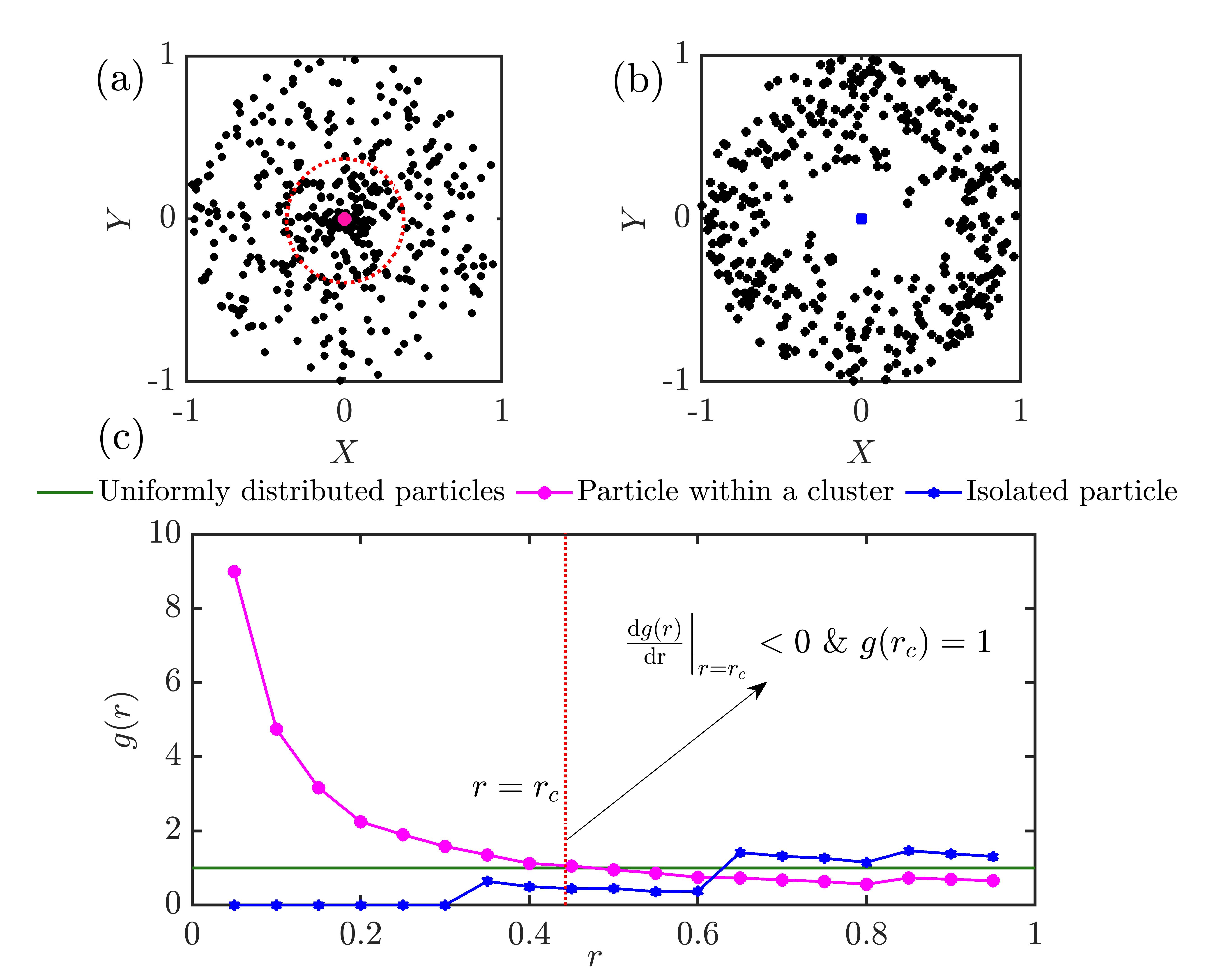
Let us consider two scenarios to illustrate the use of in our network construction, a particle that is well entrenched in a cluster (Fig. 1a), and an isolated particle where particles are sparely distributed in its vicinity (Fig. 1b). The variation of for both the particles is shown in Fig. 1c. Here, for the clustered particle, is greater than one in its vicinity and decreases in the local neighborhood along the radial direction based on the spatial distribution of particles. Particles within the radius (see Fig. 1a ) are clustered relative to the reference particle and hence are connected to the reference particle in the network. For the isolated particle (see Fig. 1b), in its vicinity and increases beyond one after a specific radial distance. From the variation of , we can infer that though there are particles in the neighborhood of the reference particle, they are not in the immediate vicinity. Hence, no connection is established with this isolated particle. Following this approach, the existence of a link between any two particles is encoded into a binary adjacency matrix () as 1 if they are connected or 0 otherwise. The links established between the particles are unweighted and undirected. Since we do not consider any self-connections, is set to 0.
Using network measures such as the degree of a node () and the local clustering coefficient (), we characterize the clustering between particles. The degree of a node () quantifies the number of connections a node has with other nodes in the network. Higher indicates the presence of many particles in the vicinity of a node. To remove the dependence on the number of particles in the flow domain, we normalize with the total number of nodes in our system. The average normalized degree (), obtained by averaging the degree across all the nodes in the network (Eq. 7), provides a global estimate on the clustering amongst particles. For studying the changes in the network structure, we use degree distribution ( vs. ), where is the probability of a randomly selected node having degree .
The local clustering coefficient () captures the inter-connectivity between the neighbours of the reference node. is a local measure useful in capturing the cluster density between the neighbours of the reference node. A particle entrenched in a densely concentrated region of a cluster will have a higher value of than a particle in a moderately concentrated region. The value of lies between 0 and 1, where 0 corresponds to an absence of links between neighbors and 1 corresponds to all the neighbors being connected to each other. For obtaining a global estimate on how densely the particles are clustered, we average the clustering coefficient () across all the nodes in the network.
Network analysis of clustering in particle-laden 2D Taylor-Green flow
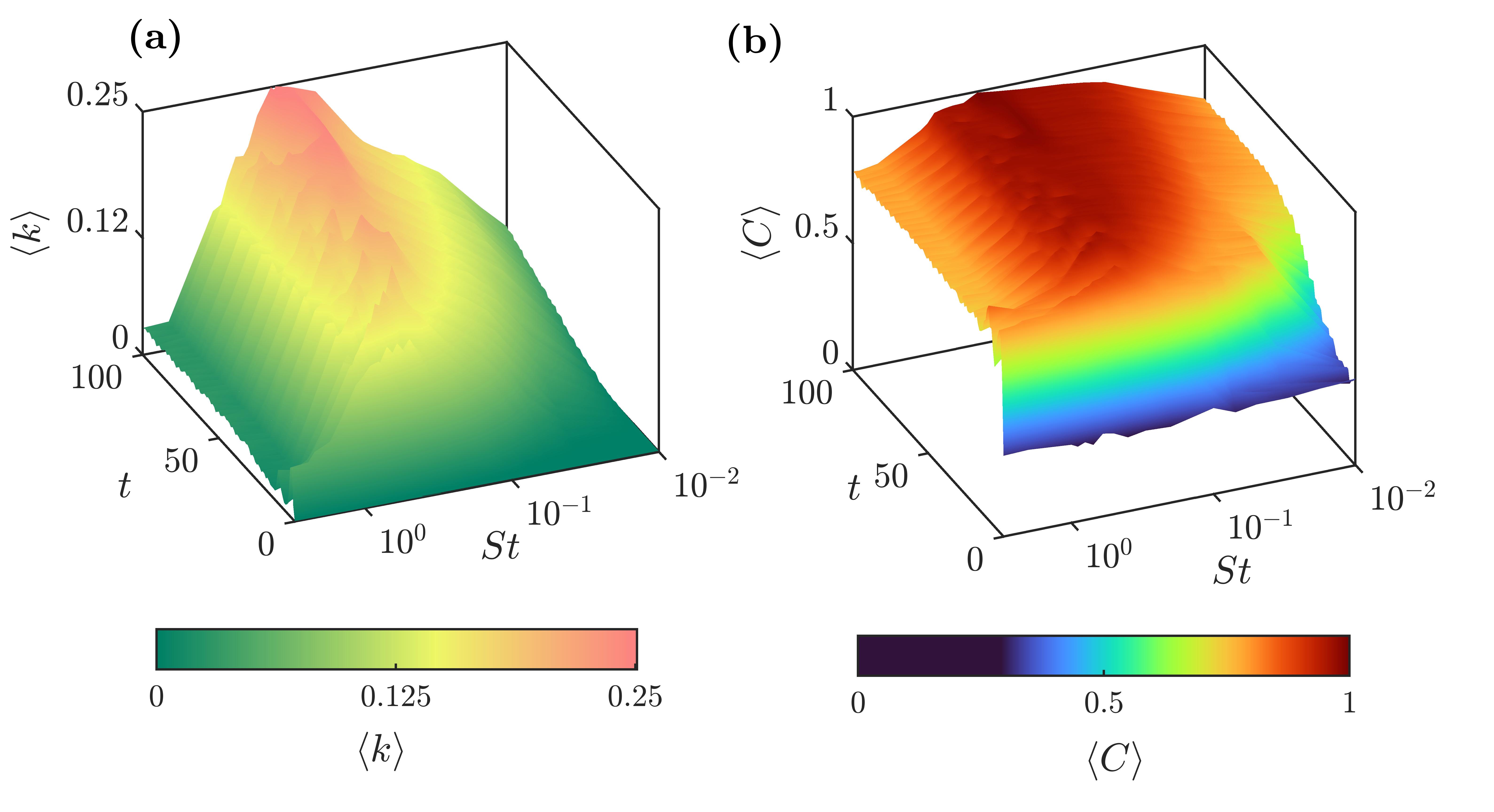
From the spatial distribution of particles at each time instant, a proximity-based complex network is constructed and characterized using and . As particles cluster in time, and of the networks increases. When particles asymptotically settle into the stagnation points, the values of and saturate at and , respectively. Weakly inertial particles () cluster slowly which is evident from the gradual increase of and (Fig. 2 and movie S1).
As we increase , the rate at which particles are centrifuged out increases (?); hence, for , both and values increase rapidly. For , all particles in the flow domain asymptotically settle into the stagnation points (movies S1 and S2). Hence, as , both and saturate at and respectively. For , a fraction of particles exhibit periodic motion without settling into the stagnation points (?) (movie S3). As we increase the , the fraction of particles exhibiting periodic motion increases. Hence, we observe a decrease in the saturated values of and for . Furthermore, as a result of the periodic motion of particles, we observe undulations in the saturated and (Fig. 2). For , all the particles exhibit periodic motion without clustering in the shear regions, which is reflected in the lower values of and . Thus, the emergence of clusters for saturates the average network measures at a high value reflecting the global clustering characteristics. These observations are illustrated and analyzed here in detail for the specific cases of , and as shown in Fig. 3- 5.
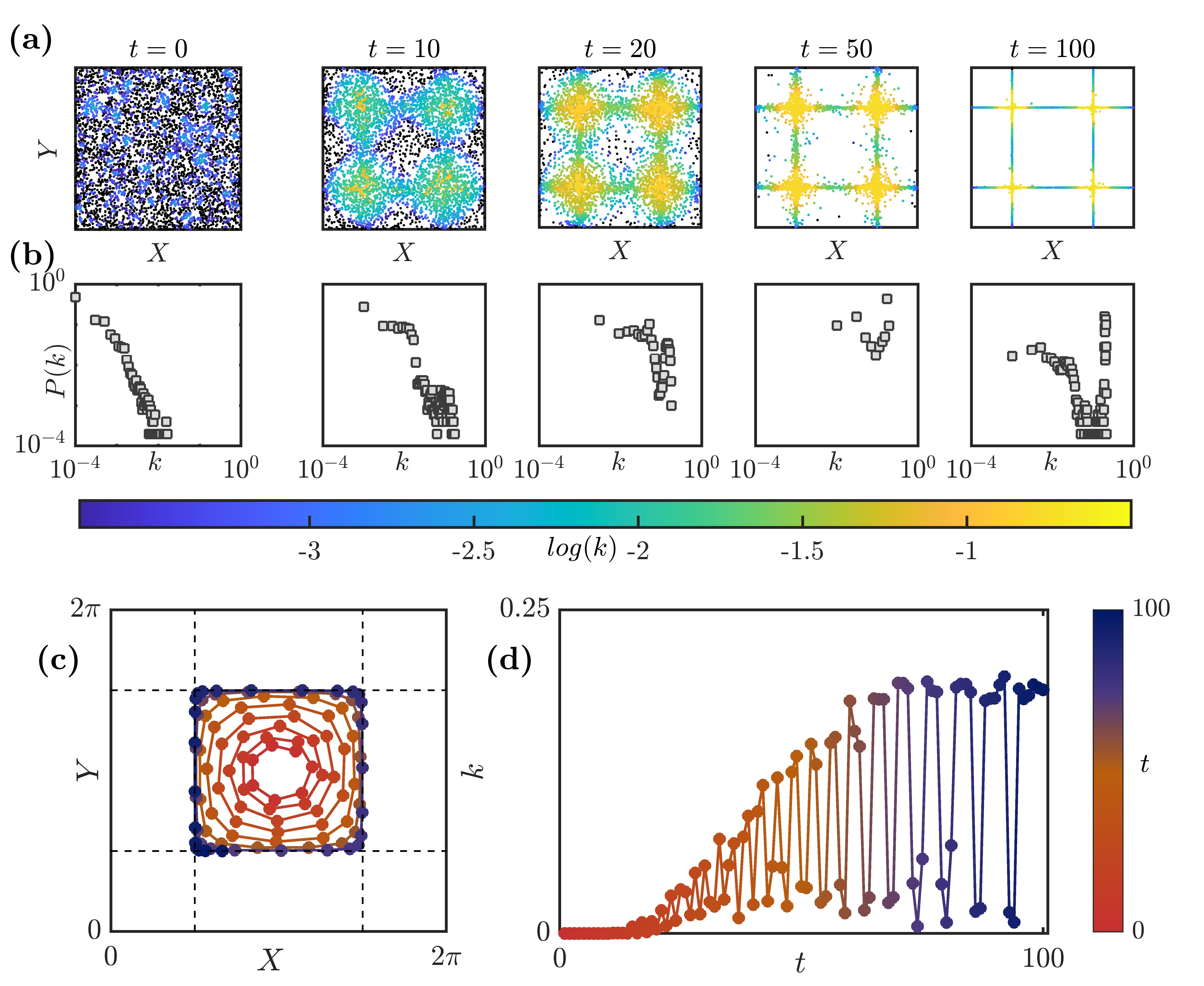
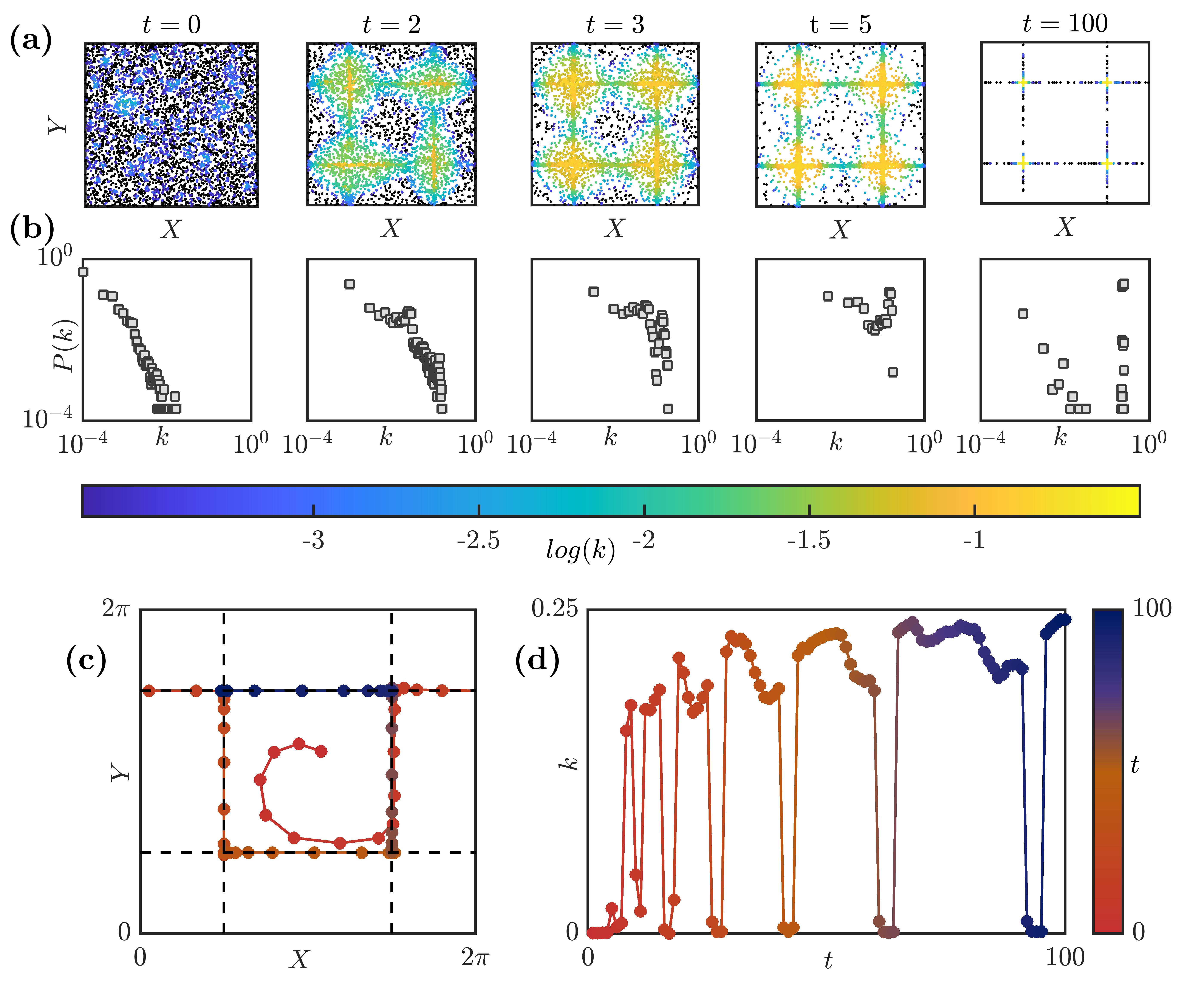
We start with a random initial distribution of particles in the flow domain (Fig. 3-5(a) at ). In the corresponding network at , most particles have a few connections () while a few nodes have more than just a few connections (). Corresponding, we observe a power law behaviour in the degree distribution for randomly distributed particles (Fig. 3-5(b) at ). The inertia of particles comes into play for , and the simulations are performed up to .
As we progress in time, particles move out of their streamlines and form prominent cluster patterns. The time at which cluster patterns become apparent differ with ; for and , patterns that resemble a cross emerge in the shear regions at and , respectively (movies S1, S2 and S3). The scatter plots in Fig. 3-5(a) show the increase in the degree of particles that start clustering in the shear region. Correspondingly, we observe a distortion of the original power-law degree distribution in Fig. 3-5(b). As particles form dense clusters, the number of particles with higher increases significantly.
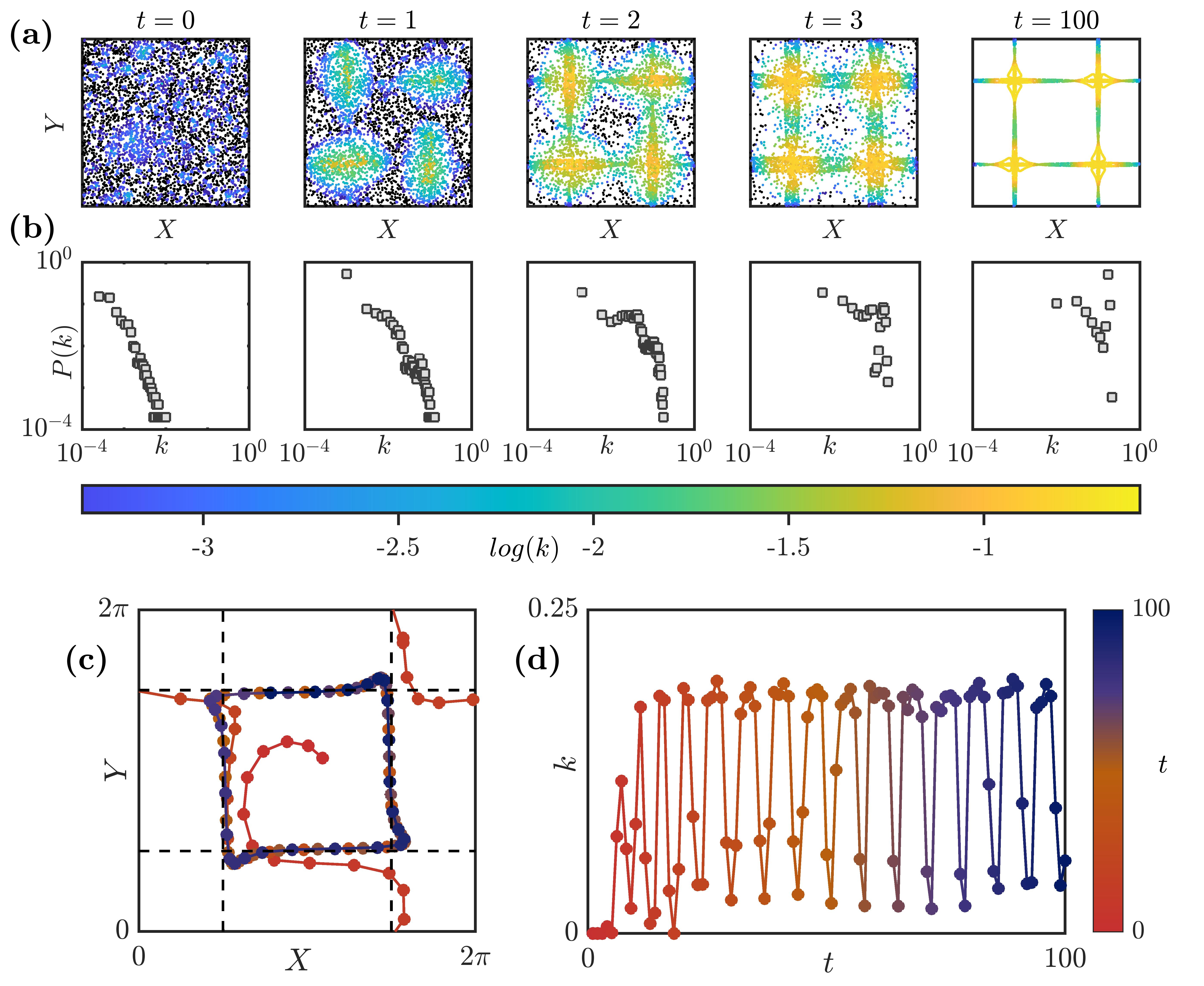
Thus, the corresponding network possesses a large fraction of nodes with higher degrees. In the degree distribution at , the particles with high correspond to the particles near the stagnation points while particles with low correspond to the few particles commuting between these stagnation points in the shear regions. Finally, at very large , for and , all particles settle into the four stagnation points, thus exhibiting a steady state clustering (movies S1 and S2).
The trajectory of a particle initiated in the vortical region is governed by its and the underlying flow field. Particles with , do not cross the separatrices in the shear regions due to their weak inertia (?, ?). Instead, the particle gets slowly centrifuged outwards and asymptotically settles into a stagnation point in the edge of the vortex (see Fig.3c ). As this particle starts nearing the stagnation point, the number of particles in its neighbourhood start to increase and hence its value increases. The oscillations in arise as the particle approaches and moves farther from stagnation points due its the centrifugal motion. The peaks and troughs in occur when a particle is nearest and farthest from the stagnation points respectively. Moreover, the frequency of the oscillations in are directly related to the frequency of the spiral motion of the particle in the vortical region.
On the other hand, a particle with initialized inside a vortical region has sufficient inertia to cross the separatrices. Thus, particles originating in different regions can interact with each other (?, ?) (evident in Fig. 4(c)). Since a particle in the vortical region is quickly centrifuged out and enters the shear region, of the particle increases sharply. The frequency of oscillation in is determined by the time the particle takes to move from one stagnation point to the other in the shear region.
Finally, for , the particle response time matches with the flow time scale. Particles are ejected very rapidly from the vortex regions and form dense clusters in the shear regions (Fig. 5(a) and movie S3). As a result, of the particle increases sharply. These particles do not asymptotically settle into the stagnation point; instead, they move in specific periodic orbits in the shear region (Fig. 5(c)). The frequency of oscillation of is clearly a function of the frequency of particle motion in its periodic orbit. The patterns formed by a collection of such particles remain consistent with time (Fig. 5(a) at ).
Clustering as a continuous phase transition
The connections between the nodes in the network increase drastically as particles organize into cluster patterns that resemble a cross. The size of the largest component is defined as the total number of nodes in the largest connected set of nodes in the network (?). Here, we draw inferences about the process of clustering in particle-laden 2D Taylor-Green flow by studying the variation of of the network, which indicates the extent of clustering amongst particles at any given time. The normalized size of the largest component () changes drastically from to over a finite time interval () characterizing a phase transition. In this study, when , the largest component is referred to as the giant component. The emergence of a giant component in the network often occurs via a phase transition (?). Here, we use as the order parameter to characterize this phase transition.
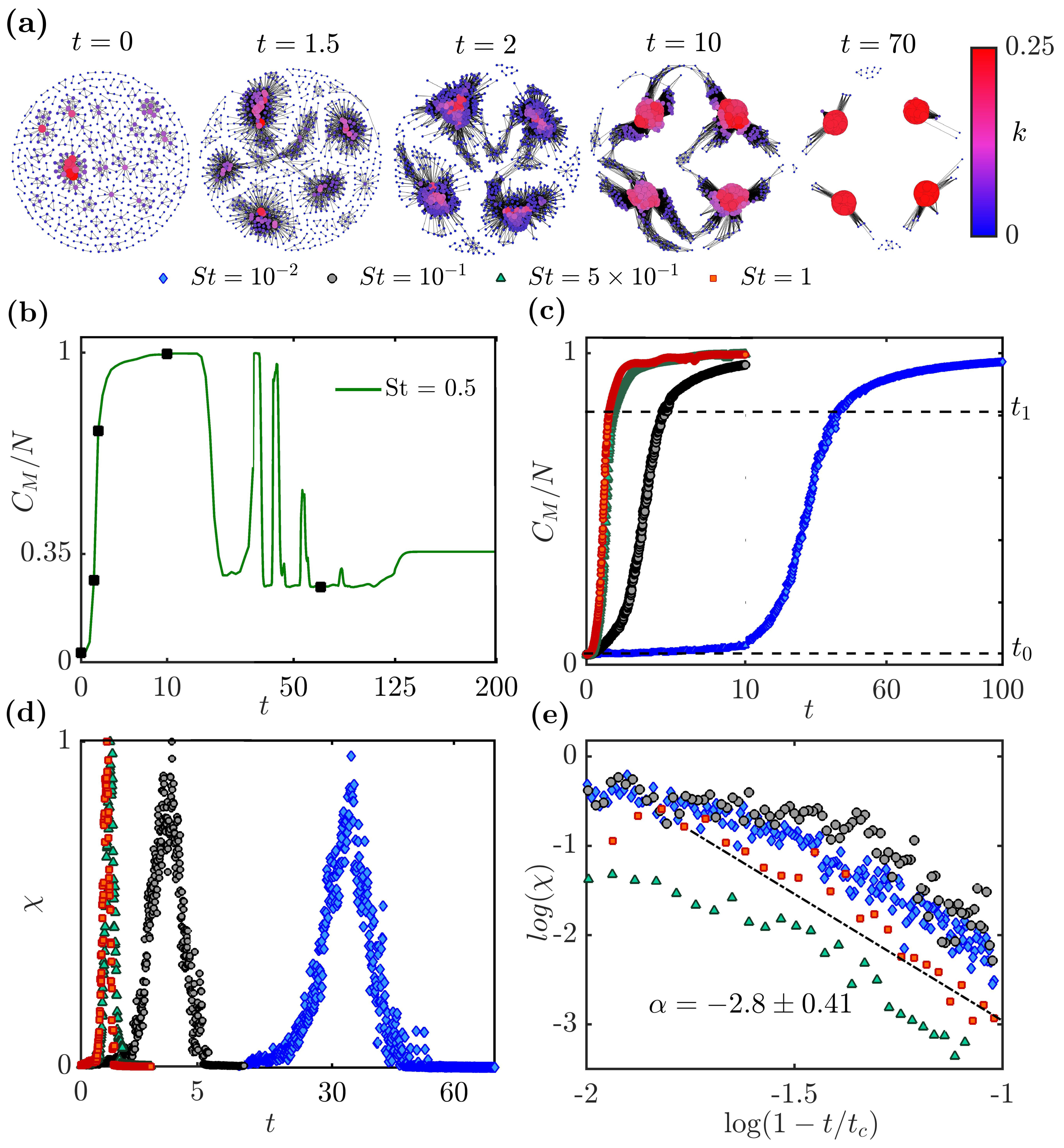
For particles with , the phase transition in the derived networks occurs around (see Fig. 6a-b) as increases rapidly in a short epoch owing to the rapid clustering of particles in the shear regions (see Fig. 4a). The results in Fig. 6 are obtained for an ensemble of realizations and for a time resolution of 0.02. The size of the giant component saturates and reaches a maximum for a significant epoch between to (see Fig. 6b). During this epoch, a significant proportion of particles commute in the shear regions between the stagnation points (see Fig. 4a). As particles asymptotically settle into the stagnation points, the number of particles commuting between stagnation points in the shear region reduces leading to the fragmentation of the network and a corresponding decrease in . Note that, the number of particles that settle asymptotically into each stagnation point is not necessarily equal after complete clustering occurs in the flow field, and thus the size of the largest cluster not necessarily tends to as (see Fig. 6b). The oscillations in occur due to the decrease in connections in the network as the number of particles commuting between stagnation points reduces.
The rate of phase transition in proximity networks is a strong function of (Fig. 6(c)). Significant variation in the observed in Fig. 6(c) occurs precisely when patterns that resemble a cross become apparent in the flow (Fig. (3-5)a). The time interval of phase transition () is determined by setting thresholds for the order parameter (). We define , where is the maximum time at which , i.e., when is a fractional power of the network size. Further, is the minimum time at which , i.e., when is a significant fraction of the network size. For the results presented in our analysis, we choose and . We observe that decreases as we increase from to (Fig. 7). Clearly, depends on the time taken for the particles to form clusters of discernible patterns in the flow.
A typical feature of phase transitions is the divergence of the variance of fluctuations of the order parameter, called susceptibility (), around the critical time when the transition occurs. Susceptibility () is defined as , where is the ensemble average operator. From Fig. 6(d), we observe that susceptibility diverges at faster rate and at lower critical times () for higher values of . Here, is identified as the time at which attains its peak value in Fig. 6(d). For lower values of , this transition occurs over a longer time interval and at higher values of when compared to that during higher values of . Shorter epochs of phase transition for particles with higher indicate the tendency of such particles to cluster rapidly. In Fig. 6(e), we plot the variation of as a function of on a log-log scale. Firstly, we note in Fig. 6(e) that the critical behavior during phase transition for various exhibits a power-law scaling around the critical time as , with critical exponent with confidence.
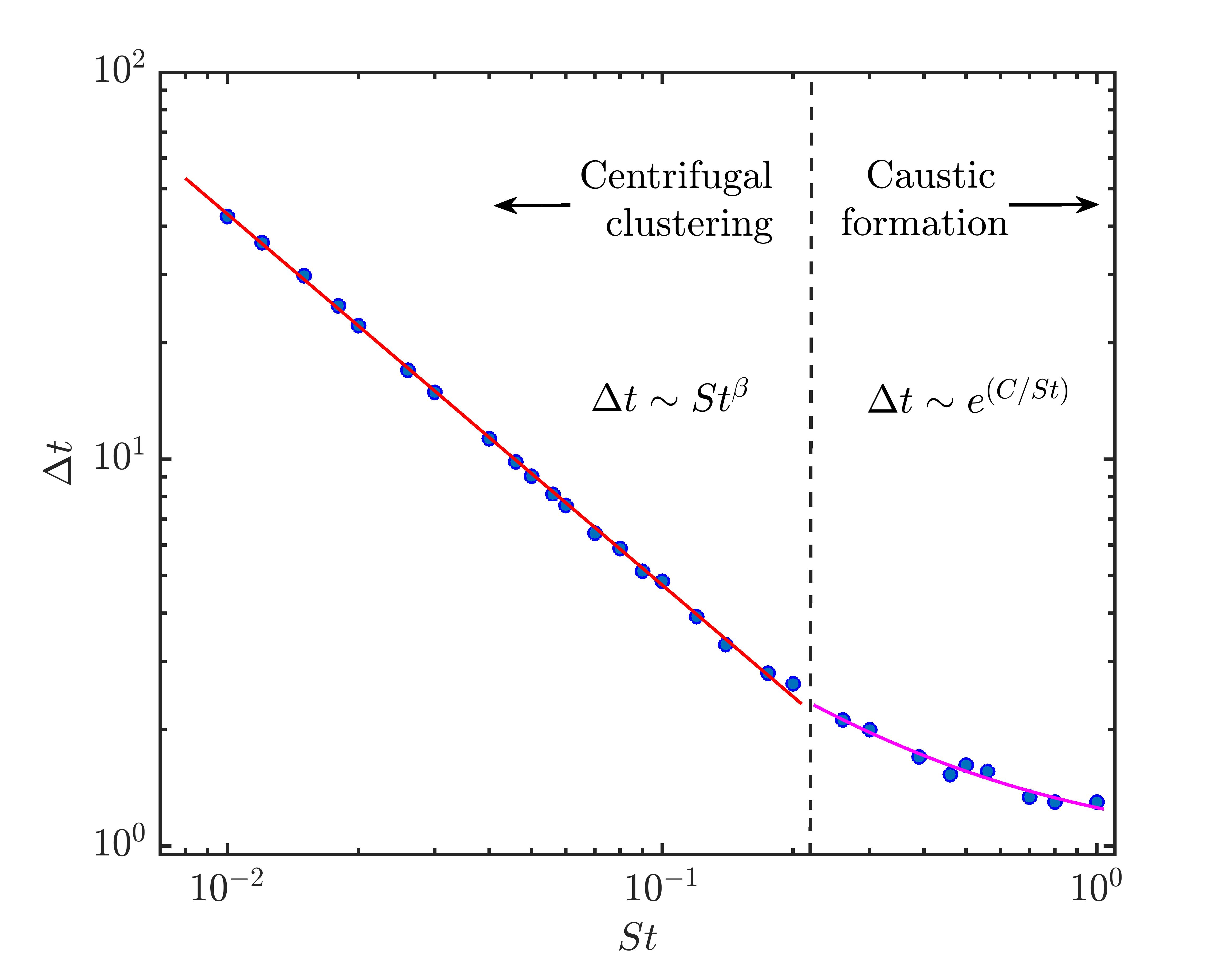
For , the particles are essentially tracer particles and do not form any spatial clusters as they follow the fluid streamlines indefinitely. Therefore, there is no phase transition observed for such particles, and thus as . For inertial particles with , the response time of particles is close to the flow timescale and the particles tend to cluster rapidly. Figure 7 shows the variation of with which clearly follows a power-law with a scaling exponent with confidence, initially for . For particles with , the phase transition time varies in the form with the constant with confidence. This deviation from power-law behaviour could possibly be due to the formation of caustics amongst the particles in this range and the variation of is consistent with the rate of caustics formation (?, ?).
DISCUSSION
We propose the use of complex networks to study the local and global dynamics in particle-laden flows. The local attributes of a network such as the degree of any individual particle captures the local clustering characteristics along its trajectory. On the other hand, the saturation of average network measures reflects the global clustering characteristics of the particles. Further, the distortion of the initial power-law degree distribution reflects the spatial inhomogeneities among particles due to cluster formation. As the connectivity of the proximity-based particle network increases, a giant component emerges in the network. Such an emergence of giant component signifies the formation of particle-clusters in the flow and this process occurs via a continuous phase transition. The network approach reveals a universal behavior of the inertial particles close to the critical time of phase transition evoked by the clustering dynamics in the flow despite the differences in . The phase transition time exhibits a power-law behaviour for and an exponential behaviour for possibly due to the formation of caustics.
MATERIALS AND METHODS
Model
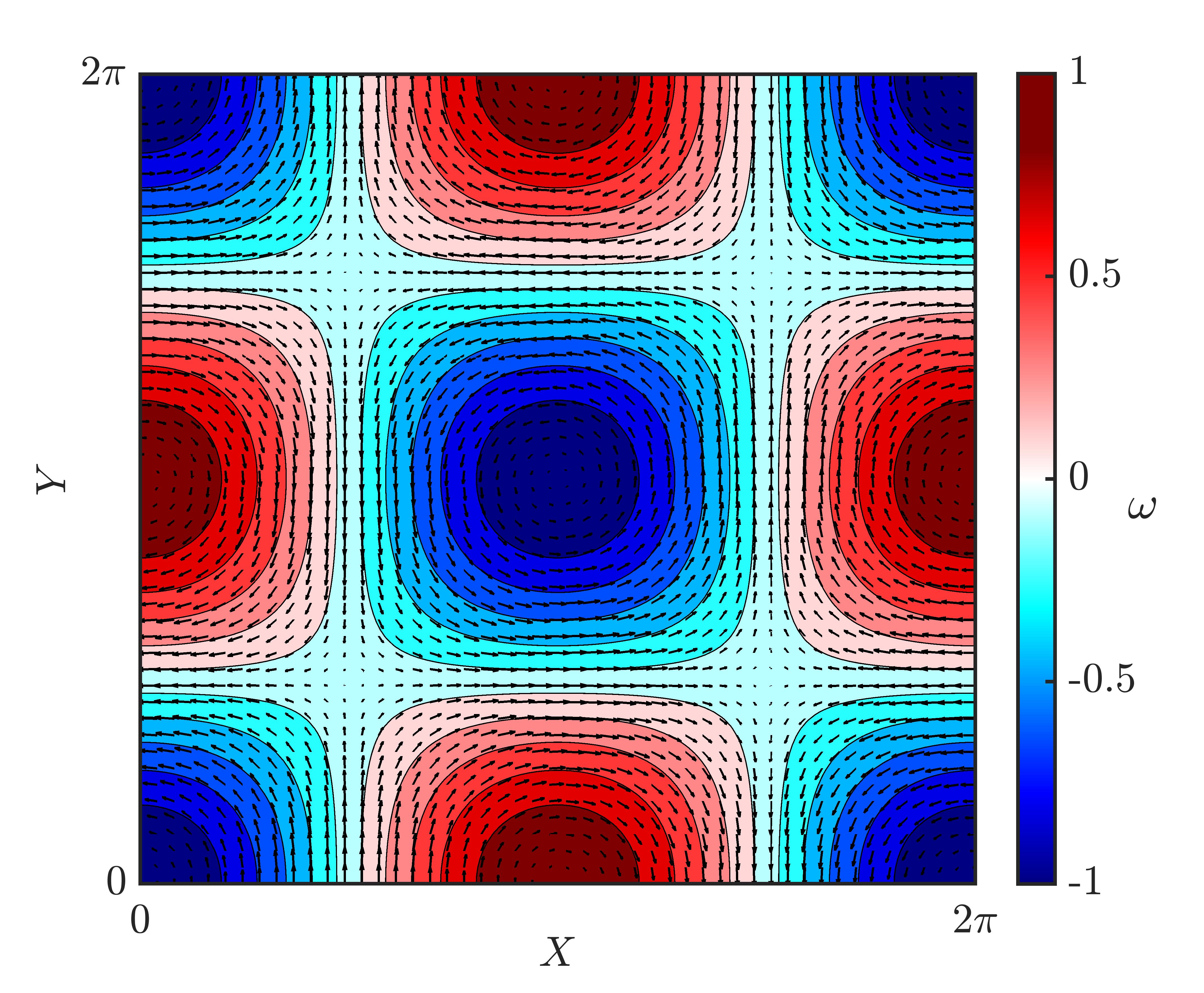
In order to understand the clustering process using complex networks, we choose the steady 2-D Taylor-Green flow (?, ?) to be our canonical flow (Fig. 8). This simple flow was chosen for our analysis as it has some of the features of turbulent flows such as coexisting regions of vorticity and shear (?, ?, ?).
The velocity profile equations for Taylor-Green flow are as follows:
| (2) |
| (3) |
In the above equation, and are the two components of fluid velocity. Here, and are the length of the flow domain and the velocity of the fluid flow. The time scale, , of the flow is calculated as . These aforementioned parameters are used to non-dimensionalize the system of equations in order to minimize the number of input parameters for initiating the simulation. The particles are modeled as point particles having a significantly higher density compared to the surrounding fluid, i.e., . Due to the high density ratio, the contributions of added mass effect, buoyancy and Basset history force were neglected (?). Therefore, following the Maxey-Riley equation (?), only the effect of Stokes drag is considered in the particle dynamics.
We considered particles in our analysis to maintain a sufficiently low volume fraction, to ensure the validity of the unidirectional coupling and to keep the computational time within reasonable limits. In unidirectional coupling, the particle motion is affected by the local fluid structures but the collective motion of the particle does not affect the fluid structures. The dimensionless form of the equations are:
| (4) |
| (5) |
Here, , and are the non-dimensional particle position, flow velocity, and particle velocity vectors, respectively. For obtaining different spatial distributions of particles, we perform the analysis for various values from to . We limit our study in the range less than , as the assumption of neglecting the added mass effect and Basset history force becomes invalid for greater than (?).
At = 0, the particles are randomly distributed across the flow domain with initial velocities identical to that of the surrounding flow velocity. Then, the particle inertia is activated. We implement a periodic boundary condition across the edges of the flow domain. The simulations are performed up to non-dimensional units of time with a time step of . The simulation results are consistent with previously reported results from the literature (?, ?, ?). Using the simulated data, we construct complex networks to study the particle clustering process.
Effect of number of particles in the flow domain
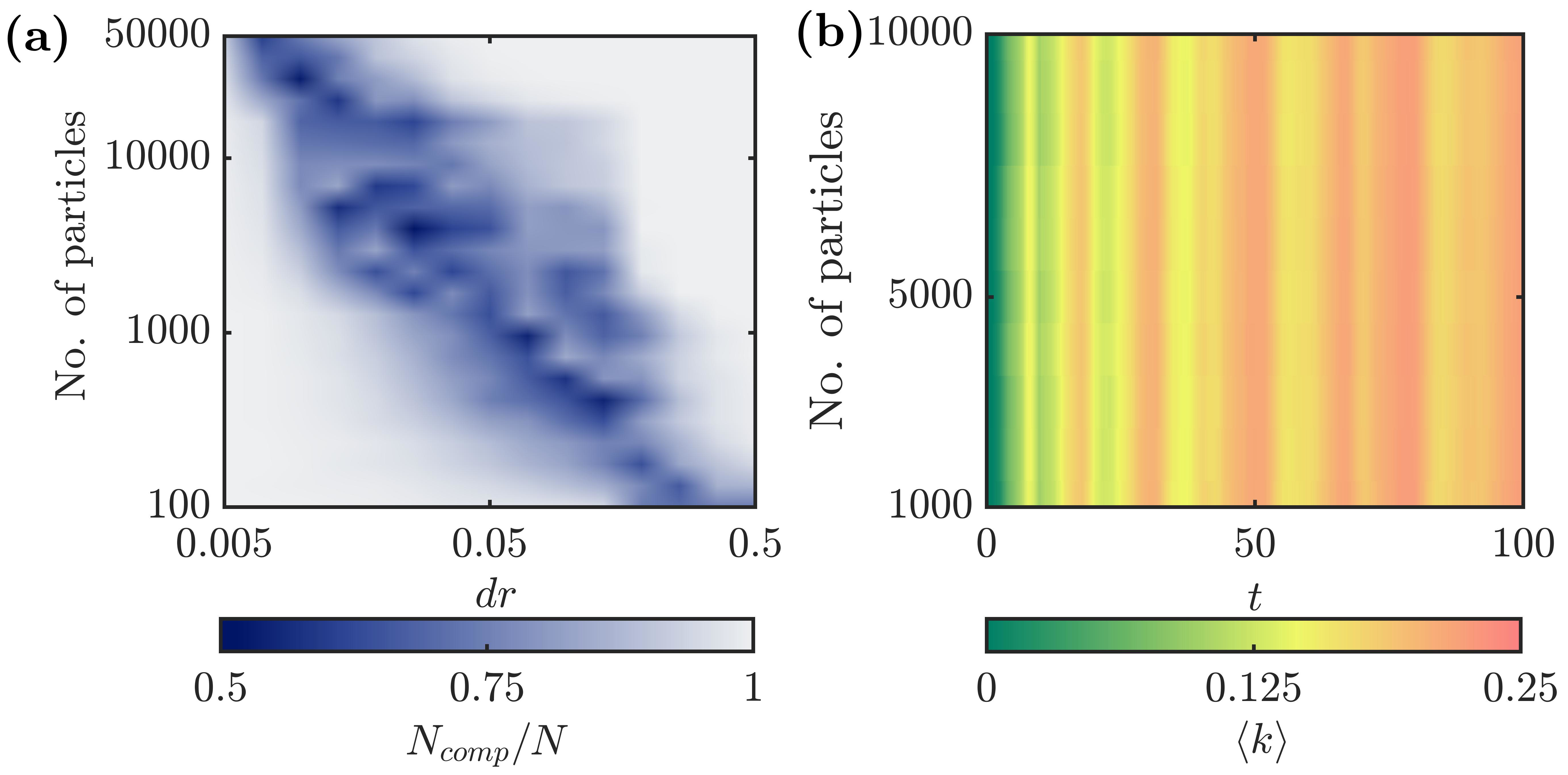
Though is defined as a continuous function, for estimating it, we need to discretize the space in the vicinity of the particle along the radial direction. Since, we construct our networks from , an optimal discretization resolution () should be selected, depending upon the number of particles in the flow domain () and the size of the flow domain (). Towards this purpose, we analyzed the variation of the normalized number of components () of the network constructed from randomly distributed particles with respect to the variation of for a fixed flow domain size (see Fig. 9). We fixed the size of the flow domain as and varied from 100 to 50000.
For a specific value of , for a small values, will have sharp peaks at the locations where particles are present and remain zero everywhere else, making it unsuitable for network construction. Hence, the conditions given in Eq. 3 will not be satisfied and the links between particles cannot be established. Thus, the network has a few connections () (see Fig. 9a). For very large , , hence becomes incapable of capturing the spatial inhomogeneities, leading to (see Fig. 9a). Between the two extremes, there are intermediate values of where reaches a minimum. We choose the where goes below unity and reaches a minimum in our study. At this resolution , the calculated is considered optimal for constructing the network and capturing the spatial inhomogeneities. When the network is constructed using this optimal , the degree distribution of the network at =0 corresponding to randomly distributed particles follows a power-law behavior. To verify this, we studied the variation of with time for particles by varying from 1000 to 10000 (see Fig. 9b). The variation of does not depend to the choice of and therefore indicative of the robustness of this method in analyzing the clustering characteristics in particle-laden flows.
Network measures
The degree of a node can be expressed in terms of the adjacency matrix as follows,
| (6) |
The average degree () is calculate as
| (7) |
The local clustering coefficient ()
| (8) |
where is the total number of links between the neighbors of node i. The average clustering () is calculate as
| (9) |
Supplementary materials
movie S1. Motion of particles in the flow domain with the color representing its corresponding degree in log-scale.
movie S2. Motion of particles in the flow domain with the color representing its corresponding degree in log-scale.
movie S3. Motion of particles in the flow domain with the color representing its corresponding degree in log-scale.
References
- 1. R. A. Shaw, Particle-turbulence interactions in atmospheric clouds, Ann. Rev. Fluid Mech. 35, 183 (2003).
- 2. S. Sahu, Y. Hardalupas, A. Taylor, Interaction of droplet dispersion and evaporation in a polydispersed spray, J. Fluid Mech. 846, 37 (2018).
- 3. R. Mittal, R. Ni, J.-H. Seo, The flow physics of covid-19, J. Fluid Mech. 894 (2020).
- 4. T. Haszpra, T. Tél, Volcanic ash in the free atmosphere: A dynamical systems approach, J. Phys.: Conf. Ser. (IOP Publishing, 2011), vol. 333, p. 012008.
- 5. N. Smith, G. Nathan, D. Zhang, D. Nobes, The significance of particle clustering in pulverized coal flames, Proc. Comb. Inst. 29, 797 (2002).
- 6. E. Bodenschatz, S. P. Malinowski, R. A. Shaw, F. Stratmann, Can we understand clouds without turbulence?, Science 327, 970 (2010).
- 7. W. W. Grabowski, L.-P. Wang, Growth of cloud droplets in a turbulent environment, Ann. Rev. fluid mech. 45, 293 (2013).
- 8. A. Pumir, M. Wilkinson, Collisional aggregation due to turbulence, Ann. Rev. Cond. Matt. Phys. 7, 141 (2016).
- 9. L. Sabban, R. van Hout, Measurements of pollen grain dispersal in still air and stationary, near homogeneous, isotropic turbulence, J. Aerosol sci. 42, 867 (2011).
- 10. H. Chiu, T. Liu, Group combustion of liquid droplets, Comb. Sci.Tech. 17, 127 (1977).
- 11. C. Crowe, M. Sommerfeld, Y. Tsuji, Multiphase Flows with Particles and Droplets (CRC Press, New York, 1998).
- 12. K. D. Squires, J. K. Eaton, Preferential concentration of particles by turbulence, Phys. Fluids A 3, 1169 (1991).
- 13. J. K. Eaton, J. Fessler, Preferential concentration of particles by turbulence, Int. J. Multiphase Flow 20, 169 (1994).
- 14. L.-P. Wang, M. R. Maxey, Settling velocity and concentration distribution of heavy particles in homogeneous isotropic turbulence, J. Fluid Mech. 256, 27 (1993).
- 15. J. Chun, D. L. Koch, S. L. Rani, A. Ahluwalia, L. R. Collins, Clustering of aerosol particles in isotropic turbulence, J. Fluid Mech. 536, 219 (2005).
- 16. A. Aliseda, A. Cartellier, F. Hainaux, J. C. Lasheras, Effect of preferential concentration on the settling velocity of heavy particles in homogeneous isotropic turbulence, J. Fluid Mech. 468, 77 (2002).
- 17. E. W. Saw, R. A. Shaw, S. Ayyalasomayajula, P. Y. Chuang, A. Gylfason, Inertial clustering of particles in high-reynolds-number turbulence, Phys. Rev. Lett. 100, 214501 (2008).
- 18. S. Sundaram, L. R. Collins, Collision statistics in an isotropic particle-laden turbulent suspension. part 1. direct numerical simulations, J. Fluid Mech. 335, 75 (1997).
- 19. H. Lian, G. Charalampous, Y. Hardalupas, Preferential concentration of poly-dispersed droplets in stationary isotropic turbulence, Experiments in fluids 54, 1 (2013).
- 20. R. Monchaux, M. Bourgoin, A. Cartellier, Preferential concentration of heavy particles: a voronoï analysis, Phys. Fluids 22, 103304 (2010).
- 21. Y. Tagawa, et al., Three-dimensional lagrangian voronoï analysis for clustering of particles and bubbles in turbulence, J. Fluid Mech. 693, 201 (2012).
- 22. Z.-K. Gao, M. Small, J. Kurths, Complex network analysis of time series, Europhys. Lett. 116, 50001 (2017).
- 23. G. Iacobello, L. Ridolfi, S. Scarsoglio, A review on turbulent and vortical flow analyses via complex networks, Physica A p. 125476 (2020).
- 24. E. Bormashenko, A. A. Fedorets, M. Frenkel, L. A. Dombrovsky, M. Nosonovsky, Clustering and self-organization in small-scale natural and artificial systems, Philos. Trans. R. Soc. A 378, 20190443 (2020).
- 25. L. Brandt, F. Coletti, Particle-laden turbulence: Progress and perspectives, Ann. Rev. Fluid Mech. 54 (2021).
- 26. A.-L. Barabási, M. Pósfai, Network science (Cambridge University Press, Cambridge, 2016).
- 27. S. Scarsoglio, F. Laio, L. Ridolfi, Climate dynamics: a network-based approach for the analysis of global precipitation, PLoS One 8, e71129 (2013).
- 28. E. Ser-Giacomi, V. Rossi, C. López, E. Hernández-García, Flow networks: A characterization of geophysical fluid transport, Chaos 25, 036404 (2015).
- 29. G. Iacobello, S. Scarsoglio, J. Kuerten, L. Ridolfi, Spatial characterization of turbulent channel flow via complex networks, Phys. Rev. E 98, 013107 (2018).
- 30. K. Taira, A. G. Nair, S. L. Brunton, Network structure of two-dimensional decaying isotropic turbulence, J. Fluid Mech. 795 (2016).
- 31. V. R. Unni, et al., On the emergence of critical regions at the onset of thermoacoustic instability in a turbulent combustor, Chaos 28, 063125 (2018).
- 32. G. I. Taylor, A. E. Green, Mechanism of the production of small eddies from large ones, Proc. Royal Soc. London. Series A-Math. Phys. Sci. 158, 499 (1937).
- 33. M. R. Maxey, J. J. Riley, Equation of motion for a small rigid sphere in a nonuniform flow, Phys. Fluids 26, 883 (1983).
- 34. M. Maxey, The motion of small spherical particles in a cellular flow field, Phys. Fluids 30, 1915 (1987).
- 35. S. N. Dorogovtsev, A. V. Goltsev, J. F. Mendes, Critical phenomena in complex networks, Rev. Mod. Phys. 80, 1275 (2008).
- 36. D. Achlioptas, R. M. D’Souza, J. Spencer, Explosive percolation in random networks, Science 323, 1453 (2009).
- 37. D. Lee, B. Kahng, Y. Cho, K.-I. Goh, D.-S. Lee, Recent advances of percolation theory in complex networks, J. Kor. Phys. Soc. 73, 152 (2018).
- 38. M. Elliott, B. Golub, M. O. Jackson, Financial networks and contagion, Am. Econ. Rev. 104, 3115 (2014).
- 39. P. Gai, S. Kapadia, Contagion in financial networks, Proc. R. Soc. A 466, 2401 (2010).
- 40. M. Tang, L. Liu, Z. Liu, Influence of dynamical condensation on epidemic spreading in scale-free networks, Phys. Rev. E 79, 016108 (2009).
- 41. S. Tandon, R. I. Sujith, Condensation in the phase space and network topology during transition from chaos to order in turbulent thermoacoustic systems, Chaos 31, 043126 (2021).
- 42. P. Erdos, A. Rényi, On the evolution of random graphs, Publ. Math. Inst. Hung. Acad. Sci 5, 17 (1960).
- 43. R. M. D’Souza, J. Gómez-Gardenes, J. Nagler, A. Arenas, Explosive phenomena in complex networks, Adv. Phys. 68, 123 (2019).
- 44. S. Ravichandran, R. Govindarajan, Caustics and clustering in the vicinity of a vortex, Phys. Fluids 27, 033305 (2015).
- 45. A. V. Nath, A. Roy, R. Govindarajan, S. Ravichandran, Transport of condensing droplets in taylor-green vortex flow in the presence of thermal noise, https://arxiv.org/abs/2111.04102 (2021).
- 46. D. Healy, J. Young, Full lagrangian methods for calculating particle concentration fields in dilute gas-particle flows, Proc. R. Soc. A 461, 2197 (2005).
- 47. D. Larremore, Find network components, https://www.mathworks.com/matlabcentral/fileexchange/42040-find-network-components. MATLAB Central File Exchange. Retrieved November 22, 2021.
- 48. R. Albert, A.-L. Barabási, Statistical mechanics of complex networks, Rev. Mod. Phys. 74, 47 (2002).
- 49. T. M. Fruchterman, E. M. Reingold, Graph drawing by force-directed placement, Software: Practice and experience 21, 1129 (1991).
- 50. M. Bastian, S. Heymann, M. Jacomy, Gephi: an open source software for exploring and manipulating networks, Third international AAAI conference on weblogs and social media (2009).
- 51. O. Samant, J. K. Alageshan, S. Sharma, A. Kuley, Dynamic mode decomposition of inertial particle caustics in taylor-green flow, Scientific Reports 11, 1 (2021).
- 52. M. Cencini, et al., Dynamics and statistics of heavy particles in turbulent flows, J. Turbul. p. N36 (2006).
- 53. A. Crisanti, M. Falcioni, A. Provenzale, A. Vulpiani, Passive advection of particles denser than the surrounding fluid, Phys. Lett. A 150, 79 (1990).
Acknowledgments
Funding: We gratefully acknowledge the funding from J. C. Bose fellowship (JCB/2018/000034/SSC) from the Science and Engineering Research Board (SERB) of the Department of Science and Technology (DST), Government of India.
Author contributions:
K. S. V.: conceptualization, developed source code, simulations, analysis, writing and editing original draft; S. T.: conceptualization, validation and analysis of phase transition, writing and editing original draft; P. K.: conceptualization, supervision, writing and editing draft; R. I. S.: conceptualization, supervision, writing and editing draft;
Declaration of competing interests
The authors declare that they have no competing interests.
Data and materials availability
All data needed to evaluate the conclusions are present in the paper and the supplementary Materials. Additional data related to this paper will be available upon request to the authors.