CM elliptic curves: volcanoes, reality and applications, Part II
Abstract.
Let be positive integers, and let be the discriminant of an order in an imaginary quadratic field . When , the first author determined the fiber of the morphism over the closed point corresponding to and showed that all fibers of the map over were connected. [Cl22a]. In the present work we complement the work of [Cl22a] by addressing the most difficult cases . These works provide all the information needed to compute, for each positive integer , all subgroups of , where is a number field of degree and is an elliptic curve with complex multiplication.
1. Introduction
1.1. Main Results
This paper is a direct continuation of [Cl22a], which determined the -CM locus on the modular
curves for the discriminant of an order in an imaginary quadratic field different from or . This work also gave a completely explicit description of the primitive residue fields of -CM closed points: i.e., the residue fields of -CM points for which there is no -CM point such that embeds into as a proper subfield. Finally, the work [Cl22a] also gave an inertness result for the fibers of over -CM points on , which yields a complete description
of the multiset of degrees of -CM closed points on . Using only the knowledge of the degrees of primitive residue fields of -CM points on yields the corresponding knowledge of degrees of primitive residue fields of -CM
points on , which is precisely what is needed in order to classify torsion subgroups of -CM elliptic curves
over number fields of any fixed degree.
In the present work we treat the excluded fields and . If
and , then for all we determine the -CM locus on and explicitly determine
all primitive residue fields of -CM points on . Finally, we show that the fibers of over -CM points are connected.111The difference between “inertness” and “connectedness” is that the latter
allows ramification. The map can only ramify over , and .
Taken together, the works [Cl22a] and the present work give a complete description of torsion subgroups of CM elliptic curves
over number fields. In particular, we get an algorithm that takes as input a positive integer and outputs the complete,
finite list of groups isomorphic to where is a number field of degree and is a CM elliptic curve, conditionally on knowing the finite list of imaginary quadratic orders of class number properly dividing . With current knowledge about class numbers, this allows us to enumerate CM torsion in number field degree . If we are willing to assume the Generalized
Riemann Hypothesis (GRH), then by [LLS15, Cor. 1.3] we can enumerate CM torsion in number field degree .
This enumeration will appear in a future work.
1.2. Review of the case
Let us outline the proof of the computation of the fiber of over the closed -CM point on given in [Cl22a] so that we can see what must be modified to treat the case.
Step 1: We handle the case for a prime power .
Step 1a: The -power isogeny graph corresponding to a -CM elliptic curve with (where ) has the structure of an
-isogeny volcano. This is an infinite graph that is very close to being a rooted tree and with vertex set stratified into levels indexed by ; the set of vertices at level corresponds to the set of -invariants of -CM elliptic curves, which is a torsor under , the Picard group of the imaginary quadratic order of
discriminant .
Cyclic -isogenies with -CM source elliptic curve correspond to paths of length in this volcano with initial
vertex at level . From this it is easy to see that if is such an isogeny and if the target elliptic curve has level ,
then over the field of moduli of is the ring class field , which is equal to . It follows that
Step 1b: Thus the field of moduli of is determined when contains : this happens if and only if has no real embedding ( and are “not coreal”). Otherwise we are left to decide whether is or . Both the coreality question and the dichotomy between the two possible fields can
be answered in terms of the natural action of complex conjugation on the -isogeny volcano. Determining the explicit action of
on the -isogeny volcano is one of the main contributions of [Cl22a]. In the end, depending upon whether or not the path is fixed under complex conjugation or not,222Since closed points on correspond
to certain equivalence classes of paths, the actual answer is slightly more complicated than this but can still be determined from the action of
complex conjugation on the isogeny graph. we get that is isomorphic to –
that is, isomorphic to a rational ring class field – the field obtained by adjoining to the -invariant of an elliptic curve with CM by the imaginary quadratic
order of discriminant – or to the ring class field – which is obtained
by adjoining to the same -invariant.
Step 2: We pass from the prime power case to the case .
Step 2a: For any closed point on the -line , if , let
be the fiber of over , and for let be the fiber of
over . Then we show that is the fiber product of over . Since each is the spectrum of a
finite product of number fields, each isomorphic to either a rational ring class field or a ring class field, is determined by
in terms of tensor products of these rational ring class fields and ring class fields.
Step 2b: Letting be the rational ring class field of conductor , we show that
| (1) |
and
| (2) |
These identities allow us to write down explicitly as a product of number fields.
Step 3: Lifting a point on induced by an isogeny to a point involves
scalarizing the modulo Galois representation on , with the effect that is obtained from by adjoining
the projective -torsion field . This uses that because , the projective -torsion field
is independent of the choice of -rational model. Indeed, for all , if is a -CM elliptic curve,
we find that .
1.3. The case
When and is a -CM elliptic curve, then for certain some
of the above steps still hold. However, when , none of the above arguments hold as stated. While some of the change are routine, in several places
we have to make arguments that are significantly more intricate than those of [Cl22a]. Let us describe the modifications:
Step 1a: When , is a prime numer, and , then again the -power
isogeny graph of a -CM elliptic curve is an -volcano. When , the -power
isogeny graph is no longer an -volcano. This is in fact the least of our worries, as the deviation from “volcanoness” is minor and had already been well understood: the differences involve multiple edges descending from the surface and in subtleties involving orientations of edges which necessitate more care in the notion of a “nonbacktracking path.” The structural information we need is found, for instance, in [Su12].
Step 1b: When , there is in fact no canonical action of complex conjugation on the
-isogeny graph. To define the action of complex conjugation on isogenies, we need a priori a chosen -model
on the elliptic curve. Every real elliptic curve has precisely two nonisomorphic -models. When these two -models
are quadratic twists of each other, so the action of on finite subgroup schemes of is independent of the choice
of -model. However, when this is no longer the case.
It turns out that when , in most cases we can define a noncanonical action of
on the -isogeny graph that allows us to determine fields of modulo of -CM points on in terms of real and complex paths, as in [Cl22a]. But there are two cases in which we need to pass from this isogeny graph to a certain double cover and
define an action of on that. By looking carefully on how surface edges change the -structure of a -CM elliptic
curve we are able to carry out the analysis as in [Cl22a].
Step 2a: The fiber product result referred to above [Cl22a, Prop. 3.5] is false when : the modular curve
is a desingularization of the fiber product of the morphisms . For lack of this scheme-theoretic result we need other techniques to compute the composite level fibers. We make use of the Atkin-Lehner involution to reduce to either the case
or the case when both the source and target are -CM, in which case we have a proper isogeny in the sense of
[Cl22a, §3.4] and we can reason via -ideals.
Step 2b: When , equations (1) and (2) hold for certain pairs
and fail for others: in general the compositum is a proper subfield of ; and the same holds
for rational ring class fields and . In §2 we use class field theory to show that it is still the case that and are linearly disjoint over and to determine the index of in ; we do the same for rational ring class fields; and again we calculate tensor products of rational ring class fields and ring class fields. This calculation is relatively straightforward, but
the difference in the answer causes complications related to Step 2a: when , if are coprime positive integers,
to show that the residue field of a point contains e.g. a ring class field , it suffices to show
that it contains each of and . When , we cannot argue in this way. Instead our method is to
find a rationally isogenous elliptic curve with CM conductor divisible by .
Step 3: When , the projective -torsion field of a -CM elliptic curve may depend upon the model. Nevertheless we compute the residue field for any -CM point (this amounts to computing
the minimal possible projective -torsion field as we range over models). Using this and the maps and , we can bootstrap from to , with some care: the case
behaves exceptionally to all the rest.
1.4. The CM fibers of are connected
In [Cl22a, Thm. 1.2], the first author showed an especially close relationship between points on and points on for points which do not have CM by . In particular, this theorem states that the fiber of the map is inert over any point which does not have CM by one of these two discriminants. This has the important consequence that determining the degrees of closed -CM points on and on are equivalent problems. The following theorem generalizes this result to include points with and -CM.
Theorem 1.1.
Let , and suppose that is a -CM point. Let denote the natural morphism.
-
(i)
If or if , then is inert over .
-
(ii)
Suppose that and .
-
(a)
If is a ramified point of the map or if , then is inert over .
-
(b)
Otherwise, i.e., if and is an elliptic point on , then we have
for the ramification index and residual degree of .
-
(a)
In particular, in all cases we have that the fiber of over consists of a single point.
Proof.
For the proof, we first recall some basic relevant facts: for the map is an isomorphism. For it is a -Galois covering, hence has degree . All points on not above are unramified. For the curve (and hence ) has no elliptic points of periods or , from which it follows that all points over are ramified with ramification index or . The curve has a single elliptic point of period over , while the curve has a single elliptic point of period over . (One can see these claims regarding elliptic points and ramification from elementary arguments involving congruence subgroups, in fact this is [DS05, Exc. 2.3.7]).
For the claim is [Cl22a, Thm 1.2], so suppose that . For , the point must be non-elliptic (i.e., is a ramified point of the map ). We can see this, for instance, via our analysis of paths on for any prime ; in all cases we find that any pair of independent isogenies for must include at least one with a corresponding path in which descends, and hence any or -CM point on , and hence on for , must be non-elliptic. In this case we then have that a pair inducing is well-defined up to quadratic twist, as all models for are defined over . For this reason, the same argument involving the modulo -Galois representation given in [Cl22a, Thm 1.2] applies. Similarly, this argument applies in case if is a ramified point of the map .
We now assume that is an elliptic -CM point on with . If , then is an isomorphism, so the claim is trivial. If , then because there is a single elliptic point on it follows that it must comprise the entire fiber above , giving the inertness claim. Assuming now that , we know that is elliptic while every point in is ramified with respect to the map , giving the claimed ramification index. Note that it follows that the residual degree is at most the claimed residual degree in each case.
To provide the lower bound on the residual degree, we need only modify the argument of the case slightly in a predictable way. If , then a pair inducing is well-defined up to quartic twist. Letting denote the quotient map, by tracking that action of Galois on a generator of we get a well-defined reduced mod Galois representation
which is independent of the chosen model and surjective (see [BC20a, §1.3]). As the set is stable under the action of for , we then must have
giving the result for . For , exchanging “quartic” for “cubic” and for results in the required divisibility .
∎
Remark 1.2.
The with case of Theorem 1.1 is used explicitly in [CGPS22] to transfer from knowledge of the least degree of a -CM point on , which is computed in [BC20b], to knowledge of the least degree of a -CM point on . A shadow of Theorem 1.1 is also seen in the referenced study in the case. A positive integer is of Type I or Type II, using the terminology of [CGPS22], if has an elliptic point of order or , respectively. If is of type I, then there is a single primitive degree among all elliptic points on which is the least degree of a -CM point on . In this case, the single point lying above any elliptic -CM point on provides the least degree of a -CM point on (and the analogous statements hold for Type II and ).
2. Composita of Ring Class Fields and of Rational Ring Class Fields
Let be an imaginary quadratic field, of discriminant . We put
Let be a -order in . For , there is a unique -order in with and then is the conductor ideal [Cl22a, §2.1]. We denote by the ring class field of [Cl22a, §2.3]. If , then we have
We recall from [Cx89, Cor. 7.24] the formula
| (3) |
As in [Cl22a, §2.6], we also define the rational ring class field
In [Cl22a, §2] we studied composita of ring class fields and of rational ring class fields (with a fixed imaginary quadratic field
, in both cases) when . The results were quite clean: for , the fields
and are linearly disjoint over and we have
[Cl22a, Prop. 2.2] and the same holds with each replaced by [Cl22a, Prop. 2.10a)].
Here we treat .
Proposition 2.1.
Let be a quadratic field with , let , and put
-
a)
Suppose that . Then:
-
b)
If the order of discriminant has class number , then we have
-
c)
Let be pairwise relatively prime, and further assume that:
If , then no lies in ; and
If , then no lies in .
Then: -
d)
In all cases we have that and are linearly disjoint over , and thus .
Proof.
We will use the classical description of ring class groups and ring class fields, with notation as in [Cx89, §7]. For , let be the group of fractional -ideals prime to and let be the subgroup of principal fractional ideals generated by an element such that for some with . By class field theory, we have if and only if
Clearly in all cases we have
a) Suppose and , so the units of are . Let . We may choose such that
and then there is such that
If , then the argument of Case 1 works to show that . After replacing with if necessary, the other case to consider is that
If this holds then
which is manifestly false.
Suppose and , so the units of are , ,
where . As above, we may suppose that and
is congruent modulo to either or to . We then get
which is again manifestly false.
b) This is a trivial case, listed for completeness: if the order of discriminant has class number
then (and conversely), so .333This gives rise to cases in
in which : e.g. when we have but .
c) We claim that the extensions are mutually linearly disjoint over : that is,
Since everything in sight is Galois, it is enough to check that . But the conductor of divides and the conductor of divides , so the conductor of their intersection is the unit ideal, so the intersection is contained in the Hilbert class field , hence is equal to . From this it follows that
and the latter expression may be evaluated using (3).
d) It is immediate that .
The case is easy: then has conductor dividing and , so its conductor is the unit
ideal, so is contained in the Hilbert class field of , which is the ring class field .
Henceforth we suppose that , and thus by part a) we have . We claim the formula
First we observe that this formula holds for any multiplicative function . If we had then the function would be multiplicative. Instead we have , in which case is a constant multiple of a multiplicative function except for its value at . This justifies the claim. The claim can be rewritten as
so and are linearly disjoint over , and thus . ∎
Proposition 2.2.
Let be a quadratic field with . Let , and put , . Let
this is the set of imaginary quadratic disciminants with fundamental discriminant and class number . Let
-
a)
The fields and are linearly disjoint over :
-
b)
If , then we have:
and
-
c)
If and , then we have
and
-
d)
Let be elements of that are pairwise relatively prime. Then is a subfield of of index , and moreover
Finally, if , then
Proof.
a) As in the proof of [Cl22a, Prop. 2.10], this follows from the fact that and are
linearly disjoint over .
b) If , then , and all the statements follow easily.
c) Using part a) and Proposition 2.1a), we get
so . The other two statements of part c) follow easily.
d) Again it follows from Proposition 2.1 that the field extensions are mutually linearly disjoint
over . So
The other two statements of part d) follow easily. ∎
3. The Isogeny Graph
3.1. Defining the graph
Let be an imaginary quadratic field, and let be a prime number. There is a directed multigraph as follows: the vertex set of is the set of -invariants of K-CM elliptic curves, i.e., -invariants of complex elliptic curves with endomorphism ring an order in the imaginary quadratic field . In general, for we denote by a complex elliptic curve with -invariant . As for the edges: let be the natural map, let be the Atkin-Lehner involution, and let : here we work over . For , write
Then the number of directed edges from to is .
Equivalently, let be any elliptic curve with -invariant . Then the number of edges from to is the number
of cyclic order subgroups of such that .
In [Cl22a, §4] we recalled the complete structure of the graph when and saw in particular that it was an -volcano in the sense of [Cl22a, §4.2]. Now we need to describe the structure of when
: i.e., when and .
3.2.
Suppose , , and let be a prime number.
Example 3.1.
Let , and . The surface of this graph consists of CM -invariants of discriminant , of which there is : . Level one consists of CM -invariants of discriminant , of which there is again : . Level two consists of CM -invariants of discriminant , of which there are . As always, they form a single Galois orbit. We have
There is one horizontal edge at the surface (a loop), corresponding to the unique -ideal of norm . The remaining
two edges emanating outward from connect it to . This corresponds to the fact that
the pullback of the degree divisor under is .
One of the three order subgroups of is . The other two are interchanged by the action of
on .
The vertex has outward degree and inward degree , while the vertex has outward degree and inward degree .

Next suppose . Then there are two loops emanating from the surface vertex , corresponding to the
two prime ideals , of lying over . Let be any one of the
level one vertices. There are two directed edges from to . The natural action of on edges with emanating from fixes each of the two surface loops and interchanges the pair of edges from to . For each vertex at level there is one upward
edge and downward edges.
Finally suppose . There are no surface edges. For each vertex at level there are two edges
from to . These two edges are interchanged by the -action. For each vertex at level there
is one upward edge and downward edges.
3.3.
Suppose , , and let be a prime number.
Example 3.2.
Let , and . The surface of this graph consists of CM -invariants of discriminant , of which there is : . Level one consists of CM -invariants of discriminant , of which there is again : . Level two consists of CM -invariants of discriminant , of which there are , forming a single Galois orbit. We have
There is one horizontal edge at the surface (a loop), corresponding to the unique -ideal of norm .
The remaining three edges emanating outward from connect it to . This corresponds to the
fact that the pullback of the degree divisor under is .
One of the four order subgroups of is . The other three are interchanged by the action of
on .
The vertex has outward degree and inward degree , while the vertex has outward
degree and inward degree .
Next suppose . Then there are two loops emanating from the surface vertex corresponding to the two
prime ideals of lying over . Let be any one of the level one vertices. There are three directed edges from to . The natural action of on surface edges fixes each of the two surface loops and cyclically
permutes the three edges from to .
Finally suppose . There are no surface edges. For each vertex at level there are three edges
from to . These edges are cyclically permuted by the -action. For each vertex at level there
is one upward edge and downward edges.
3.4. Paths and -isogenies
When , [Cl22a, Lemma 4.2] gives a bijective correspondence
between isomorphism classes of cyclic isogenies where is a -CM elliptic curve for which the
prime to part of the conductor of the endomorphism ring is and length nonbacktracking paths in . In these cases every edge in has a canonical inverse edge, so the directedness of does not really intervene.
When , the notion of a nonbacktracking path in is a bit more subtle when the path involves ascent to and descent from the surface. If we descend from any surface vertex to a level one vertex and then ascend back to , then the latter edge must represent the dual isogeny of the former edge, since it is the unique isogeny
between these two elliptic curves, so this counts as backtracking. On the other hand, if we start at a level one vertex take the unique edge and then descend back down to , we have a choice of edges when
and edges when . Then corresponds to an -isogeny and exactly one of the
edges from to , say , corresponds to . So a path containing followed by counts as backtracking,
but a path containing followed by any other edge from to does not.
With this understanding, [Cl22a, Lemma 4.2]
extends to all , and .
Lemma 3.3.
Let be an imaginary quadratic field, a prime number and a positive integer prime to . There is a bijective correspondence from the set of isomorphism classes of cyclic -isogenies of CM elliptic curves with endomorphism algebra and prime-to--conductor to the set of length paths without backtracking in the isogeny graph .
4. Action of Complex Conjugation on
This section is the analogue of [Cl22a, §5] for . We define an action of on the isogeny graph that is crucial for our subsequent analysis…almost. We will see that in two cases there is no such action that is suitable for our purposes, so instead we define an action on a certain double cover of .
4.1. The Field of Moduli of a Cyclic -isogeny
Theorem 4.1.
Let be a prime power, let be an imaginary quadratic field, and let be a cyclic -isogeny of -CM elliptic curves over , and let be the field of moduli of . Let be the discriminant of the endomorphism ring of (here ), let be the discriminant of the endomorphism ring of , and put and . Then:
-
a)
There is a field embedding .
-
b)
We have .
Proof.
This result is a special case of [Cl22a, Thm. 5.1] when , so we may assume that and
.
a) Certainly contains both and .
At least one of these
fields is isomorphic to .
b) As usual, without loss of generality we may assume that .
Let be any -CM elliptic curve with endomorphism ring of discriminant . Since
, there is a canonical -rational isogeny with source elliptic curve
and whose target elliptic curve has -invariant . We choose this target elliptic curve as our model
for over , and our task is to show that for this model of , the kernel of is a -stable
subgroup. In fact we will show that if is any cyclic -isogeny with source elliptic curve
and target elliptic curve of level , then is defined over in the sense that its kernel is -stable.
The isogeny decomposes into with ascending, horizontal and
descending. We define by
The isogeny is unique, so it is certainly defined over . If , then is, up to isomorphism on its target, given as for a nonzero -ideal , so is defined over . Thus it suffices to show that the descending -isogeny is defined over . For this the more difficult case is when lies at the surface. If lies below the surface, then whether the kernel of is -stable is independent of the model of , and the dual isogeny is ascending so is defined over on any model of , so is also defined over . Thus we may assume that lies at the surface. Since is horizontal, also lies at the surface. By our choice of , we have that is the target elliptic curve of a cyclic -rational -isogeny with source elliptic curve . By [BC20a, Prop. 4.5] and its proof, we have that the modulo -Galois representation on consists of scalar matrices, which means that every cyclic -isogeny on is defined over . Since , the same holds for every cyclic -isogeny on . If this tells us directly that is defined over . In general: since is horizontal, has class number and contains , then is given, up to an isomorphism on the tareget, by a -rationally defined endomorphism of , so is -rationally isomorphic to . It follows that every downward cyclic -isogeny on has -stable kernel, so is defined over . ∎
Thus we get a simple dichotomy for the field of moduli of a cyclic -isogeny : for the specific value of given in Theorem 4.1 in terms of the endomorphism rings of the source and target elliptic curves of , we know that is isomorphic to either or to . As in [Cl22a, §5], we can resolve this dichotomy by understanding the action of complex conjugation on paths in the isogeny graph.
4.2. Action of Complex Conjugation on
First of all we have an action of complex conjugation — by this we will always really mean an action of the group — on the set of vertices of : indeed, the vertices are -invariants of complex elliptic curves, so this is just obtained by restricting the natural action of on . From [Cl22a, §2.5] we know that for all , the number of real vertices in level is
and Gauss’s genus theory of binary quadratic formulas yields a formula for in terms of the number of odd prime divisors
of and the class of modulo [Cl22a, Lemma 2.8].
In the absence of multiple edges, this action of on the vertex set of determines the action on
the graph. When the only possible multiple edges are surface edges, on which the action of is
easy to understand: the two nonisomorphic -structures on a real vertex differ from each other by quadratic twisting by , so the action of complex conjugation on the set of order -subgroups is independent of the choice of -structure. The answer
is then that an edge running beween two real surface vertices is not fixed by complex conjugation in the split case and is fixed by
complex conjugation in the ramified case (there are no surface edges in the inert case).
We are in the case where . Then we still have:
If is a vertex at level and is a downward edge, then it is the only edge from to , so is real if and only if and are. (Again, because we are below the surface, , so the action of complex conjugation on subgroups of is independent of the chosen -model.)
An upward edge gets mapped under complex conjugation to the unique upward edge with initial vertex ,
so is real if and only if is real.
The trickier cases are those of a surface edge and of an edge running from the (unique, real) surface vertex to a real level
vertex. We will discuss these in detail shortly.
In general, we make use of the following convention: for all we mark one vertex at level : the one with -invariant
In our diagrams, this is always the leftmost vertex in a given level. The lattice gives rise to a particular model over and hence to a particular model over . These models are compatible: for all , the upward edge from to is
realized by the -rational isogeny .
Suppose and . We have and for all .
Each real vertex in level has an odd number, , of descendant vertices, so at least one of these must be fixed by complex conjugation, and it follows that has exactly one real descendant.
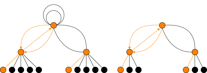
It remains to discuss the action of complex conjugation on the set of directed edges emanating from the surface vertex , which corresponds to “the” elliptic curve with -invariant . By [Cl22a, Thm. 5.3], for any real elliptic curve and any odd prime , there are exactly order -subgroups of stabilized by complex conjugation. When there are two surface loops corresponding to and where are the two -ideals of norm . These two edges are interchanged by complex conjugation (independently of the chosen -structure on ).
So the two real edges must be downward edges. For each real level one vertex , there is a pair of edges from to ; evidently
complex conjugation stabilizes the pair, so if one is real, then both are real. It follows that for exactly one of the two level real
vertices both edges from the surface to that vertex are real, whreas for the other level real vertex neither edge is real. Which is
which depends upon the chosen -structure on : indeed, indeed, for each level real vertex , the unique upward
edge can be defined over and hence over ; this provides an -model for on which the dual
isogeny is real.
If our path starts at and ends up at level then it is clear that the field of moduli is if the path includes a
surface edge and otherwise. The harder case is if our path starts at with and ascends to the surface.
In this case when we ascend to the surface we get the real model for given by the lattice , and in this real model it is the two edges from to that are real. The significance of this for our counting problem is that if we start below
the surface and ascend to the surface there is a unique way to extend the path so that the corresponding isogeny is fixed under
complex conjugation: we take the unique edge from to that is not the inverse of the ascending edge from to .
Thus one sees that in this case we are able to define an action of on , but to do so we had to make a choice that was appropriate for our applications.
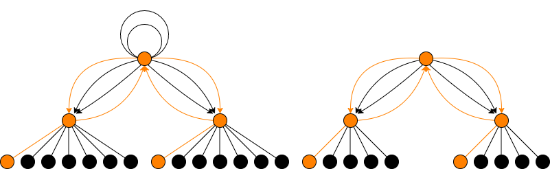
Suppose and . As above, we have and for all . And again, each real vertex in level has an odd number, , of descendant vertices, so has a unique real descendant. If there is a pair of surface loops that are interchanged by complex conjugation; if there are no surface edges. So by [Cl22a, Thm. 5.3] in either -model of “the” elliptic curve with -invariant corresponding to the surface vertex there are precisely order -subgroups stable under complex conjugation. But this time things work out more nicely: there are three edges from to each of the two real level vertices, which as a set are stable under complex conjugation. Since is odd, at least one edge in each set must be fixed by , hence exactly one because there are two such edges altogether.
Suppose and . Now we have , and for all . This means that every vertex of level is real. For each , the real vertices of level can be partitioned into pairs in which each pair has a common neighbor in level , and in each pair, exactly one of the two vertices has two real descendants and the other vertex has no real descendants. This follows from the same argument as in the proof of [Cl22a, Lemma 5.7c)].
Suppose and . We have and for all . For all ,
the vertex corresponding to -invariant is real; the other real vertex in level therefore
must be the other descendant vertex from .
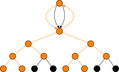
Let us now discuss the action of complex conjugation on edges. Let be “the” elliptic curve of -invariant .
In either -model of , the surface loop corresponds to the isogeny with kernel , where is the unique prime ideal
of lying over , which is stable under complex conjugation.
If we choose the -model of with real lattice , then all three order subgroups are stable under complex conjugation: they can be seen quite clearly as , and
. So it may seem that we have defined an action of
complex conjugation on .
However this graph cannot be used for our study of isogenies! To see why, consider either of the two paths that starts at the
vertex in level , ascends to level , takes the surface loop, and then descends back down to level . These correspond
to two cyclic -iosgenies with source elliptic curve of discriminant . However, contrary to what the graph suggests, neither
of these two isogenies is defined over . Our graph is letting us down because the
surface loop, which can be realized on uniformizing lattices as is an isogeny
of real elliptic curves, but the source and target have different -structures. Recall that every elliptic curve
with has precisely two nonisomorphic -models [SiII, Prop. V.2.2]. When ,
these two models are just quadratic twists of each other, but this is not the case when . When
(i.e., ), for our purposes the most useful way to distinguish between the two models is to observe that in
the model all three order subgroups are real, whereas in the model there is
exaxctly one real order subgroup, generated by . This means that in our length paths considered
above, once we take the surface loop, we arrive at an elliptic curve over for which the two order subgroups that correspond
to the downward edges from to are now interchanged by complex conjugation.
We remedy this by passing from to the double cover by unwrapping the surface loop, to get a graph that now at each level , consists of two copies of the vertex set of
at level . We decree that complex conjugation acts on the second copy of the vertex set the same way it does on the first copy.
The surface edge between the two copies of is real, but in the second copy the two downward edges from to
are now complex. Complex conjugation acts on all other edges in the second copy the same as it does in the first copy (away from the surface the action of complex conjugation on cyclic subgroups is independent of the choice of -model).
Remark 4.2.
-
a)
In Figure 5, we did not draw the upward edge with initial vertex the level vertex in the right hand copy of . As far as the group action of on is concerned, it is clear that this edge must be -fixed. However the -fixedness of this edge has no elliptic curve interpretation – no nonbacktracking path starting in the lefthand copy of in contains this edge. Drawing this edge as -fixed seems to invite confusion, so we have not done so.
-
b)
It’s interesting to compare to the graph of [Cl22a, Lemma 5.7]. These graphs are not isomorphic, but their enumerations of real and complex paths are the same.
-
c)
It is also interesting (and perhaps confusing, at first) to compare the change of real structures induced by the horizontal edge in to the end of the proof of Theorem 4.1, in which the source and target curves of a horizontal edge are rationally isomorphic. The difference is that in the setting of Theorem 4.1 the ground field contains . As for the horizontal edge, it corresponds to the ideal , which is real and principal…but not “real-principal”: i.e., it is not generated by a real element and thus its kernel is not the kernel of an -rationally defined endomorphism.
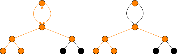
Suppose and . We have for all , so the unique real
vertex in level is , corresponding to the elliptic curve .
There is a sort of “more benign” analogue of the phenomenon encountered in the previous case: the surface loop in this
graph corresponds to the -isogeny . The source and target elliptic curves
are isomorphic over but have different -structures. Indeed, by [BCS17, Lemma 3.2], if and
are real lattices in , then they determine the same -isomorphism class of elliptic curves if and only if they are real homothetic: there is such that . The two lattices
and are not real homothetic: one can see this directly or use [BCS17, Lemma 3.6a)].
So we defined an action of complex conjugation on the three downward edges with initial vertex the surface vertex : one
is real and two are complex. After we take the surface loop we are now considering the action of complex conjugation on a
nonisomorphic real elliptic curve. Because of this, the principled response is to again pass from
to the double cover by unwrapping the surface loop to get a
graph that at each level consists of two copies of the vertex set of at level , and we define the action of
complex conjugation in the same way as above.
While in the previous case the change of -structure changed the number of order subgroups fixed by complex conjugation, in this case , so [Cl22a, Thm. 5.1] applies to show that in any -model exactly one of the three “downward” order subgroups is real. So while in the previous case we needed to pass to the double cover in order to ensure the correctness of our enumeration of real and complex paths, in this case the enumeration of real and complex paths is the same whether we pass from to or not.
5. CM Points on
Let be a prime number, and let be an imaginary quadratic discriminant with . In this section we will compute the fiber of over . For there is no ramification,
so we determine which residue fields occur and with what multiplicity. For , a closed point on in the fiber over has ramification, of index or in the respective cases of and , exactly when a path in its closed point equivalence class includes a descending edge from level to level , i.e. exactly when the path is not completely horizontal. The residue field of a closed point on a finite-type -scheme is a number field that is well-determined up to isomorphism; it is not well-defined as a subfield of . Thus when we write that
the residue field is for some , we mean that it is isomorphic to this field.
Without loss of generality we may take our source elliptic curve to have -invariant . Our task is then to:
(i) Enumerate all nonbacktracking length paths in .
(ii) Sort them into closed point equivalence classes , and record the field of moduli for each equivalence
class (we record any number field isomorphic to as ).
(iii) Record how many closed point equivalence classes give rise to each field of moduli.
In §3.4 we have addressed the added subtlety in the notion of backtracking when , and in §4.2 we have provided a meaningful description of the action of complex conjugation on paths in . This provides the means to carry out our path-type analysis steps (i) through (iii), just as done in [Cl22a, §7] for . What we find is that the resulting enumeration of path types and corresponding residue fields for is exactly as in [Cl22a, §7] for any given and splitting behavior of in , and so we refer the reader to the enumeration provided therein.
A check on the accuracy of our calculations is as follows: let be the multiplicative function such that
for any prime power we have . For all , we have (e.g. [CGPS22, Lemma 4.1a)])
Letting and denote, respectively, the residual degree and ramification index of the closed point with respect to the map , we must have
where the sum extends over closed point equivalence classes of points in the fiber over .
6. The Projective Torsion Field
Let be a field of characteristic , let be an elliptic curve, and let . The projective -torsion field is the kernel of the modulo projective Galois representation, i.e., the composite homomorphism
where denotes the projectivization of the -dimensional -module . After choosing a -basis
for , we may view as a homomorphism from to . Thus is a finite degree
Galois extension. The projective -torsion field of is also characterized as the minimal algebraic extension of over which all cyclic -isogenies with source elliptic
curve are defined.
The following result is a small refinement of [BC20a, Prop. 4.5].
Proposition 6.1.
Let be an imaginary quadratic discriminant, let , and let be a -CM elliptic curve.
-
a)
The following are equivalent:
-
(i)
We have .
-
(ii)
There is a -rational cyclic -isogeny , where is an -CM elliptic curve.
-
(i)
-
b)
For every -CM elliptic curve , there is an elliptic curve with and such that satisfies the equivalent conditions of part a). Moreover, an elliptic curve with satisfies the equivalent conditions of part a) if and only if is a quadratic twist of .
Proof.
As usual, it is no loss of generality to assume that .
a) The implication (ii) (i) follows from [BC20a, Prop. 4.5] and its proof. As for (i) (ii), we may take to
be the dual of the isogeny , which because of (i) must be -rational on .
b) The isogeny is defined over , hence also over . Since , the -rational
model of an elliptic curve with -invariant is unique up to quadratic twist. If is a field of characteristic different
from , is an -rational isogeny with kernel , and , then
remains -rational on the quadratic twist and we have . This shows that the elliptic curve
of part b) exists and is unique up to quadratic twist; finally, quadratic twists do not change rationality of isogenies hence
do not change projective torsion fields.
∎
For an imaginary quadratic discriminant , let be the imaginary quadratic order of discriminant and let
Theorem 6.2.
Let be an imaginary quadratic discriminant, and let .
-
a)
Let be a -CM closed point. Then .
-
b)
Let be a field of characteristic , and let be a -CM elliptic curve. Then and .
Proof.
Again we may assume without loss of generality that .
a) By Proposition 6.1, there is a -CM elliptic curve on which the projective modulo Galois representation
is trivial. This elliptic curve induces a -CM closed point such that can be embedded into .
Moreover, in the notation of [Cl22a, §1.1], the subgroup of used to define the modular curve is the subgroup of scalar matrices, which is normal, hence is a Galois covering of curves over . It follows that all residue fields of closed points of lying over the closed point of are isomorphic. It
follows that is isomorphic to a subfield of . By [DR73, Prop. VI.3.2] there is an elliptic curve
inducing with trivial projective modulo Galois representation. As in the proof of Proposition 6.1
we have a -rational isogeny with , so contains . Since , we have
either or . However, if , then since , we get a real elliiptic curve with
real projective -torsion field, contradicting [Cl22a, Cor. 5.4].
b) From part a) we know that . Consider the base
extension of to . It follows from part a) that there is a character
such that the twist of by has trivial projective mod Galois representation. There is then a cyclic field extension of degree dividing such that
which means that there is a quadratic twist of for which the projective mod Galois representation is trivial. But quadratic twists do not affect the projective modulo Galois representation, so the projective Galois representation on is trivial, and . ∎
When , the projective -torsion field of an elliptic curve is just its -torsion field . Because of this the analogue of Theorem 6.2 had already been known, but for future reference we record the result anyway.
Proposition 6.3.
Let be an imaginary quadratic discriminant, let be a field of characteristic , and let be a -CM elliptic curve. Let be a -CM point. Then:
-
a)
If is odd, then .
-
b)
If is even, then .
-
c)
If , then .
-
d)
If , then .
Proof.
Again, because is a Galois covering, all the residue fields of on lying over
the closed point of are isomorphic.
a),b) Suppose . The results follow from [BCS17, Thm. 4.2] together with the observation that there is a point of order on such that has -CM. (They can also be obtained from an analysis of -isogeny graphs.)
c) The -CM elliptic curve has .
d) For all , the curve
is a -CM elliptic curve with . Each of these fields contains , so . Moreover , so . ∎
7. Primitive Residue Fields of CM points on
Let be an imaginary quadratic discriminant, let be a prime and let be integers. In this section we extend the work of [Cl22a, §7], determining all primitive residue fields and degrees of -CM points on , to the cases in which .
It is no loss of generality to assume that the -invariant of our -CM elliptic curve is , and we shall do so throughout
this section.
For a modular curve, we call the residue field of a closed -CM point a primitive residue field of -CM points on if there is no other -CM point together with an embedding of the residue field into as a proper subfield. We call the degree a primitive degree of -CM points on if there is no -CM point such that properly divides .
Throughout this section, when working with a -CM point we put
7.1.
In the case of , i.e., of , our results of §5 imply immediately that the case analysis is exactly as in [Cl22a, §8.1]. We recall the answer here for completeness:
Case 1.1: Suppose .
Case 1.1a: Suppose . The primitive residue field is (which equals
when ).
Case 1.1b: Suppose . The primitive residue field is .
Case 1.2: Suppose and . The primitive residue fields
are and .
Case 1.3: Suppose and . The primitive residue field is .
Case 1.4: Suppose , and . The primitive residue
field is .
Case 1.5: Suppose , and .
Case 1.5a: Suppose . In this case there is a -rational cyclic -isogeny, so the only primitive
residue field is .
Case 1.5b: Suppose . Then the primitive residue fields are and .
Case 1.6: Suppose , , and .
Case 1.6a: Suppose . As in Case 1.5a, there is a -rational cyclic -isogeny, so the only primitive
residue field is .
Case 1.6b: Suppose . In this case the primitive residue field is .
Case 1.7: Suppose , , .
Case 1.7a: Suppose . As in Case 1.5a, there is a -rational cyclic -isogeny, so the only primitive
residue field is .
Case 1.7b: Suppose . In this case the primitive residue field is .
Case 1.8: Suppose , , , and .
Case 1.8a: Suppose . The primitive residue fields are and .
Case 1.8b: Suppose and . The primitive residue field is .
Case 1.8c: Suppose and . The primitive residue fields are and .
Case 1.9: Suppose , , , and .
Case 1.9a: Suppose . The primitive residue fields are and .
Case 1.9b: Suppose and . The primitive residue field is .
Case 1.9c: Suppose and . The primitive residue fields are and .
Case 1.10: Suppose , , , , and .
Case 1.10a: Suppose . The primitive residue field is .
Case 1.10b: Suppose . The primitive residue fields are and .
Case 1.11: Suppose , , , , and .
Case 1.11a: Suppose . The primitive residue field is .
Case 1.11b: Suppose . The primitive residue field is .
7.2. A field of moduli result
Now suppose that are integers, and let be a closed -CM point. Then we have morphisms
Theorem 7.1.
Let be a prime number, let be positive integers and let be a closed -CM point.
-
a)
We have
-
b)
We have if any of the following conditions holds:
-
(i)
.
-
(ii)
.
-
(iii)
.
-
(i)
Proof.
Since is an extension of both and , clearly
If , then conversely : indeed, in this case, the projective torsion field
is independent of the model. So we may suppose .
Step 2: We will show that
| (4) |
Since , the point corresponds to a path of length with initial vertex at the surface; if the terminal vertex has level , then , so if we put
then
We may factor an isogeny inducing as
where is horizontal and is descending of length . By the results of §6, there is an
elliptic curve with -invariant on which the modulo Galois representation
is given by scalar matrices. The point is induced by a cyclic -isogeny of -elliptic curves ;
since , this isogeny factors as , where is horizontal of degree and is descending of degree . We claim that every isogeny of this form is defined over . Indeed, as in the proof of Theorem 4.1 we have that is defined over
and moreover . It follows that the modulo -Galois representation on is given by
scalar matrices, so is also defined over and thus is as well.
Step 3: By Theorem 6.2 and Proposition 6.3 we have that if either or is odd. Thus in either of these cases we have
| (5) |
Step 4: Finally, if then is the identity map, so holds trivially. ∎
Corollary 7.2.
Let , and let be a -CM point. Let be an isogeny of complex elliptic curves inducing .
-
a)
If is purely descending, then .
-
b)
Otherwise, .
Proof.
Since , there are precisely two possibilities for : it either consists
of descending edges, or it has one horizontal edge followed by descending edges.
In the former case, we have
. Moreover, on the model of that makes -rational, we evidently have a
descending -rational -isogeny. As for any -CM elliptic curve defined over , we have a horizontal
-rational -isogeny. Thus the -action on the three order subgroup schemes of fixes
two of the subgroups, so it must also fix the third. We conclude that in this case.
Now suppose that consists of a horizontal edge followed by descending edges. Now , which is real number field, so if then we would have , a real number field. But
as we saw in §4.2, the horizontal -isogeny on a real ellliptic curve with -invariant interchanges the two -structures on this elliptic curve, and on precisely one of the two -structures do we have an -rational descending -isogeny.
If then we would have -rational descending -isogenies defined on both the source and target of ,
which is not possible. Therefore in this case , so by Theorem 7.1 we have .
∎
7.3.
Using Theorem 7.1, Corollary 7.2 and the work of §5 and §6, it is easy to compute all primitive residue fields of -CM
points . Indeed:
Suppose . Then for any -CM point , equation (5) applies. So if is the minimal level such that there is a nonbacktracking path in
starting in level (where ), the unique primitive residue field is . So:
Case 2.1: If , the primitive residue field is .
Case 2.2: If , the primitive residue field is .
Case 2.3: If , the primitive residue field is .
Suppose and is odd. Again equation (5) applies and the unique
primitive residue field is . So:
Case 3.1: If , the primitive residue field is .
Case 3.2: If and , the primitive residue field is .
Case 3.3: If and , the primitive residue field is .
Suppose and is even. For a -CM point Theorem 7.1 and Corollary 7.2 tell us that if , if or if an isogeny inducing is purely descending then
and otherwise we have .
Our casework for -CM points on is then as follows:
Case 4.0: . The primitive residue field is .
Case 4.1: , and . The primitive residue fields are and .
Case 4.2: , and . The primitive residue field is .
Case 4.3: , and . The primitive residue fields are and .
Case 4.4: , and . The primitive residue field is .
Case 4.5: , and . The primitive residue fields
are and .
Case 4.6: , and . The primitive residue fields are
and .
Case 4.7: , and . The primitive residue
fields are and .
Case 4.8: , and . The primitive residue field is .
Case 4.9: , and . The primitive residue fields are
and .
Case 4.10: , and . The primitive residue fields are
and .
Case 4.11: , and . The primitive residue field is .
Case 4.12: , and . The primitive residue fields are
and .
Case 4.13: , and . The primitive residue field is .
Case 4.14: , and . The primitive residue field is .
8. CM points on
Throughout this section is an imaginary quadratic discriminant with , and are positive integers. We now discuss how to use our work developed thus far to determine the -CM locus on . In §8.1 we recall how the compiling across prime powers process works for , and in §8.2 we provide a result for compiling across prime powers for . In the remainder of this section, we give an explicit description of all primitive residue fields and primitive degrees in this case.
8.1. Compiling Across Prime Powers with
For this section, we suppose with . With this assumption, [Cl22a, Prop. 3.5] applies and our compiling across prime powers process works much the same as in [Cl22a, §9.1]. We elaborate here for completeness of our discussion.
For a prime and integers , the fiber of over the closed point is a finite étale -scheme, i.e. is isomorphic to a product of finite degree field extensions of . Our work up to now shows that the residue field of any CM point on is either a ring class field or a rational ring class field, and so there are non-negative integers such that , where
| (6) |
When , the explicit values of the ’s and ’s can be determined from our results in §5. When or is odd, by Theorem 6.2 we have for all .
We now explain how the previous results allow us to compute the fiber of over for any positive integers , where and . For , let be the fiber of over . By [Cl22a, Prop 3.5] we have
| (7) |
It follows that is isomorphic to a direct sum of terms of the form
where for we have that is isomorphic to either for some or to for some .
Let be the number of indices such that is contained in , i.e. such that . Because , Proposition 2.2 gives:f
(Note that can only occur if , due to our assumption.) We therefore reach the following extension of [Cl22a, Theorem 9.1]:
Theorem 8.1.
Let be an imaginary quadratic discriminant with . Let . Let be a -CM closed point on .
-
a)
The residue field is isomorphic to either or for some .
-
b)
Let , be the prime power decompositions of and . For , let be the natural map and put . The following are equivalent:
-
(i)
The field is formally real.
-
(ii)
The field does not contain .
-
(iii)
For all , the field is formally real.
-
iv)
For all , the field does not contain .
-
(i)
8.2. Compiling Across Prime Powers with
Throughout this section, we assume that .
Proposition 8.2.
Suppose that is a cyclic -isogeny, with having prime-power factorization . For each , let be the -primary part of . Let such that is isomorphic to either or to . Then
Proof.
Let , and for each let be the Sylow- subgroup of , that is . Let denote the conductor of , and for let denote the conductor of . Let
and let
Then factors as , where . Using the fact that isogenies of degree prime to cannot change the -part of the conductor, we see that has conductor divisible by . Thus we have
It remains to show the containment . If , then this follows from Theorem 4.1 and [Cl22a, Prop. 3.5], so we suppose . If , then is (up to isomorphism on the target) an endomorphism of , hence defined over . If then , so our previous work applies via consideration of the dual isogeny as . ∎
Proposition 8.2 provides bounds on the field of moduli of an isogeny. We now use this result to determine the exact field of moduli in the case where our source elliptic curve has -CM or -CM, which we state from the perspective of determining the residue field of the corresponding CM point on
Theorem 8.3.
Let with prime-power factorization , and suppose is a -CM point with . Let be the natural map, and let . Let be any path in the closed point equivalence class corresponding to in , and let be the number of descending edges in .
-
a)
If there is some such that splits in and the path contains a surface edge, then
-
b)
In every other case, we have
Proof.
Let be a cyclic -isogeny inducing the point . For each , let
be the -primary part of : that is, the kernel of is the -Sylow subgroup of
the kernel of .
Case 1: Suppose that is also a -CM elliptic curve. By [Cl22a, §3.4], the isogeny is isomorphic over
to for a nonzero ideal of , and we have if is real ideal (i.e., and is is not a real ideal. If we factor into prime powers and
lies over , then we have (up to an isomorphism on the target) that .
Notice that the path in corresponding to lies
entirely on the surface. If some splits in , then is not a real ideal, so . If no splits in , then each is real, so is real and .
Case 2: Otherwise is a -CM elliptic curve for some . Since ,
we may compute the field of moduli of the dual isogeny . Since , the rationality of
a subgroup of is independent of the model, so we have , and the result
now follows from [Cl22a, Thm. 5.1].
∎
Corollary 8.4.
Let be an isogeny of -CM elliptic curves defined over . Let (resp. ) be the conductor of (resp. of ). Then the field of moduli of contains a subfield isomorphic to .
Proof.
When , then Corollary 8.4 holds just because . However:
Corollary 8.5.
Let , let be coprime positive integers not lying in the set of Proposition 2.1: that is, if then and if then . Let be an isogeny of -CM elliptic curves defined over such that has conductor and has conductor . Then cannot be defined over .
Next we obtain a version of Theorem 8.3 in the case, finding in particular that the residue field of a CM point on is isomorphic to either a rational ring class field or a ring class field in all cases.
Theorem 8.6.
Let with , and write
Let
and
be the canonical maps. Let , let be a -CM closed point of and let . Let be the number of descending edges in , and put
-
a)
Suppose or ( and ). Then
-
b)
Suppose and ; we put .
-
(i)
If and is not purely descending, then
-
(ii)
Otherwise, we have
-
(i)
Proof.
a) Our hypotheses on imply (cf. §6) that
In particular, this implies that . Applying Proposition 8.3 we get
Using this and Proposition 2.1a), we get:
Conversely, using Proposition 6.1, let be an elliptic curve with -invariant
and with modulo -Galois representation given by scalar matrices.
For , let be a cyclic
-isogeny of -elliptic curves containing descending edges. It follows from the proof of Theorem 7.1,
that the kernel of is a -rational subgroup scheme, hence
so is , which is the kernel of . Thus we have found a -rational model of .
b) (i) By Corollary 7.2, we have . The rest of the argument is the same as that
of part a).
(ii) First, suppose that is purely descending and let be an isogeny defined over that induces the point . Then the initial
edge of is downward, so as in the proof of Corollary 7.2 every order subgroup of is -rational. This provides , and the stated isomorphism then follows from Proposition 8.3.
Lastly, suppose that and that the -isogeny inducing is horizontal. This final case can be reduced to the previous one via automorphisms of the modular curve . Indeed, observe that the map is a Galois cover. The level -structure associated to may viewed as an elliptic curve equipped with an ordered triple , where is a cyclic subgroup of of order and and are distinct cyclic subgroups of of order . The map can then be viewed as . The action fixes and , and on the pair the action is the natural and simply transitive one on pairs of order subgroups of . Therefore if is induced by a tuple with a horizontal -isogeny, then is necessarily descending and we have where is induced by . By the previous case, we have that
is the field of moduli of the isogeny . Again, the stated isomorphism follows via Proposition 8.3. ∎
Theorems 8.3 and 8.6 are the key ingredients for the determination of primitive residue fields and primitive degrees of -CM points on , which we will provide in the next section. However, there remains the problem of computing the set of all -CM points on with a given rational ring class field or ring class field as residue field. The following results solve this problem.
Theorem 8.7.
Let have prime power factorization . For , let be a -CM point, and let denote the natural map. Let be the set of closed points such that for all . Put
If , then . If , then consists of points, each with residue field the same ring class field.
Proof.
Step 1: Suppose that . Let be the fiber of over , and for let be the fiber of over . Then by [Cl22a, Prop. 3.5] we have that is the fiber
product of over . By our hypothesis, we have either or . If ,
the result follows from this and [Cl22a, Prop. 2.10], as is recorded in [Cl22a, §9.1]. If
and , the result follows from this and Proposition 2.2.
For the remainder of the argument we suppose that . Let , let be
an isogeny inducing the point , and put . The endomorphism ring of has
discriminant for some .
Step 2: We suppose that . For each , let and be the
isogeny . Then factors as , wehre is a cyclic -isogeny. Let be the conductor of the endomorphism ring of , so , since
the conductor of is and is prime to .
For , the path in corresponding to therefore terminates at the unique
surface vertex, hence it consists of ascending edges, which are uniquely determined by , followed by
horizontal edges. If does not split in the path corresponding to is
therefore uniquely determined, whereas if splits in there are two such paths which are complex conjugates of each other and therefore determine the same closed point equivalence class. Let be the -CM point induced by
, and let be the set of closed points such that for all .
Thus passage to the dual isogeny gives a residue-field preserving bijection from to . Let .
Because the path corresponding to begins at the surface and the path corrsesponding to ends at the surface, we have that contains if and only if splits in in if and only if contains .
Applying Step 1, we get that if then , while if then
Step 3: We suppose that . In this case every element of is induced by an isogeny for a nonzero -ideal such that is cyclic, and . Moreover the field of moduli of is if and otherwise [Cl22a, §3.4]. For distinct and , the isogenies and induce the same closed point on if and only if , so closed point equivalence classes in this case correspond to orbits under . For a prime power , there is an ideal of norm such that is cyclic if and only if ( ramifies in and ) or splits in . In the ramified case there is a unique ideal of norm , while in the split case the two ideals of norm are and where and are the two primes of lying over . If is the number of such that splits in , then if then the unique prime number that ramifies in so . If , then the number of ideals of norm such that is cyclic is , and the number of -orbits of such ideals is . ∎
Corollary 8.8.
Let be in with prime-power factorizations and with . Let denote the natural map, and let denote the natural map for . Let be -CM points for each index , and let be the set of closed points such that for all . For each , let denote the number of descending edges occurring in a path in corresponding to . Put
and put
We then have that consists of
points with isomorphic residue fields.
Proof.
Given a point , Theorem 8.6 determines the residue field of any point in terms of and , so we know that each point in has the same residue field up to isomorphism. If then the map is unramified. If (resp. ), then the map has ramification index if and only if the path in corresponding to is purely horizontal for each . Therefore, because (see the discussion in §1.4 for more details), the point necessarily has ramification index (resp. ) exactly with respect to in this situation, and otherwise has ramification index . In any event, letting be a point with for all , we must have that the number of points lying above is
The case, by Theorem 8.6, is exactly the case in which is isomorphic to a rational ring class field while is a ring class field. In the case, we then have
while the only change in this quantity in the case is an additional factor of . This combined with the result of the previous theorem gives the result as stated. ∎
8.3. Primitive Residue Fields and Primitive Degrees I
In this section and the next, we extend the results of [Cl22a, §9.2-9.3] to handle . Given our extensions of the results on primitive residue fields of -CM points on for prime and on compiling across prime powers this proceeds nearly exactly as therein.
In this section, as in [Cl22a, §9.2], we suppose that either or that ( and is even). This assumption implies that there is a closed -CM point on with residue field isomorphic to , and therefore there is a unique such that is a primitive residue field of -CM points on . For each , take to be the least integer such that is isomorphic to the residue field of a -CM point on . We then have
There is at most one other primitive residue field of a -CM point on , and there is one other exactly when there are two primitive residue fields for -CM points on for some . In this case, letting , for , be the least natural number such that there is a -CM point on with residue field isomorphic to either or to , we have that the other primitive residue field is , where
If there is a unique primitive residue field of -CM points on , then of course there is a unique primitive degree of such points. Supposing we are in the case of two primitive residue fields and , we put
We will have a unique primitive degree if and only if one of and divides the other, and we will soon see that we always have , so the question is whether . This divisibility certainly holds if the analogous divisibility holds at every prime power, but as seen in [Cl22a] this is not a necessary condition. The following theorem determines exactly the situation, generalizing [Cl22a, Thm. 9.2]. The proof is only mildly more complicated than the proof of this prior result, owing to handling the case.
Theorem 8.9.
Let be an imaginary quadratic discriminant, and let . We suppose that either or ( and is even). For , let be the unique natural number such that occurs up to isomorphism as a primitive residue field of a closed -CM point on . Let be equal to if there is a unique primitive residue field of -CM points on and otherwise let it be such that the unique non-real primitive residue field of a closed -CM point on is . Put and . Let be the number of such that there is a non-real primitive residue field of a closed -CM point on .
-
a)
If , the unique primitive residue field of a -CM point on is , so the unique primitive degree of a -CM point on is .
-
b)
If and there is some such that there are two primitive residue fields of closed -CM points on and we are not in Case 1.5b) with respect to and , then:
-
(i)
There are two primitive residue fields of -CM points on : and .
-
(ii)
The unique primitive degree of -CM points on is .
-
(i)
-
c)
If and for all such that there are two primitive residue fields of closed -CM points on we are in Case 1.5b), then there are two primitive degrees of -CM points on : and .
Proof.
The case is immediate from the above discussion. Henceforth we suppose . We then have (up to isomorphism) two primitive residue fields of -CM closed points on : and , and as above we put
For each , let be a primitive residue field of a closed point of a -CM elliptic curve on ; if there is any non-real such field, take to be nonreal. Note that for each such that there are two primitive residue fields and we have ]. By Propositions 2.1 and 2.2, there is such that
It follows that . Thus there is a unique primitive degree exactly when , as claimed in the above discussion.
Because , we have . In particular, we have
for every odd prime .
Case 1: Suppose . By Proposition 2.1 we have
It follows that if and only if there is some such that there are two primitive residue fields of -CM closed points on for which we have
which holds if and only if
This holds in every case in which there are two primitive residue fields except Case 1.5b).
Case 2: Suppose . Let be the number of indices such that , and let be the number of indices such that . We have . Proposition 2.1 then gives:
and
We see then that if and only if
We find that if and only if or there is some such that for which we are
not in Case 1.5b) with respect to and . Comparing with the statement of the result, we must show:
in every case in which there is some for which and we are not in Case 1.5b) for
and . So:
If , then , so there are two primitive degrees if and only if we are in Case 1.5b)
for all for which , as claimed.
If then Case 1.5b) cannot occur for any and thus , as claimed.
∎
8.4. Primitive Residue Fields and Primitive Degrees II
In this section we treat the case in which either , or ( and is odd). Thanks to the work of §7, this case follows exactly as in [Cl22a, §9.3]. In particular, our assumptions imply that there is a unique primitive residue field, which is a ring class field .
Let and . For an index , if the only primitive residue field of a -CM point on is then put . Otherwise, the primitive residue fields of -CM points on are of the form and , and we put . We then have
References
- [BC20a] A. Bourdon and P.L. Clark, Torsion points and Galois representations on CM elliptic curves, Pacific J. Math. 305 (2020), 43–88.
- [BC20b] A. Bourdon and P.L. Clark, Torsion points and rational isogenies on CM elliptic curves. J. Lond. Math. Soc. (2) 102 (2020), 580–622.
- [BCS17] A. Bourdon, P.L. Clark and J. Stankewicz, Torsion points on CM elliptic curves over real number fields. Trans. Amer. Math. Soc. 369 (2017), 8457-–8496.
- [CGPS22] P.L. Clark, T. Genao, P. Pollack and F. Saia, The least degree of a CM point on a modular curve. J. Lond. Math. Soc. (2) 105 (2022), 825–883. http://alpha.math.uga.edu/~pete/least_CM_degree-1226.pdf
- [Cl22a] P.L. Clark, CM elliptic curves: volcanoes, reality and applications, Part I.
- [Cx89] D. Cox, Primes of the form . Fermat, class field theory and complex multiplication. John Wiley Sons, New York, 1989.
- [DR73] P. Deligne and M. Rapoport, Les schémas de modules de courbes elliptiques. Modular functions of one variable, II (Proc. Internat. Summer School, Univ. Antwerp, Antwerp, 1972), pp. 143–316. Lecture Notes in Math., Vol. 349, Springer, Berlin, 1973.
- [DS05] F. Diamond and J. Shurman, A first course in modular forms. Graduate texts in mathematics, 228. Springer, New York, 2005.
- [LLS15] Y. Lamzouri, X. Li and K. Soundararajan, Conditional bounds for the least quadratic non-residue and related problems. Math. Comp. 84 (2015), 2391–2412.
- [SiI] J.H. Silverman, The arithmetic of elliptic curves. Second edition. Graduate Texts in Mathematics, 106. Springer, Dordrecht, 2009.
- [SiII] J.H. Silverman, Advanced Topics in the Arithmetic of Elliptic Curves, Graduate Texts in Mathematics 151, Springer-Verlag, 1994.
- [Su12] A.V. Sutherland, Isogeny volcanoes. https://arxiv.org/abs/1208.5370