Coarse reduced model selection for nonlinear state estimation

Complex physical systems are often modelled by a parametric partial differential equation (PDE). We consider the general problem of the form

where $A(y):\mathcal{H}\to\mathcal{H}^{\prime}$ is an elliptic second order operator, $\mathcal{H}$ is an appropriate Hilbert space. The problem is defined on a physical domain $D\subset\mathbb{R}^{2,3}$, and the parameter $y$ is within a parameter domain $\mathcal{Y}$, typically a subset of $\mathbb{R}^{d}$ where $d$ might be large. Each parameter $y\in\mathcal{Y}$ is assumed to result in a unique solution $u(x,y)$ but we mostly suppress the spatial dependence $x\in D$ and write $u(y)$. We denote all $\mathcal{H}$-norms by $\|\cdot\|:=\|\cdot\|_{\mathcal{H}}$ and inner-products $\langle\cdot,\cdot\rangle:=\langle\cdot,\cdot\rangle_{\mathcal{H}}$, and use an explicit subscript if they are from a different space.

In practical modelling applications it is often computationally expensive to produce a high precision numerical solution to the PDE problem (1). To our advantage however, the mapping $u:y\to\mathcal{H}$ is typically smooth and compact, hence the set of solutions over all parameter values will be a smooth manifold, possibly of finite intrinsic dimension. We define the solution manifold as follows, assuming from here that it is compact,

The methods proposed in this paper extend on reduced basis approximations. A reduced basis is a linear subspace $V\subset\mathcal{H}$ of moderate dimension $n:=\dim(V)\leq\dim(\mathcal{M})\leq\dim(\mathcal{H})$. We use the worst-case error as a benchmark, defined as

where $P_{V}$ is the orthogonal projection operator on to $V$. There are a variety of methods to construct a reduced basis with desirable worst-case error performance, and here we concentrate on greedy methods that select points in $\mathcal{M}$ which become the basis for $V$. We discuss these methods further in §1.1.

A reduced basis can be used to accelerate the forward problem. One can numerically solve the PDE problem for a given parameter $y$ by using $V$ directly in the Galerkin method, making the numerical problem vastly smaller while retaining a high level of accuracy. A thorough treatment of the development of reduced basis approximations is given in [5].

In this paper we are concerned with inverse problems. In this setting it is assumed that there is some unknown true state $u$ (which could correspond to the state of some physical system), and we do not know the parameter vector $y$ that gives this solution. Instead, we make do with a handful of $m$ linear measurements $\ell_{i}(u)$. These measurements are used to make some kind of accurate reconstruction of $u$ (state estimation) or a guess of the true parameter $y$ (parameter estimation).

The Parametrized Background Data Weak (PBDW) approach introduced in [6] gives a straightforward procedure for finding an estimator $u^{*}$ of the true state $u$, using only the linear measurement information and a reduced basis $V$. One limitation however is that the estimator error $\|u^{*}-u\|$ is bounded from below by the Kolmogorov $n$-width given by

where the infimum is taken over all $n$ dimensional linear spaces in $\mathcal{H}$. The $n$-width is known to converge slowly for many parametric PDE problems.

We will review methods for constructing a family of local linear reduced models and a nonlinear estimator $u^{*}$ using a surrogate distance model selection procedure. We propose the use of coarser finite element meshes to perform this selection. This coarse selection strategy is motivated by the observation in [3] that the model selection is by far the most computationally costly component in the nonlinear estimation routine. Finally in §4 we examine numerical examples of surrogate distances over different mesh widths, and see that they make insubstantial impacts to the nonlinear estimator.

A fundamental drawback of linear reduced models is the slow decay of the Kolmogorov $n$-width for a wide variety of PDE problems. To circumvent this limitation, a framework for non-linear reduced models and their use for state estimation was presented in [3]. The proposal involves determining a partition of the manifold

and producing a family of affine reduced space approximations $V_{k}$ to each portion $\mathcal{M}_{k}$. Each space has dimension $n_{k}=\dim(V_{k})$, requiring $n_{k}<m$ for well-posedness.

Given any target $\varepsilon>0$ and $\mu\geq 1$ it is possible with large enough $K$ to determine a partition and family of reduced spaces $V_{k}$ that satisfies

in which case we say the family $(V_{k})_{k=1}^{K}$ is $(\mu,\varepsilon)$-admissible. A slightly looser criteria on the partition can also be satisfied: given some $\sigma>0$, we say the family $(V_{k})_{k=1}^{K}$ is $\sigma$-admissible if $\mu_{k}\varepsilon_{k}\leq\sigma$ for all $k=1,\ldots,K$. The existence of both $(\mu,\varepsilon)$ and $\sigma$-admissible families follow from the compactness of $\mathcal{M}$, and a full demonstration can be found in [3].

In practice one may construct a $\sigma$-admissible family in the following way. Say we are given a partition of the parameter space $(\mathcal{Y}_{k})_{k=1}^{K-1}$ with $\cup_{k=1}^{K-1}\mathcal{Y}_{k}=\mathcal{Y}$, and the associated partition of the manifold $(\mathcal{M}_{k})_{k=1}^{K-1}$. We have a reduced space $V_{k}$, produced by a greedy algorithm on each $\mathcal{M}_{k}$. With each $V_{k}$ we have an associated error estimate $\sigma_{\mathrm{est,k}}=\mu_{k}(V,W)\varepsilon_{\mathrm{est},k}(V,\mathcal{M})$. We can pick the the largest $\sigma_{\mathrm{est,k}}$, with index $\tilde{k}$ say, and we split the cell $\mathcal{Y}_{\tilde{k}}$ in half for each parameter coordinate direction $i\in\{1,\ldots,d\}$, resulting in two reduced spaces $V_{\tilde{k},i}^{+}$ and $V_{\tilde{k},i}^{-}$ for each split direction. We take the split direction $i$ to be the one with the smallest maximum error $\max(\sigma_{\tilde{k},i}^{+},\sigma_{\tilde{k},i}^{-})$, and we enrich the family $(V_{k})_{k=1}^{K-1}$ with the two new reduced spaces, making sure to remove $V_{\tilde{k}}$ from the collection. More details of the splitting procedure can be found in [3].

Say the operator $A(y)$ in (1) is uniformly bounded in $y$ with uniformly bounded inverse, that is for some $0<r\leq R<\infty$ we have

Then we can show that for any $v\in\mathcal{H}$ the residual of the PDE,

satisfies the uniform bound $r\|v-u(y)\|\leq\mathcal{R}(v,y)\leq R\|v-u(y)\|$. If we define the following,

then we have arrived at a surrogate distance that satisfies the uniform bounds of (8). Using this surrogate in the selection (9) to define $u^{*}(w)$, we have a nonlinear reconstruction algorithm with the error guarantees of (10).

We now make the further assumption that the operator $A(y)$ and source term $f(y)$ have affine dependence on $y$, that is

The residual can be calculated using representers in $\mathcal{H}$. We define $e_{j}$ as member of $\mathcal{H}$ that satisfies

and now write $e(y):=e_{0}-\sum_{j=1}^{d}y_{j}e_{j}$ to denote the representer of the overall residual problem. The residual is equal to $\mathcal{R}(v,y)=\|e(y)\|$, and determining the surrogate distance is a quadratic minimisation problem

This leads to a constrained least squares problem that can be solved using standard optimisation routines, using the values $\langle e_{i},e_{j}\rangle$ for $0\leq i,j\leq d$.

We present two separate studies of the surrogate as evaluated in finite element spaces. On the unit square $D=[0,1]^{2}$ we consider the PDE

where our parametric diffusivity field is given by $a(x,y)=1+\sum_{j=1}^{16}c_{j}y_{j}\raise 1.29167pt\hbox{\large$\chi$}_{D_{j}}(x)$. Here the $D_{j}$ denote squares of side length $1/4$ that subdivide the unit square in to 16 portions, and $\raise 1.29167pt\hbox{\large$\chi$}_{D_{j}}$ is the indicator function on $D_{j}$. The parameter range is the unit hypercube $\mathcal{Y}=[-1,1]^{16}$, and the coefficients are $c_{j}=0.9j^{-1}$ or $c_{j}=0.99j^{-1}$, meaning that $a(x,y)>0$, but when $c_{j}=0.99j^{-1}$ the $a(x,y)$ can become closer to 0 hence the PDE problem can lose ellipticity.

We perform space discretisation by the Galerkin method using $\mathbb{P}_{1}$ finite elements to produce solutions $u_{h^{\prime}}(y)$, with a fine triangulation on a regular grid of mesh size $h^{\prime}=2^{-7}$. In the tests that follow, we will evaluate $\mathcal{S}_{h}(v,\mathcal{M})$ with coarse meshes of size $h=2^{-s}$ with $s=2,\ldots,6$.

We generate training sets to compute the reduced models, and test sets on which we test the reconstruction algorithms. The training set $\widetilde{\mathcal{M}}^{\mathrm{tr}}$ is taken to be the collection of PDE solutions for $N_{\mathrm{tr}}=1000$ random samples $\widetilde{\mathcal{Y}}^{\mathrm{tr}}=\{y^{\mathrm{tr}}_{j}\}_{j=1,\ldots,N_{\mathrm{tr}}}$ drawn independently and uniformly on $\mathcal{Y}=[-1,1]^{16}$. The test set $\widetilde{\mathcal{M}}^{\mathrm{te}}$ is created from $N_{\mathrm{te}}=100$ independent parameter samples that are distinct from the training set samples.

In our test the measurement space $W$ is given by a collection of $m=8$ measurement functionals $\langle\omega_{i},u\rangle=\ell_{i}(u)=|B_{i}|^{-1}\int u\,\raise 1.29167pt\hbox{\large$\chi$}_{B_{i}}$ that are local averages in a small area $B_{i}$ which are boxes of width $2h=2^{-6}$, each placed randomly in the unit square.

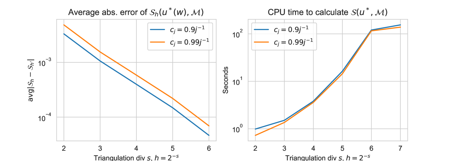
In our first test we compute a single reduced space $V$ using the greedy procedure on $\widetilde{\mathcal{M}}^{\mathrm{tr}}$. For each test candidate $u\in\widetilde{\mathcal{M}}^{\mathrm{te}}$ we calculate $u^{*}(P_{W}u)$. In Figure 2 we plot the difference between the coarse and fine surrogate distances $|\mathcal{S}_{h}(u^{*},\mathcal{M})-\mathcal{S}_{h^{\prime}}(u^{*},\mathcal{M})|$. We note that this error is significantly dominated by the calculated value of the estimator error (4), $\sigma_{\mathrm{est}}:=\mu(V,W)\,\varepsilon_{\mathrm{est}}(V,\mathcal{M})$ as we found $\sigma_{\mathrm{est}}\approx 10^{0}$ for $c_{j}=0.9j^{-1}$ and $\sigma_{\mathrm{est}}\approx 10^{1}$ for $c_{j}=0.99j^{-1}$. This dominates the errors presented in Figure 2 significantly.

Furthermore, we see a linear relationship in the right hand in Figure 2. The linear best fit of $\log(\mathrm{avg}_{\widetilde{\mathcal{M}}^{\mathrm{te}}}|\mathcal{S}_{h}-\mathcal{S}_{h^{\prime}}|)$ and $\log(h)=-s$ has slope $1.51$, which implies that on average

For the second test we examine the impact of using the coarse surrogate $\mathcal{S}_{h}(u^{*}_{k},\mathcal{M})$ for model selection. We build the $\sigma$-admissible families as outlined in §2 using the greedy splitting of $\mathcal{Y}=[-1,1]^{16}$. Note that at each point the cells $\mathcal{Y}_{k}$ are rectangular, which we can split in half in coordinate directions. We split the parameter space 7 times, resulting in $K=8$ local reduced spaces.

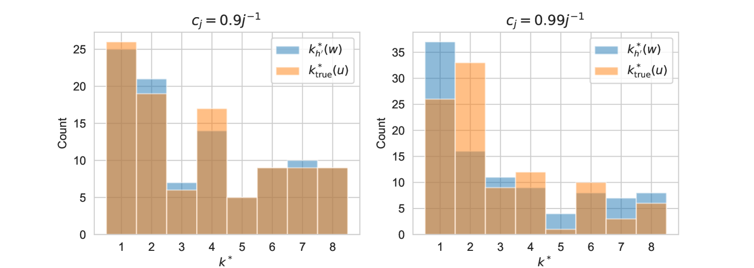
For each test candidate $u\in\widetilde{\mathcal{M}}^{\mathrm{te}}$ we have $K$ possible reconstructions $u_{1}^{*}(w),\dots u_{K}^{*}(w)$. We use the coarse surrogate in the model selection (9), writing $k^{*}_{h}(w)=k^{*}_{h}(P_{W}u)$ to make the dependence on $h$ and $w$ clear, and we inspect how often it agrees with the fine selection $k^{*}_{h^{\prime}}(w)$ for all test points $u$. We can also compare compare this to and the “true” selection $k^{*}_{\mathrm{true}}(u)$ for which $u\in\mathcal{M}_{k^{*}_{\mathrm{true}}}$.

Table 1 demonstrates that $k^{*}_{h}(w)$ agrees with $k^{*}_{h^{\prime}}$ the vast majority of the time from $h=2^{-4}$ onwards, in both cases for $c_{j}$. We also see that the fine selection $k^{*}_{h^{\prime}}$ agrees with the true selection 77 times out of 100 for $c_{j}=0.9j^{-1}$ and 64 times for $c_{j}=0.99j^{-1}$, that is, it picks the estimator $u^{*}_{k}(w)$ that is trained on the portion of manifold $\mathcal{M}_{k}$ that $u$ originated from. Out of interest we also plot the histogram of selections $k^{*}_{h^{\prime}}$ and $k^{*}_{\mathrm{true}}(u)$, recalling that they are a number in $1,\ldots,8$. We see broadly similar patterns in the reduced model selection. Given the CPU time savings that we see in Figure 2, we conclude that model selection through a coarse surrogate distance is a worthwhile numerical strategy.

References

- [1] Peter Binev, Albert Cohen, Wolfgang Dahmen, Ronald DeVore, Guergana Petrova, and Przemyslaw Wojtaszczyk. Convergence Rates for Greedy Algorithms in Reduced Basis Methods. SIAM Journal on Mathematical Analysis, 43(3):1457–1472, January 2011. Publisher: Society for Industrial and Applied Mathematics.
- [2] Peter Binev, Albert Cohen, Wolfgang Dahmen, Ronald DeVore, Guergana Petrova, and Przemyslaw Wojtaszczyk. Data assimilation in reduced modeling. SIAM/ASA Journal on Uncertainty Quantification, 5(1):1–29, 2017.
- [3] Albert Cohen, Wolfgang Dahmen, Olga Mula, and James Nichols. Nonlinear reduced models for state and parameter estimation. arXiv:2009.02687 [cs, math], November 2020. arXiv: 2009.02687.
- [4] Albert Cohen, Dahmen Wolfgang, Ronald DeVore, and James Nichols. Reduced basis greedy selection using random training sets. ESAIM: Mathematical Modelling and Numerical Analysis, January 2020.
- [5] Jan S. Hesthaven, Gianluigi Rozza, and Benjamin Stamm. Certified Reduced Basis Methods for Parametrized Partial Differential Equations. SpringerBriefs in Mathematics. Springer International Publishing, 2016.
- [6] Yvon Maday, Anthony T. Patera, James D. Penn, and Masayuki Yano. A parameterized-background data-weak approach to variational data assimilation: formulation, analysis, and application to acoustics. International Journal for Numerical Methods in Engineering, 102(5):933–965, May 2015.