Coexisting Hidden and self-excited attractors in an economic system of integer or fractional order
Abstract
In this paper the dynamics of an economic system with foreign financing, of integer or fractional order, are analyzed. The symmetry of the system determines the existence of two pairs of coexisting attractors. The integer-order version of the system proves to have several combinations of coexisting hidden attractors with self-excited attractors. Because one of the system variables represents the foreign capital inflow, the presence of hidden attractors could be of a real interest in economic models. The fractional-order variant presents another interesting coexistence of attractors in the fractional order space.
Keywords Hidden attractor; self-excited attractor; coexisting attractors; saddle; economic system
1 Introduction
According to Shilnikov criteria, chaos emergence requires at least one unstable equilibrium [Shilnikov(1965)]. So, if for some values of the key parameter the equilibria are unstable and one tries to generate attractors with initial conditions near these equilibria, one obtains chaotic attractors and could deduce that the system evolves chaotically. On the other side, this conclusion could be incomplete, or even false, since for initial conditions taken from an attraction basin which does not intersect with any small neighborhoods of unstable equilibria, the underlying trajectories could lead to some other attractor that might be a regular motion, but not a chaotic motion. Recently this problem has been managed by introducing the term of hidden attractor (see e.g. [Leonov & Kuznetsov(2013)], one of the first works on this subject, or [Kuznetsov(2015)]). If the attraction basin intersects with any open neighborhoods of an equilibrium the attractor is called self-excited, otherwise, it is called hidden. Usually, the self-excited attractors are numerically derived from unstable equilibria, while hidden attractors are difficult to be localized, because their attraction basins have no relation with small neighborhoods of any equilibria. Hidden attractors can be found in a nonlinear system with one or more stable equilibria [Molaie et al.(2013), Wang et al.(2017), Cang et al.(2019), Qigui et al.(2019)], with a line of equilibria (infinite equilibria) [Jafari & Sprott(2013)], with both unstable equilibria and stable equilibria [Danca(2017)], with coexistence of various attractors [Zhou et al.(2018)], or even without equilibria [Wei(2011)]. Note that there is a lack of correlation between hidden attractors and equilibria. Moreover, the precise localization of hidden attractors seems to be an intractable issue and, to our best knowledge, there is still no general analytical way, but only numerically with luck, to find hidden attractors (for the particular case of Chua’s circuit, see [Leonov et al.(2011)]).
To understand better the importance of hidden attractors consider the crash of aircraft YF-22 Boeing in April 1992. The analysis of aircrafts and launchers control systems with saturation regards the linear stability and also hidden oscillations which might occur [Andrievsky et al.(2013)]. The difficulties of rigorous analysis and design of nonlinear control systems with saturation related to this case are presented in [Lauvdal et al.(1997)].
Therefore, the identification of hidden attractors in a given system can help drive the system along the desired attractor, which can be a self-excited attractor or a hidden attractor.
The fractional order (FO) calculus is as old as the integer-order (IO) one, but its application was exclusive in mathematics. In the latter years FO systems where proved to describe, generally more accurately and in compact expressions, the behavior of real dynamical systems, compared to the IO models. This happens taking into account the nonlocal characteristic of “infinite memory”, i.e. the evolution of the system depends at each moment on the entire previous history. Basic aspects of the theory of FO can be found in [Oldham & Spanier(2006)]. While the definition of FO derivative for continuous-time real functions has been formulated by Liouville, Grunwald, Letnikov, and Riemann, in the late 19th century, the first definition of a fractional difference operator was proposed in 1974 [Diaz & Olser(1974)]. In this paper the FO derivative is considered in the sense of Caputo, because it allows the choosing initial conditions for the IO systems. One of the most utilized numerical methods to integrate continuous systems of FO is the predictor-corrector Adams-Bashforth-Moulton predictor-corrector method for fractional-order differential equations [Diethelm et al. (2002)].
There are many continuous but also discrete chaotic systems of IO, such as the supply and demand systems which are among the oldest and simplest economic discrete models, having complicated dynamics [Lorenz(1993)]. It is proved that the economical models exhibit generally unstable steady states and also fluctuations if the income distribution varies sufficiently and if shareholders save more than workers (see e.g. [Miloslav(2001)] and references therein).
In this paper a continuous economic system is considered, and proved numerically that it presents coexisting attractors for both IO and FO variants.
2 The economic system
In [Miloslav(2001)] the question of whether using and/or un-using of foreign investments can change the qualitative properties is addressed for a growth path of a proposed dynamical economic system with three endogenous variables and only one non-linear term, modeled by 3-dimensional autonomous differential equations, while in [Pribylova(2009)] the system is further analyzed via bifurcations routes including supercritical and subcritical Hopf bifurcation, and generalized Hopf bifurcation as well. It is proved that the existing cycle exhibits period-doubling bifurcation as a route to chaos.
The economic system considered in this paper, with a foreign financing, has the following form
| (1) |
where the variables represents the savings of households, the Gross Domestic Product (GDP), the foreign capital inflow, and the variables the variation of the marginal propensity to savings, the ratio of capitalized profit, the potential GDP, , with the capital/output ratio, the capital inflow/savings ratio and the debt refund/output ratio [Lorenz(1993)]. As explained in [Lorenz(1993)], if , the activities are not constrained and high profits are derived from the sectors where the markets are not yet saturated. The single non-linearity represents the quality of a capitalization of the profits. If , then the inflation is possible. A lack of new investment opportunities modifies it by savings.
Note that the system can also be viewed as an extension of the van der Pol s system on the plane , i.e. when economically the system has no foreign investment ()
| (2) |
which, as a two-dimensional autonomous system, cannot display chaotic behavior.
In this paper one considers the 3-dimensional system (1) with the bifurcation parameter and , , , , (there are other interesting possible parameters choices111Parameter has been chosen as in [Miloslav(2001)], with six decimals, because rounding to fewer decimals affects significantly the results.)
| (3) |
While in [Miloslav(2001)] coexisting stable cycles and equilibria and also the existence of a chaotic attractor are studied analytically, in this paper it is shown numerically that for the system presents richer dynamics, including coexisting hidden and self-excited chaotic attractors and stable cycles. This behavior could be extremely interesting from an economical point of view.
Because the right hand side of the system (1) is an odd function, the system presents symmetries in the bifurcation planes, and also in the phase space.
The equilibria, which are collinear (see Fig. 4), have the following expression
Note that with the considered 4 decimals, are approximations of the exact equilibria .
The stability of equilibria and the occurrence of the Hopf bifurcation for are studied in [Miloslav(2001)].
In this paper, the bifurcation parameter is considered, , where all equilibria are unstable and the system presents most interesting dynamics.
The following result, presented in [Miloslav(2001), Pribylova(2009)], is slightly improved and re-proved numerically here, to be useful for finding hidden attractors later.
Lemma 1.
[Miloslav(2001), Pribylova(2009)] For , equilibria are hyperbolic unstable saddles. Equilibrium is attracting focus-saddle and repelling focus-saddle.
Proof.
The stability is proved numerically by analyzing the eigenvalues of the Jacobi matrix which has the following form
-
i)
The characteristic equation , , where is the characteristic polynomial, for , has the following form
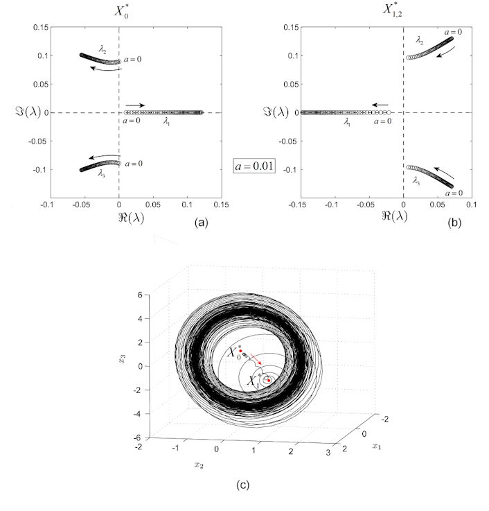
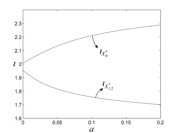
Because, for , the coefficient and there exists a single change in the sign of the coefficients of . Therefore, by Descartes rule, there exists a single real positive zero of , . For , the coefficient and the coefficients sign are: , i.e. three sign changes, which means that the polynomial has either 3 or 1 positive zeros. In order to understand better the characteristics of , in Fig. 1 (a) the three roots of , , are plotted as function of , for . As can be seen, the real eigenvalue is positive for all considered values of and the other two eigenvalues are complex with . Therefore, is spiral saddle of index 1 (or attracting focus saddle). This means that trajectories will leave this equilibrium along the unstable manifold of dimension 1 (generated by the real positive eigenvalue ), by spiralling, due to the stable manifold of dimension 2 (generated by ).
-
ii)
For equilibria , the characteristic polynomial is
The proof of instability of , via Hurwitz stability criterion, can be found in [Miloslav(2001)]. To verify it numerically, in Fig. 1 (b) the zeros of are plotted as function of for . As can be seen, for all , there exist two complex eigenvalues with positive real parts and one real negative eigenvalue. Therefore are spiral saddle of index 2 (or repelling focus saddle). Trajectories near are attracted along the stable manifold of dimension 1 (generated by the real negative eigenvalue ) and then are rejected spiraling on the unstable manifold of dimension 2 (due to the positiveness of the real part of , ).
-
iii)
Because for all equilibria , , are hyperbolic.
∎
Fig. 1 (c) presents a chaotic attractor for . As can be seen, before reaching the chaotic attractor, the trajectory connects the saddles and , i.e. it is a heteroclinic connection.
3 Hidden and self-exited attractors
Hereafter attractors are denoted as follows:
-
Self-Excited Cycles: ;
-
Self-Excited Chaotic Attractors: ;
-
Hidden Chaotic Attractors: ;
-
Hidden Cycles: .
The numerical method utilized for the integration of the system (3) of IO is the Matlab variant of RK method, .
The numerical trajectories for different attractors are represented overplotted in the phase space, as time series and the local Lyapunov exponents are determined. Generally, transients are removed. Also, excluding the Perron effect (when a negative largest Lyapunov exponent does not, in general, indicate stability, and also when a positive largest Lyapunov exponent does not, in general, indicate chaos [Perron(1930), Leonov & Kuznetsov(2007)]), the positiveness of the maximal Lyapunov exponent (MLE) is considered as an evidence for chaos. In this paper the zero MLE is considered as having a maximum value of order . If is zero, then, after transients removed, the trajectory is considered as regular (stable cycle), while if the trajectory is considered chaotic.
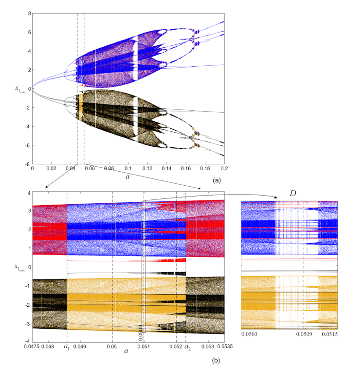
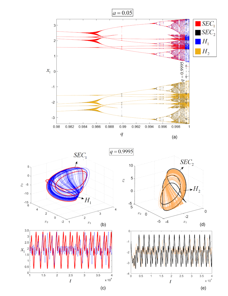
The bifurcation diagram of the maximum component , for , is presented in Fig. 2 (a).
As can be seen, for all values of , the underlying attractors are symmetric. Due to the symmetry, the coexistence of attractors features this system. Thus, depending on the initial condition , there exists one or even two pairs of symmetric attractors (blue-red and black-yellow in the bifurcation diagram). Beside the standard period-doubling cascade which leads to chaos, the zoomed region in Fig. 2 (b) reveals an interesting coexisting window for , with and , where exterior and interior attractors crises, thin periodic windows interleaved between large coexisting chaotic-periodic windows, and also several miniature bifurcation diagrams within a large chaotic window can be seen. Moreover, at , there exist both exterior and interior crisis.
However the most interesting characteristic of the window presented in Fig. 2 (b) represents the coexistence of self-excited chaotic attractors with hidden chaotic attractors.
Because there exists no general analytical way to find the attraction basin of hidden attractors of a given nonlinear system, in the case when the considered system admits unstable equilibria, an acceptable way is to search randomly initial conditions in neighborhoods of all these equilibria. This can be done either in planar (usually horizontal) sections through each equilibrium or/and analyzing three-dimensional (usually spherical) neighborhoods centered on equilibria.
For the considered system (3), one considers lattices of points and zoomed regions, as horizontal sections through (with ) and (with the third coordinate of ), respectively, and also spherical neighborhoods of unstable equilibria.
Because of the symmetry, the case of the equilibrium is similar to . Therefore only and are analyzed.
3.1 Coexisting self-excited chaotic attractors and hidden chaotic attractors
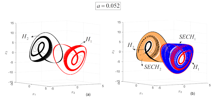
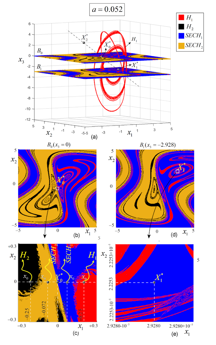
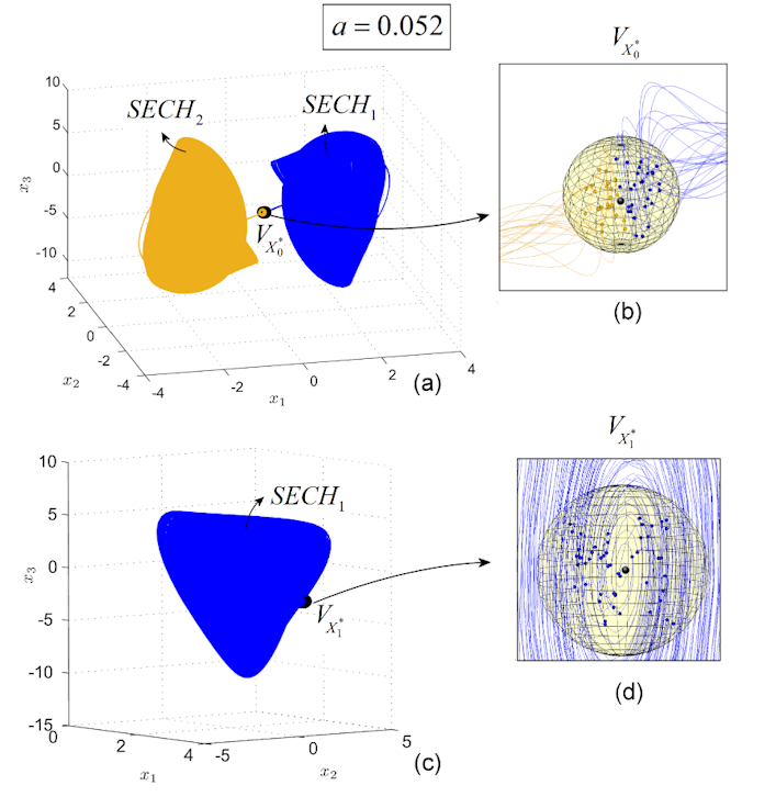
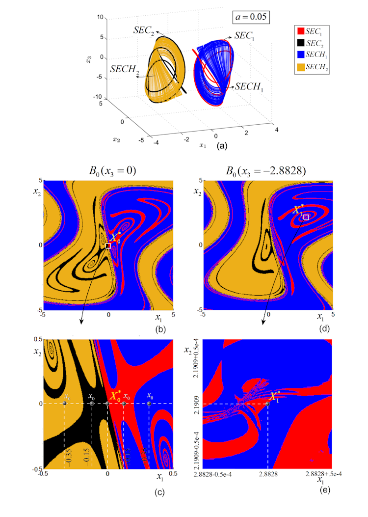
. For this value, and the system presents two pairs of different chaotic attractors, , and , respectively (see Fig. 3 (a) for and and Fig. 3 (b) for both pairs of hidden attractors and self-excited attractors). The extensive numerical experiments revealed that initial conditions within small neighborhoods of unstable equilibria and launch trajectories to self-excited chaotic attractors (blue and light brown). Initial conditions outside the attraction basins of the self-excited attractors lead to the other two chaotic attractors, (red and black), which are hidden chaotic attractors. To verify that, one can explore planar neighborhoods of each equilibria in lattices , containing and defined by , and , containing and defined by (Fig. 4 (a)). All points in are considered as initial conditions, to see where the underlying trajectories go. As the numerical analysis shows, the attraction basins of and on do not contain (intersect) the equilibrium (see the black and red plot in Figs. 4 (b), (c)). Similarly, these attraction basins do not intersect the equilibrium on (Figs. 4 (d), (e)). Therefore are hidden attractors.
Note that is on the separatrix between the attraction basins of and and, therefore, every (no matter how small) neighborhoods around (Fig. 4 (c)) share initial conditions toward or . This situation is typical for this system and also for saddles generally. Therefore, are self-excited.
In addition to planar numerical analysis, a three-dimensional test around and is done by analyzing initial conditions within a sphere surrounding these equilibria. For clarity, 50 random points as initial conditions are chosen. Figs. 5 (a), (b) presents the case of equilibrium with the neighborhood . As can be seen, due to the fact that is placed on the separatrix, the neighborhood shares initial conditions for attractors and .
In Figs. 5 (c), (d), within a spherical neighborhood , 50 initial conditions are all leading to .
Therefore, because the chaotic attractor is not connected with any equilibria and , it can be considered hidden.
The self-excited attractors have , while for the attractors , and, therefore, they are chaotic.
3.2 Coexisting self-excited cycles and self-excited chaos
. Within the window (Fig. 2 (b)), as the bifurcation diagram shows, there exists a pair of symmetric stable cycles (red and black in Fig. 6) coexisting with a pair of symmetric chaotic attractors (blue and light-brown). Similar numerical approach to the one discussed in Subsection 3.1, shows that for and , there exists a pair of stable cycles, and (red and black plot, Fig. 6 (a)) and of chaotic attractors and (blue and light-brown).
Consider the lattices (Figs. 6 (b) and (c)) and (Figs. 6 (d) and (e)) in the planar sections through and . As for the case , belongs to a separatrix between attraction basins of and (Fig. 6 (c)) and, therefore, are self-exited attractors. The zoom in Fig. 6 (e) shows the fact that for this value of , also belongs to the separatrix of attraction basins of and (red and blue respectyively, Fig. 6 (d), (e)), confers the status of self-excited characteristic of these attractors.
Even by considering that attraction basins of do not intersect (blue and light-brown in Fig. 6 (c)), they can be hidden, because of the position of , (red in Fig. 6 (e)) are actually not hidden.
Note that with an extremely small perturbation of , , from the previous case of , the attraction basins suffered significant modifications around , so that the hidden characteristic vanished.
The attractors have and, therefore, are stable cycles. For , , i.e. these attractors are chaotic.
3.3 Coexisting self-excited cycles and hidden cycles
. The zoomed region defined for (Fig. 2 (b)) contains merged periodic and chaotic thin windows. Within these interesting windows, one can identify the coexistence of several types of possible periodic attractors. The uncertainty relates to thickness of these windows, to the six decimals of some coefficients of the system and also to the errors introduced by the numerical integration. Also, the regularity seems to be influenced by the close proximity of the periodic windows with thin chaotic bands.
To increase the precision of the integration, in the build-in Matlab procedure ode45, the option is used (the default relative tolerance of ode45 integrator, , cannot separate, in a reasonable time integration interval , the chaotic transients from the stable cycles).
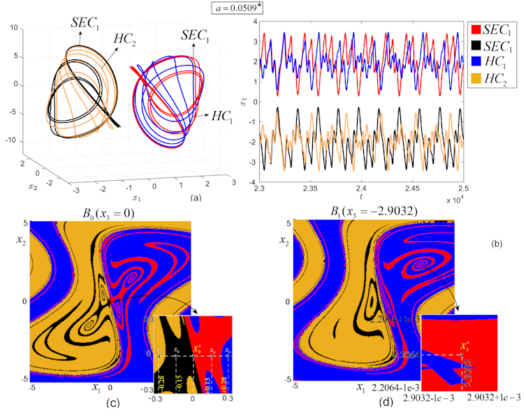
For , because of the mentioned utilized , the equilibria become , and there exist two pairs of stable cycles: self-excited cycles and (red and black in Fig.7 (a)) and hidden cycles and (blue and light-brown). The presumed stability can be deduced from the time series in Fig. 7 (b), while the type of attractors can be deduced as before from the sections through equilibria , the lattice through (Fig. 7 (c)) and through (Fig. 7 (d)).
Again, a small perturbation of the bifurcation parameter with only (from to ), generates a modification in the attraction basins containing (compare Fig. 7 (d) with Fig. 6 (d)), so that the hiddenness property appeared again.
For both pairs of cycles, .
4 FO variant of the system (3)
Probably the most interesting characteristic of this system is the coexistence of attractors in the space of the fractional-order systems in the sense that for some fractional order and fixed parameter , there exist two symmetric pairs of coexisting chaotic and stable cycles attractors.
The commensurate FO variant of the system is
| (4) |
where denotes the Caputo differential operator of order with starting point 0 (see e.g. [Podlubny(1999), Diethelm et al. (2002)])
where denotes the ceiling function that rounds up to the next integer and represents the standard differential operator of order . Due to the use of Caputo’s operator, the initial conditions can be taken as for the integer-order case.
Lemma 2.
For , equilibria and are unstable.
Proof.
In order to study the stability of equilibria and of the system (4), denote , for , where are the arguments of the eigenvalues. The stability theorem of equilibria of a FO system can be stated in the following practical form
Theorem 1.
[Tavazoei & Haeri(2008), Danca(2017)] An equilibrium point is asymptotically stable if and only if the instability measure
is strict negative.
If and the critical eigenvalues satisfying have geometric multiplicity one, is stable.222The geometric multiplicity represents the dimension of the eigenspace of corresponding eigenvalues.
The graphs of for all equilibria, with , are presented in Fig. 8. As can be seen and, therefore, equilibria are unstable. ∎
Consider next . The bifurcation diagram with respect the fractional order is presented in Fig. 9 (a). As can be seen, at the right of the bifurcation diagram, there exists a FO coexisting window where two symmetric pairs of attractors coexist.
Remark 3.
Generally for FO systems, attractors coexisting phenomenon is searched for a fixed fractional order in the parameter bifurcation space, by searching different initial conditions for some fixed parameter value. For this system of FO the coexistence of attractors can be found also in the fractional order space, by searching for initial conditions for a fixed parameter bifurcation.
Note that, as for continuous integer-order systems and contrary to FO difference systems, where the chaos strongness decreases for increasing (see e.g. [Danca(2020)]), for this system of FO, the chaos strongness increases with tending to 1.
Because the inherent time history of the ABM method, a deep numerical analysis to detect hidden attractors is tedious and time consuming. Therefore, the quality of the obtained attractors is determined by several empirical tests.
, a value within the coexisting window (Fig. 9 (a)). Equilibria are the same as for the IO case, for , namely . The two symmetric pairs of FO-attractors are presented in Figs. 9 (b), (c) and Figs. 9 (d), (e) (phase portraits and time series, respectively). As can be seen, each pair of FO-attractors is composed by one self-excited cycle, or (red and black respectively) and one hidden chaotic attractor or (blue and light-brown, respectively).
Now, the cycles have while for the chaotic attractors .
Therefore, for a given parameter value , the FO system (4) admits at least one FO coexisting window in the space of fractional order , with two symmetric pairs of coexisting attractors. Other potential FO-coexisting windows, not examined here, are at the bifurcation points, e.q. at about .
This important characteristic indicates that for some given fractional order and parameter , there could be two different systems.
5 Numerical settings
Choosing a suitable level of precision for computations is a real challenging task. The numerical integrator for (3) in the IO case is the matlab ode45 with implicit absolute and relative error tolerances. For the particular case of (Subsection 3.3), errors have been reduced by using .
The maximal time used interval is , depending on the lengths of discarded transients. Due to inherent numerical errors, larger values for could lead to invalid results.
To integrate numerically the system (4) of FO, the ABM method [Diethelm et al. (2002)] is utilized.
The algorithms used to determine the finite time MLEs are the Benettin-Wolf algorithm for the IO case, and the algorithm presented in [Danca & Kuznetsov(2018)] for the FO case.
The attractors data are presented in Table 1. Beside the initial conditions presented in Table 1, points and can be used as initial conditions.
Note that, because of the relatively large number of decimals of some system coefficients and also due the inherent numerical errors, the 4-digits coordinates of (as approximations of the exact ) could also be taken as initial conditions, for cases with neighborhoods of .
Conclusion and Discussion
In this paper several type of coexisting attractors of an economic system of IO and FO are presented. Considering one of the several parameters as bifurcation parameter, the bifurcation diagram revealed windows where hidden and self-excited attractors coexist.
First, it is shown numerically that equilibria are unstable for both IO and FO cases, after which the exploration within neighborhoods of these points is investigated. The experiments, realized with the matlab routine ode45 for the IO case and with the ABM method for the FO case, show that the considered attractors fit the definition of hidden or self-excited attractors.
The characteristics of chaotic or regular attractors are revealed, after transients removed, by phase portraits, time series and maximal Lyapunov exponents.
For the bifurcation diagram in Fig. 1, the four used initial conditions are and , respectively. These initial conditions are proved to be valid, besides those mentioned in the text, for all considered cases (Table 1). Nevertheless, to note that generally this is a way to draw bifurcation diagrams are made for fixed initial conditions, it is not a rigorous method, since the attraction basins be modified while the bifurcation parameter varies. Thus some searched attraction basins, such as hidden attractors, might modify once the parameter is varied and, in this way, hidden attractors can “hide” from this searching method. Indeed, one can consider as initial approximations of unstable equilibria (if any), whose expressions depend on parameter, which will lead certainly to all self-excited attractors (if any). But, the chance to identify in this case hidden attractors diminishes significantly. Moreover, sudden changes in the bifurcations branches may indicate bifurcations when some branches may become unstable, but also they might be due to the mentioned dependence of the attraction basins with the parameter modification, when the bifurcation diagram is incomplete. For example, for this system of IO, for values of close to , with relative small perturbations of , of order of or even of (case and ), the attraction basins change their properties related to hiddenness and self-excited.
A coexisting window in the space of fractional order indicates that analyzing a FO system by following only the bifurcation in the parameter space, without some analysis of the bifurcation diagram in the fractional order space, could be insufficient to identify the entire spectrum of system dynamics.
An important problem, for this system, is a deeper analysis of his FO variant.
The coexistence of attractors in the case of this system is influenced by the presence of the saddles on the separatrix of attraction basins. For all these cases, when the unstable manifolds of the saddle could separate the attraction basins (see the cases in Fig. 4 (c), Figs. 6 (c) and (e) and Fig. 7 (c)), this problem could be analyzed further as a possible sufficient criterion for non-existence of hidden attractors.
Because the variable represents the foreign capital inflow [Miloslav(2001)], the presence of hidden attractors could represent an important phenomenon from the economic point of view. In fact under some circumstances such as initial conditions, the dynamics of the system could cover some (hidden) behavior. Also, counterintuitively, due to the existence of hidden attractors, increasing (but also decreasing) the variable is not necessarily related with the system economical stability.
References
- [Shilnikov(1965)] Shilnikov, L.P. [1965] “A case of the existence of a denumerable set of periodic motions,” Dokl. Akad. Nauk SSSR 160(3), 558 561.
- [Leonov & Kuznetsov(2013)] Leonov, G.A. & Kuznetsov, N.V. [2013] “Hidden attractors in dynamical systems: from hidden oscillation in hilbert-kolmogorov, Aizerman and Kalman problems to hidden chaotic attractor in chua circuits,” Int. J. Bifurcat. Chaos 23(1), 1330002.
- [Kuznetsov(2015)] Kuznetsov, N.V. [2015] “Hidden Attractors in Fundamental Problems and Engineering Models: A Short Survey,” Lecture Notes in Electrical Engineering, 371, 13-25 (Springer, Switzerland).
- [Molaie et al.(2013)] Molaie, M., Jafari, S., Sprott, J.C., & Golpayegani, S.M.R.H. [2013] “Simple chaotic flows with one stable equilibrium,” Int. J. Bifurcat. Chaos 23(11), 1350188.
- [Wang et al.(2017)] Wang, X., Pham, V.T, Jafari, S., Volos, C., Munoz-Pacheco, J.M., & Tlelo-Cuautle, E. [2017] “A new chaotic system with stable equilibrium: From theoretical model to circuit implementation,” IEEE Access 5, 8851-8858.
- [Cang et al.(2019)] Cang, S., Li, Y., Zhang, R., & Wang, Z. [2019] “Hidden and self-excited coexisting attractors in a Lorenz-like system with two equilibrium points,” Nonlinear Dyn. 95(1), 381-390.
- [Qigui et al.(2019)] Qigui, Y., Yang, L., Ou, B. [2019] “Hidden Hyperchaotic Attractors in a New 5D System Based on Chaotic System with Two Stable Node-Foci,” Int. J. Bifurcat. Chaos 29(7), 1950092.
- [Jafari & Sprott(2013)] Jafari, S., Sprott, J.C. [2013] “Simple chaotic flows with a line equilibrium,” Chaos Solitons Fractals 57, 79-84.
- [Danca(2017)] Danca, M.F. [2017] “Hidden chaotic attractors in fractional-order systems,” Nonlinear Dyn., vol. 89(1), 577-586.
- [Tavazoei & Haeri(2008)] Tavazoei, M.S. & Haeri, M. [2008] “Chaotic attractors in incommensurate fractional order systems,” Phys. D 327(20), 2628 2637
- [Zhou et al.(2018)] Zhou, W., Wang, G.Y., Shen, Y.R., Yuan, F., & Yu, S.M. [2018] “Hidden coexisting attractors in a chaotic system,” Int. J. Bifurcat. Chaos 28(10), 1830033.
- [Wei(2011)] Wei, Z. [2011] “Dynamical behaviors of a chaotic system with no equilibria,” Phys. Lett. A 376(2), 102-108.
- [Leonov et al.(2011)] Leonov, G.A., Kuznetsov, N.V., & Vagaitsev, V.I. [2011] “Localization of hidden Chua’s attractors,” Phys. Lett. A 375(23), 2230-2233.
- [Andrievsky et al.(2013)] Andrievsky, B.R., Kuznetsov, N.V., Leonov, G.A., & Pogromsky, A.Y. [2013] “Hidden os-cillations in aircraft flight control system with input saturation,” IFAC Proceedings Volumes (IFAC-PapersOnline) 46(12), 75-79.
- [Lauvdal et al.(1997)] Lauvdal, T., Murray, R., Fossen, T. (1997] “Stabilization of integrator chains in thepresence of magnitude and rate saturations: a gain scheduling approach,” In:Proc. IEEE Control and Decision Conference. 4, 4404-4005.
- [Oldham & Spanier(2006)] Oldham, K.B., Spanier, J. [2006] The Fractional Calculus: Theory and Applications of Differentiation and Integration to Arbitrary Order. (Dover Publication, Mineola).
- [Diaz & Olser(1974)] Diaz, J.B., Olser, T.J. [1974] “Differences of fractional order,” Math. Comput. 28(125), 185-202.
- [Diethelm et al. (2002)] Diethelm, K., Ford, N.J., Freed, A.D. [2002] “A predictor-corrector approachfor the numerical solution of fractional differential equations,” Nonlinear Dyn. 29, 3-22.
- [Lorenz(1993)] Lorenz, H.W. [1993] Nonlinear Dynamical Economics and Chaotic Motion 2nd ed (Springer-Verlag, Berlin).
- [Miloslav(2001)] Miloslav, V. [2001] “Bifurcation Routes And Economic Stability,” Bulletin of the Czech Econometric Society 8.
- [Pribylova(2009)] Pribylova, L. [2009] “Bifurcation routes to chaos in an extended van der Pol’s equation applied to economic models,” The Electron. J. Differ. Equat. 53, 1-21.
- [Perron(1930)] Perron, O. [1930] “Die Stabilitatsfrage bei differentialgleichungen,” Mathematische Zeitscrift, 32,702-728.
- [Leonov & Kuznetsov(2007)] Leonov, G.A. & Kuznetsov, N.V. [2007] “Time-varying linearization and the Perron effects,” Int. J. Bifurcat. Chaos, 17(4), 1079-1107.
- [Podlubny(1999)] Podlubny, I. [1999] Fractional Differential Equations (Academic Press, San Diego).
- [Danca(2020)] Danca, M.F. [2020] “Puu system of fractional order and its chaos suppression,” Symmetry 12(3), 340.
- [Danca & Kuznetsov(2018)] Danca, M.F., Kuznetsov, N. [2018] “Matlab code for Lyapunov exponents of fractional order systems,” Int. J. Bifurcat. Chaos 28(05), 1850067.