Coherent post-ionization dynamics of molecules based on adiabatic strong-field approximation
Abstract
Taking N2 and O2 as examples, we theoretically study the post-ionization dynamics of molecules in strong laser fields using a density matrix method for open systems, focusing on the effect of ionization-produced coherence on the dynamics of residual ions. We introduce the adiabatic strong-field approximation (ASFA) method to predict the coherences between ionic states resulting from multiorbital strong-field ionizations. Compared with the standard SFA, the ASFA method can be applied across a wide range of laser intensities due to the consideration of orbital distortion effects. Based on the ASFA, it is found that there are obvious coherences between ionic states in residual molecular ions. These coherences significantly influence the transitions between ionic states, which finally change the post-ionization dynamics of molecular ions. Our findings reveal the importance of the ionization-produced coherences in modulating post-ionization molecular dynamics.
I INTRODUCTION
When molecules are exposed to intense laser pulses, strong-field ionizations from multiple molecular orbitals (MOs) could create coherent superpositions of ionic states McFarland et al. (2008); Smirnova et al. (2009); Pabst et al. (2016). These coherences can induce oscillatory charge migration, the frequency of which is determined by the energy gap between ionic states Goulielmakis et al. (2010); Wirth et al. (2011); Kraus et al. (2013); Calegari et al. (2014). Driven by electron-nuclear interactions, the electron motion subsequently triggers atomic rearrangements within the molecule on femtosecond to picosecond timescales Breidbach and Cederbaum (2003, 2005); Belshaw et al. (2012); Hennig et al. (2005); Wörner et al. (2017). Revealing the mechanisms of coherence generation during strong-field ionization and its impact on the dynamics of the residual molecular ions is crucial for comprehending strong-field post-ionization phenomena, which ultimately paves the way for coherent control in biochemical reaction processes.
To theoretically investigate the post-ionization molecular dynamics, one should consider both the multi-electron effect and the nuclear motion. This makes the utilization of the full-dimensional time-dependent Schrdinger equation (TDSE) impractical. So far, full-dimensional TDSE calculations for molecules have been constrained to small molecules like H2 Palacios et al. (2006); Ishikawa and Sato (2015). Ab-initio calculations for more complex molecular systems remain scarce Vacher et al. (2017). To address this issue, an open-system density matrix (DM) method has been developed recently Chen et al. (2019); Zhang et al. (2020); Lei et al. (2022); Yuen and Lin (2022); Yuen et al. (2023). By incorporating the ionic reduced DMs (RDMs) generated by instantaneous strong-field ionizations of parent molecules into the DM equations (see Eq. (15)), the strong-field ionization, electric dipole coupling, and nuclear motion could be treated on equal footing in principle. To date, open-system DM methods primarily incorporate the ionic state populations generated by strong-field ionizations Chen et al. (2019); Zhang et al. (2020); Lei et al. (2022). The off-diagonal terms, namely the ionization-produced coherences, have not been adequately addressed. Despite this, theoretical simulations still qualitatively reproduce experimental results Chen et al. (2019); Zhang et al. (2020); Lei et al. (2022); Zhang et al. (2020); Lei et al. (2022). In fact, laser ionizations can produce coherences in the residual ions. For atomic systems, the electronic coherences produced by photoionization and strong-field ionization have been studied Rohringer and Santra (2009); Pabst et al. (2016); Carlström et al. (2017). But for molecules, the situation becomes more complicated due to nuclear motions. Several studies focus on the coherence evolution in polyatomic molecular ions produced by single-photon ionization. It has been found that the electronic coherence typically decays over a timescale of a few to hundreds of femtoseconds due to the dephasing and the decreased overlap of the nuclear wavepacket Vacher et al. (2015); Arnold et al. (2017); Vacher et al. (2017). However, for molecules ionized by strong-field ionization, the generation of coherences within the residual ions has not been adequately studied. Moreover, the influence of the coherence on the dynamics of molecular ions remains unclear.
Based on the strong-field approximation (SFA), Pabst et al. proposed an intuitive approximative method that effectively predicted the coherence produced by strong-field ionization in xenon atoms Pabst et al. (2016). Recently, we extended this method to diatomic molecular systems and verified its validity on a one-dimensional H2 system Xue et al. (2021). This method has also been used to explain the abnormal ellipticity dependence of N air lasing Zhu et al. (2023). In this work, we refer to it as the “Simple” method. Recently, Yuen et al. developed an alternative approximative method based on partial wave expansion (PWE) Yuen and Lin (2023). At the lowest order of the weak field asymptotic theory, the ionization amplitudes of partial waves are calculated, enabling the prediction of the ionic RDM Tolstikhin et al. (2011). This method achieves the same level of accuracy as the molecular Ammosov-Delone-Krainov (MO-ADK) theory in calculating the tunnelling ionization rate Tong et al. (2002); Zhao et al. (2010). However, symmetry analysis suggests that ionizations from MOs with opposite parity should not generate coherence between the resulting ionic states. This contradicts the expectations of both the “Simple” and the PWE methods, indicating that the generation of ionic coherences in molecules upon strong-field ionization remains elusive.
In this work, we investigate the ionic coherences generated by strong-field ionizations using the adiabatic strong-field approximation (ASFA), which is a combination of the SFA and the adiabatic field-distorted MOs. In Refs. Śpiewanowski et al. (2013); Śpiewanowski and Madsen (2014, 2015), it has been used to study the strong-field ionization and high-order harmonic generation of molecules. These works highlight the potential importance of orbital distortion in explaining experimental phenomena. For molecular systems, coherences can be classified as vibrational coherence and vibronic coherence. By using the ASFA, we find that the coherence between ionic states with opposite parities can be produced by strong-field ionization, which can not be captured by the standard SFA. Moreover, both of these coherences can influence the transitions between ionic states within the residual ions. Ultimately, the post-ionization dynamics of molecular ions are changed by these ionization-produced coherences.
The paper is structured as follows. In Sec. II, we provide a brief review of the “Simple” and PWE methods and introduce the (A)SFA method. We then present the open-system quantum Liouville equations. In Sec. III, using N2 and O2 as examples, we investigate the properties of ionization-produced coherences and their roles in post-ionization molecular dynamics. Section IV provides a summary. Atomic units are used throughout unless indicated otherwise.
II THEORETICAL METHODS
For a molecule with electrons, the ionized molecular system can be described as an entangled state composed of the ion and the free electron at the instant of ionization. The state can be expressed as
| (1) |
Here, represents the -th ionic bound state generated by the ionization of the -th MO in the neutral molecule. It is approximated using a Slater determinant. represents the wavefunction of the resulting ionized electron with the momentum , approximated as a plane wave. is the antisymmetrizing permutation operator on the -th and -th electron coordinates. is the instantaneous ionization amplitude. Note that describing a molecular bound state using a single Slater determinant becomes inaccurate when electronic correlation effects are significant. To address this issue, one can adopt the density functional theory (DFT), which, in principle, incorporates both exchange and correlation effects. Alternatively, one can use more advanced post-HF methods, where the bound-state wavefunction is no longer restricted to a single Slater determinant.
In the basis set of ionic bound states, the ionic RDM produced by instantaneous ionization can be calculated by tracing out the free electrons, and is given by
| (2) |
The diagonal terms represent the ionization rates from the neutral state to different ionic states. The off-diagonal terms represent the instantaneous ionization-produced coherences.
II.1 “Simple” method
In the “Simple” method, we denote the free electron wavepacket transiently ionized from the -th molecular orbitals (MOs) as . It is assumed that the free-electron wavepackets ionized from different MOs share the same waveform Pabst et al. (2016); Xue et al. (2021), differing only by a complex coefficient . This coefficient depends on the angle between the molecular axis and the field direction, the binding energy, and the wavefunction of the ionizing MO. Using a plane wave expansion, it means , where is the ionization amplitude. Following Eq. (2), the instantaneous ionization-produced RDM reads
| (3) | ||||
In the final step of the derivation, we utilize the equality condition in the Cauchy-Schwarz inequality, because and are linearly dependent. Strictly speaking, the assumption that and share the same waveform is too restrictive, and should depend on . According to the Cauchy-Schwarz inequality, the exact value of should be smaller than . This indicates that the off-diagonal elements, namely the instantaneous ionization-produced coherences, calculated using the “Simple” method, are somewhat overestimated.
In the following, we determine the phase difference through a simple derivation. For homonuclear diatomic molecules, the MO wavefunction has a definite even () or odd () parity. For the orbital, the transition dipole moment (TDM) is a function of . Given that the instantaneous ionization amplitude ( is the electric field along the space axis), and strong-field ionization primarily occurs in the opposite direction of the electric field, one obtains for a MO and for a MO. Therefore, when two ionizing MOs possess the same parity, . When they possess opposite parity, . Hence, the exponential term in Eq. (3) can be further written as . Here, sgn is the sign function. describes the parity of the -th ionizing MO, with a value of for parity. By replacing with the MO-ADK ionization rate Tong et al. (2002); Zhao et al. (2010), Eq. (3) can be rewritten as
| (4) |
Considering the free evolution of the ionization-produced RDM, the RDM at a final time can be given by
| (5) | ||||
The same equation can also be found in Ref. Pabst et al. (2016), differing only by the constant term , which has no substantial impact on the results.
II.2 Partial-wave-expansion method
Based on the weak-field asymptotic theory and PWE Tolstikhin et al. (2011); Song et al. (2023), Yuen et al. proposed an alternative method to calculate the ionization-produced RDM Yuen and Lin (2023),
| (6) |
Here, is the partial ionization amplitude from the -th ionizing orbital. is the magnetic quantum number along the space axis. Using the adiabatic approximation, is expressed as
| (7) | ||||
where with being the ionization potential of the -th ionizing orbital. is the effective asymptotic charge experienced by the ionized electron. Considering that the electron is ionized in the opposite direction of the electric field , can be given by
| (8) |
where
| (9) |
Here, is the structure parameter of the -th ionizing orbital Zhao et al. (2010). is the orbital angular momentum quantum number. is the magnetic quantum number along the molecular axis. represents the Wigner D-matrix for rotating the molecule. Notably, this method aligns with the MO-ADK theory for calculating ionization rates, which allows for the computation of tunnelling ionization rates from MOs at different molecular axis angles.
II.3 Adiabatic strong-field approximation method
In this section, we introduce the ASFA coherence method. In the length-gauge SFA, the amplitude for producing an ion in the -th state, accompanied by a free electron with the momentum at the end of the laser field , is given by Pabst et al. (2016); Śpiewanowski and Madsen (2014)
| (10) |
Here, is the TDM element from the ionizing MO to the plane wave . with being the vector potential of the laser field. is the time-dependent eigenenergy of the -th MO. In the adiabatic approximation, the laser field at the ionization instant can be treated as a static electric field. This treatment results in the distortions of MOs. Then the eigenequation for the MO becomes
| (11) |
Here, is the effective one-electron Hamiltonian operator, which is composed of the field-free Hamiltonian and the interaction term . In this work, adiabatic MOs are computed using the DFT as implemented in the GAUSSIAN16 program package Frisch et al. . We adopted the B3LYP exchange-correlation functional and the augmented correlation-consistent polarized valence quadruple-zeta (aug-cc-pVTZ) basis set. The basis set incorporates diffuse functions, which can effectively characterize the field-induced diffusion of MOs.
By tracing out the degrees of freedom of the ionized electron, we obtain the RDM of the ion
| (12) |
Substituting Eq. (10) into the equation above and assuming that electron wavepackets with the same but emitted at different times have negligible overlap due to rapid wavepacket spreading, this allows us to determine the coherence by neglecting the terms where two ionic states are populated at different times Pabst et al. (2016). As a result, Eq. (12) can be simplified as
| (13a) | ||||
| (13b) | ||||
Here, is the RDM of the ion at the end of the laser pulse, when dipole transitions between ionic states are excluded. represents the instantaneous ionic RDM generated at time . To consider dipole transitions between ionic states, we can incorporate into the open-system DM equation that describes the evolution of the ion system. To assess the degree of coherence (DOC) of the ion generated by instantaneous ionization, we define
| (14) |
as the complex DOC. It contains both the DOC and the phase information of the coherence. Since can be obtained using either SFA or ASFA, the superscript “A” refers to either “SFA” or “ASFA.”
In practical calculations, we replace the diagonal elements with the MO-ADK ionization rate . To ensure that the DOC generated by instantaneous ionization is consistent with Eq. (14), we replace the coherence term with . Finally, the ionic DM generated by instantaneous ionization is denoted as , with “A”=“SFA” or “ASFA”. In the following analysis, the coherence and ionic DM are also calculated by the “Simple” and PWE coherence methods, where the subscript “A” is replaced by “Simple” and “PWE”, respectively.
II.4 Quantum Liouville equations
Considering that the interaction between molecules and laser fields only lasts for a few tens of femtoseconds, the molecular rotation can be safely neglected. Consequently, the ionic density operator can be expanded in terms of vibronic states under the Born-Oppenheimer (BO) approximation, and given by . Here, and represent the -th electronic state and -th vibrational state on the -th ionic potential energy curve, respectively. Accordingly, the open-system DM equations are formulated using the quantum Liouville equations
| (15) | ||||
where is the energy difference between vibronic states. is the vibronic-state TDM with being the -dependent electronic-state TDM. is the electric field in the molecule-fixed (MF) coordinates, with the -axis along the molecular axis. can be transformed from the electric field in the space-fixed (SF) coordinates using Zhu et al. (2023). Here, is the rotational matrix, with , , and denoting the Euler angles in the convention.
represents the vibronic-state-resolved RDM of the ion produced by instantaneous ionization. By modelling the vibrational state distribution of the ion using the Franck-Condon (FC) factors , can be calculated by
| (16) |
Here, with representing the ground vibronic state of the neutral molecule. is the remaining probability of the neutral molecule at time . is the instantaneous ionization-produced ionic RDM calculated at the equilibrium internuclear distance of the neutral molecule. When and , represents the instantaneous ionization-produced vibrational coherence (VC). When and , represents the instantaneous ionization-produced vibronic coherence (VEC). In Sec. III, we will investigate the effects of these two types of coherences on the post-ionization dynamics of molecular ions.
In Sec. III D, we investigate the dissociative ionization dynamics of O2. Following single-electron ionization, the dissociation of O produces O and O+. The kinetic energy release (KER) spectrum is calculated by
| (17) |
Here, is the dissociative energy. is the population of the th quasi-continuum state on the -th potential energy curve of the ion at the end of the laser pulse. represents the reduced mass of the nuclei. The upper limit of the dissociation energy is set to 3 eV to capture most dissociation signals under current laser parameters.
III RESULTS AND DISCUSSION
Taking N2 and O2 as examples, we investigate the influence of ionization-produced ionic coherence on the dynamics of residual ions after strong-field ionization. For N2, we focus on the establishment of population inversion between states and , which is closely related to the generation of N lasing Yao et al. (2011); Xu et al. (2015); Liu et al. (2015a, 2017); Britton et al. (2018); Kleine et al. (2022). For O2, we mainly discuss the dissociation process of O.
III.1 Ionization-produced coherence in N
When an intense laser pulse interacts with N2, the strong-field single ionization primarily produces four ionic states: , , and , which come from the ionizing MOs (highest occupied molecular orbital (HOMO)), (HOMO-1), and (HOMO-2) in N2, respectively. For simplicity, these states are abbreviated as , , and in the following. on the subscript denotes the orbital angular momentum along the molecular axis, with values of . Additionally, it is worth noting that the TDM is parallel to the molecular axis, while the TDMs are perpendicular to the molecular axis Zhu et al. (2023).
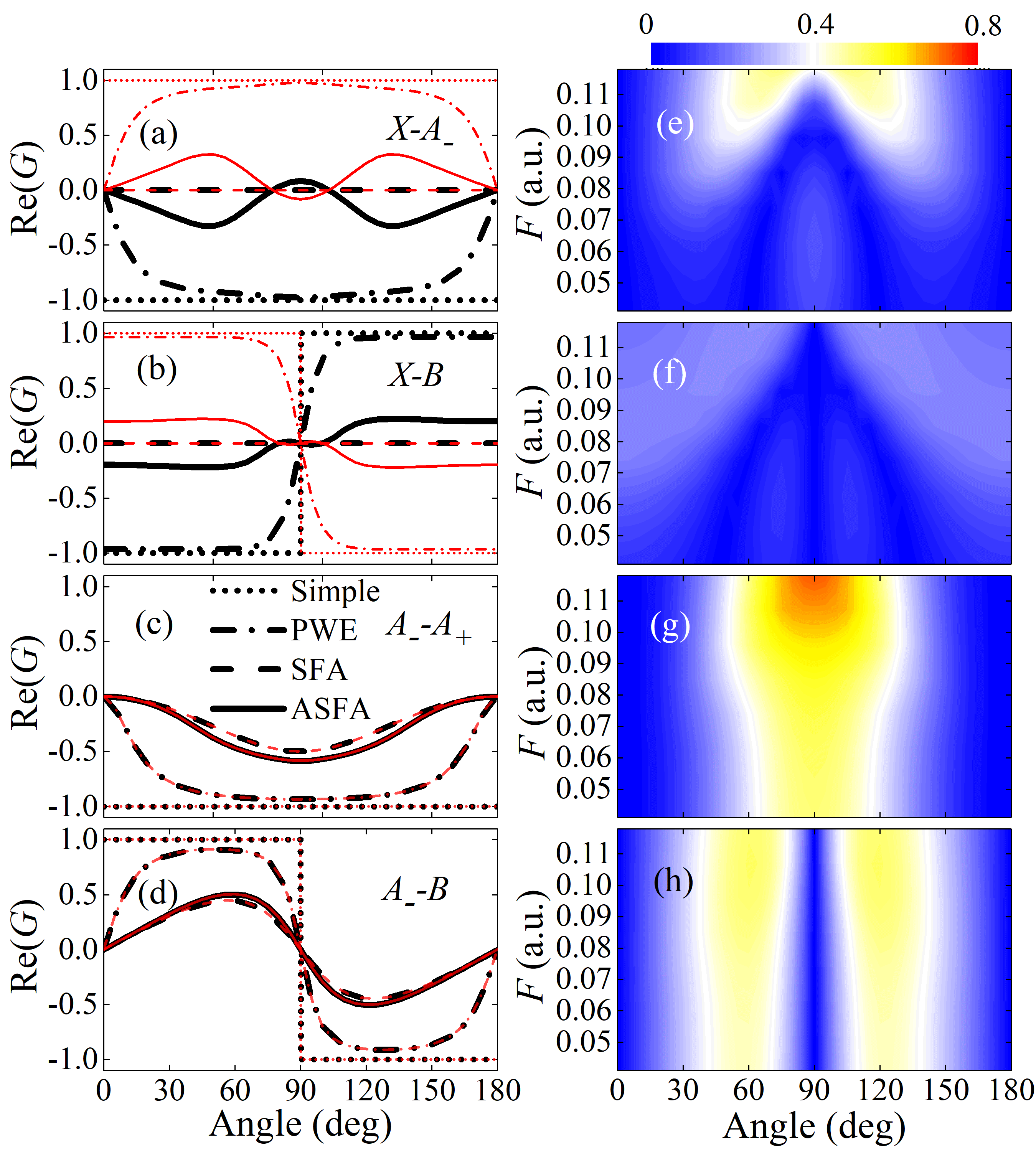
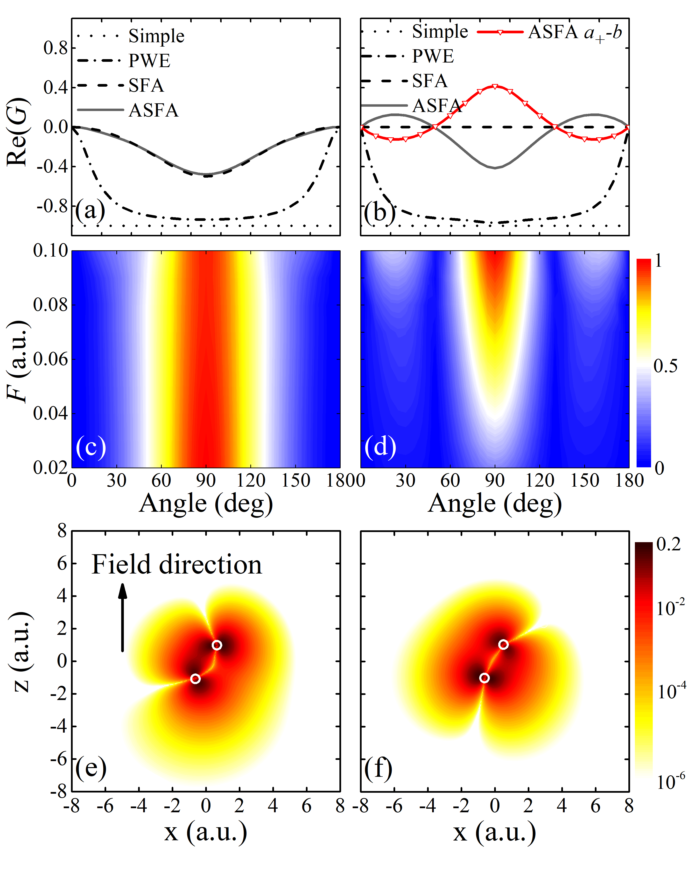
To investigate the effect of ionization-produced coherence on the dynamics of N, we first examine the properties of the coherence between ionic states produced at fixed electric field strengths. Figures 1(a)-1(d) show the complex DOC, , as a function of the angle between the molecular axis and the electric field, calculated using different coherence methods. Since only the PWE method gives the coherence with negligible imaginary parts, and the coherences calculated by other methods are purely real numbers (see Appendix), we display only the real parts of . Several features can be observed. (i) Except for the SFA method, all other methods predict the existence of the and coherences. (ii) Although the magnitudes of Re() obtained by different methods are different, their signs are the same except for the results of ASFA at the angle of . The structure of Re() around can be attributed to the counterintuitive shape of the distorted ionizing orbital (see Figs. 8(a) and 8(c) in the Appendix). Moreover, when the electric field is reversed, the following relationships are satisfied:
(iii) Quantitatively, the “Simple” method predicts the highest DOC of 100%, followed by the PWE method. In comparison, the ASFA and SFA methods predict lower DOCs . In the “Simple” method, we assume that the ionization primarily occurs in the opposite direction of the electric field. And the free-electron wavepackets ionized from different MOs are correlated with the same free-electron wavepacket. This means that the ionization amplitudes and are linearly dependent. As a result, the DOC between the ionic states is 100%, see Eq. 3. In the PWE method, ionization also occurs in the opposite direction of the electric field. But the partial ionization amplitudes and given by Eq. 7 are not linearly dependent. Therefore, the DOC is lower. In the ASFA and SFA methods, and are still not linearly dependent. Moreover, ionization occurs in all directions. More ionization directions result in a lower probability of the generated ionic states being correlated with the same free electron. After tracing out the free electrons, the DOC is significantly reduced.
We further discuss the dependence of ionization-produced coherence on the field strength. According to Eq. (4), the DOCs predicted by the “Simple” method do not rely on field strength. The same conclusion holds for the SFA method since the distortion of the ionizing MOs is not considered. For the PWE method, because the phase in Eq. (7) does not depend on the field strength, its predicted DOCs exhibit anomalous subtle decreases as the field strength increases (less than 5% within a.u.). Therefore, in Figs. 1(e)-1(h), we solely present the DOCs calculated by the ASFA method. As shown in Figs. 1(g) and 1(h), the DOCs between ionic states with the same parity ( and ) slightly decrease with the decreasing field strength, but do not disappear. This indicates that these DOCs are not sensitive to orbital distortion. However, for ionic states with opposite parity ( and ), the ionization-produced DOCs gradually emerge as the field strength increases, as shown in Figs. 1(e) and 1(f). Therefore, these DOCs are more dependent on the orbital distortion and more sensitive to the instantaneous field strength.
For the above results of and , we can provide the following explanation. At low field strengths, the orbital distortion is relatively small, and the parity of MOs can be well maintained. For ionizing MOs with opposite parity, the corresponding photoelectron wavepackets also carry opposite parity, and maintain orthogonality with one another. In this case, the generated ionic states cannot correlate with the same electronic continuum state, so there is no coherence between the two ionic states. Thus, the and DOCs approach zero at weak field strengths, as shown in Figs. 1(e) and 1(f). This implies that, within the multiphoton regime, the ionization-produced coherence primarily depends on the parities of the field-free MOs. On this condition, the SFA and ASFA methods give similar results. As the laser intensity increases, the parities of MOs will be disrupted due to the distortion of MOs. The electron wavepackets ionized from the distorted MOs are no longer orthogonal, so that different ionic states may correlate with the same electronic continuum state. Consequently, the coherence between the ionic states emerges after tracing out the free electrons. Therefore, in the tunnelling regime, the distortions of the ionizing MOs are crucial for the calculation of ionization-produced coherence, which is not captured in the standard SFA.
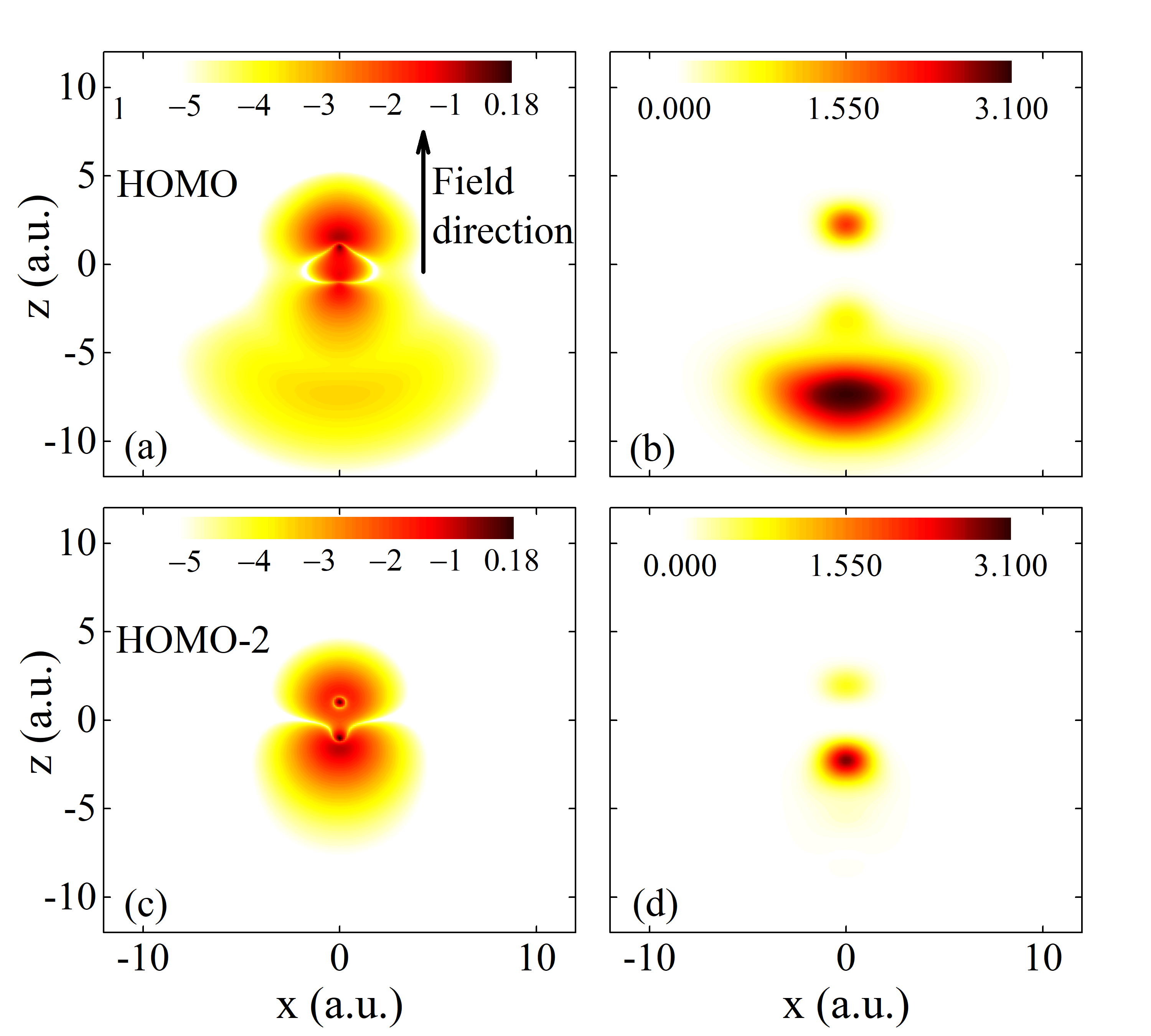
Fundamentally, only the free-field ground state is considered in the standard SFA. The lack of coupling with other states prevents MOs from exhibiting polarization effects under the influence of the electric field. In contrast, the ASFA method incorporates the polarization effect by considering orbital distortion. The orbital distortion causes the ionized free-electron wavepacket to exhibit pronounced directionality, thereby enhancing the coherence between the generated ionic states. To illustrate this point, we present the density distributions of the distorted orbitals and the ionized electrons in Fig. 2. The free-electron wavefunction ionized from the -th MO is calculated by . As shown in Figs. 2(a) and 2(c), the orbitals are stretched along the direction under the influence of the electric field. Consequently, these two distorted MOs tend to ionize along the direction, see Figs. 2(b) and 2(d). This increases the probability that the two ionic states are correlated with the same free electron. As a result, the coherence between the two ionic states is enhanced. However, the “Simple” and PWE methods adequately address, and even overestimate, the directionality of strong-field ionization. For instance, the PWE method considers only the ionization from the asymptotic regions of the orbital wavefunctions in the opposite direction of the electric field. Hence, these two methods are better suited for describing the coherence produced by tunnelling ionization, but they may overestimate the coherence generated at low laser intensities. In contrast, the ASFA method can be applied across a broader range of laser intensities due to its inclusion of field-dependent orbital distortion.
III.2 Post-ionization dynamics in N
Next, we focus on the influence of ionization-produced coherences on the dynamics of N. In the simulations, we use a linearly polarized 30-fs, 800-nm laser pulse with an intensity of W/cm2. Changing the wavelength will influence the effect of the ionization-produced coherence on the dynamics of N, as reflected in Eq. (21), which will be discussed later. Additionally, as discussed in our previous work Xue et al. (2021), the wavelength determines the pattern of the vibronic-state DOC after the pulse is over, with the maximum DOC occurring at . For ionizing orbitals with the same parities, is even; for those with opposite parities, is odd.
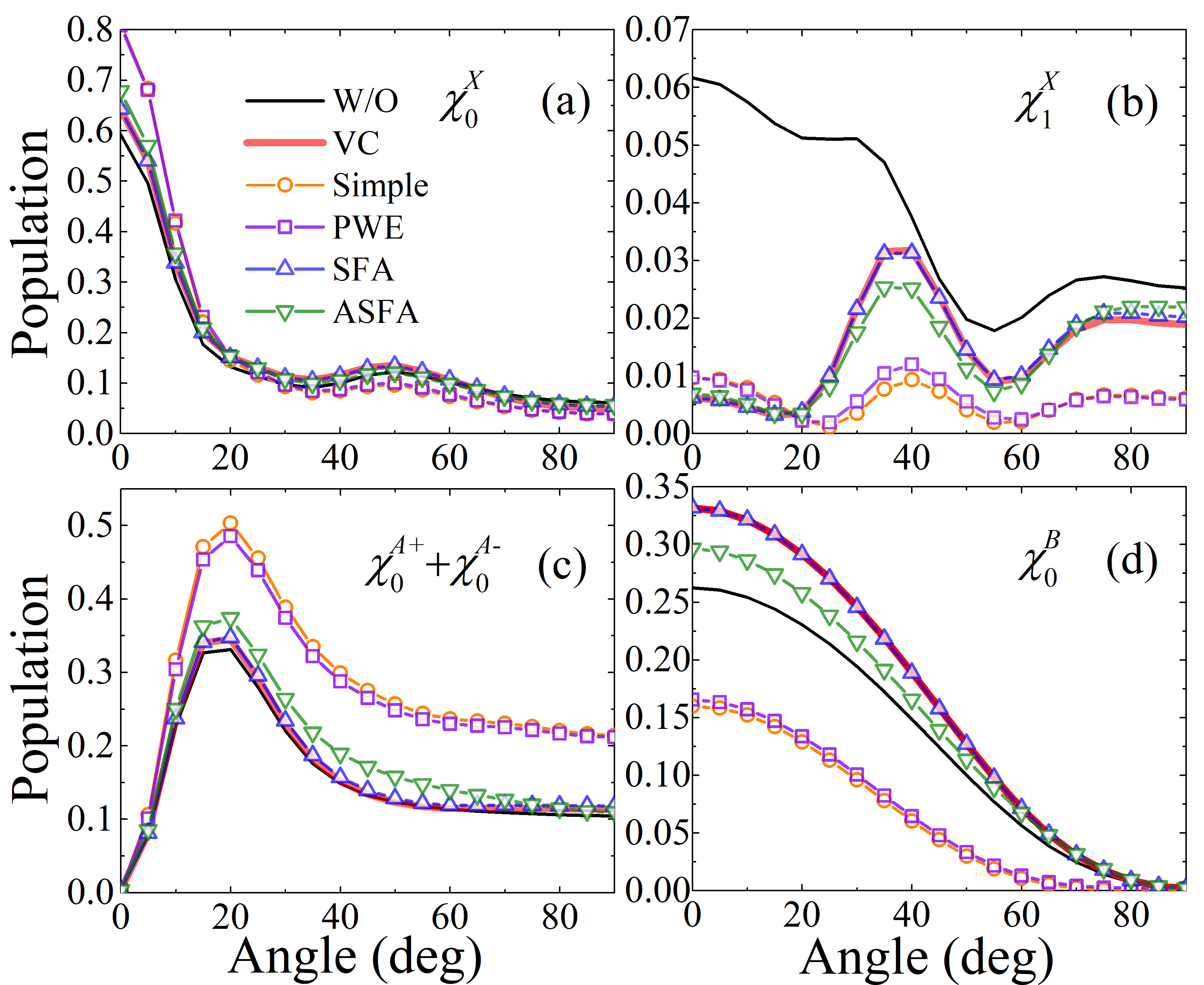
Figure 3 shows the populations of , , , and as functions of the molecular axis angle calculated under different conditions. These vibronic states are associated with N lasing at 391 nm and 428 nm Yao et al. (2011); Xu et al. (2015); Liu et al. (2015a, 2017); Britton et al. (2018); Kleine et al. (2022). By comparing the “VC” results with the “W/O” results, we find that the ionization-produced VCs cause a significant decrease in the population of , and an increase in the population of by up to . In contrast, the populations of and are almost unaffected by the VCs. To access the effect of ionization-produced VECs, we further compare the “Simple”, “PWE”, “SFA”, and “ASFA” results with the “VC” results. Several key features can be observed. (i) The “SFA” results overlap with the “VC” results. This is because the SFA predicts the absence of vibronic coherences for and (see Figs. 1(a) and 1(b)). (ii) Compared with the “VC” results, the populations calculated by the “Simple”, PWE, and ASFA methods undergo similar changes, although their magnitudes differ. For and , the ionization-produced VECs result in an increase in population at small angles. For and , the VECs induce population increases and decreases at nearly all angles, respectively. (iii) The “Simple” results exhibit the largest population changes, followed by the “PWE” results, while the “ASFA” results show relatively smaller changes. This finding is supported by the DOCs shown in Figs. 1(a-d), where the “Simple” method predicts the largest VECs, followed by the “PWE” results, and the ASFA method predicts smaller VECs.
To understand the effect of ionization-produced VCs on the transitions between ionic states, we employ a three-state (or V)-type model. States 1 and 3 are close in energy, mimicking two adjacent vibrational states of the same electronic state. State 2 mimics a vibronic state of a different electronic state. There are non-zero TDMs from states 1 and 3 to state 2. The quantum Liouville equations for this three-state system are as follows,
| (18) | ||||
If the instantaneous ionization-produced coherence is inserted at , the contribution of this term to should be
| (19) |
The sign of determines whether causes an increase or decrease in . This effect is due to the constructive or destructive interference between the pathways and . Using Eq. (19), we can explain the effect of the ionization-produced VCs. Taking the transition as an example, we analyze the transition process. For the electronic state, the most populated vibrational states are and . Therefore, the transition is dominated by the pathways and . Specifically, states , , and correspond to states 1, 2, and 3 in the three-state model, respectively. And corresponds to . Given that , and , the two pathways interfere constructively. Therefore, when incorporating the ionization-produced VCs, increases appreciably, while decreases significantly. The population changes of other vibronic states can also be analyzed in a similar manner.
To understand the effect of the ionization-produced VECs, we adopt a two-state model interacting with an electric field . Under the rotating wave approximation, the two-state DM equations can be written as
| (20) | ||||
where , and . represents the instantaneous ionization-produced VEC. Because , the population transfer caused by can be assessed by
| (21) |
In the derivation, we consider that the imaginary part of the VEC is negligible (see Appendix). According to this equation, the population transfer caused by depends on , the frequency detuning and the integral term. For the molecular axis angles smaller than , has a sign opposite to the electric field (see Fig. 1), resulting in a negative integration term. Taking and transitions as examples, , , so is negative. This means that the ionization-produced VEC has a suppressive effect on the transition from (or ) to . Therefore, compared to the “VC” results, and are increased, while is decreased in the “Simple”, “PWE”, and “ASFA” results (see Figs. 3(a), 3(b), and 3(d)). For the transition, since , the detuning can be either positive or negative. As a result, the ionization-produced VEC can either promote or suppress the transitions. Specifically, for the transition, . Namely, the VEC enhances the transition, thereby resulting in the increase of the (see Fig. 3(c)). Furthermore, according to Eq. (21), we also find that the laser wavelength can be utilized to manipulate the ionization-produced VECs by adjusting the detuning between the vibronic-state energy difference and the laser frequency, thereby controlling the post-ionization molecular dynamics of the residual ions.
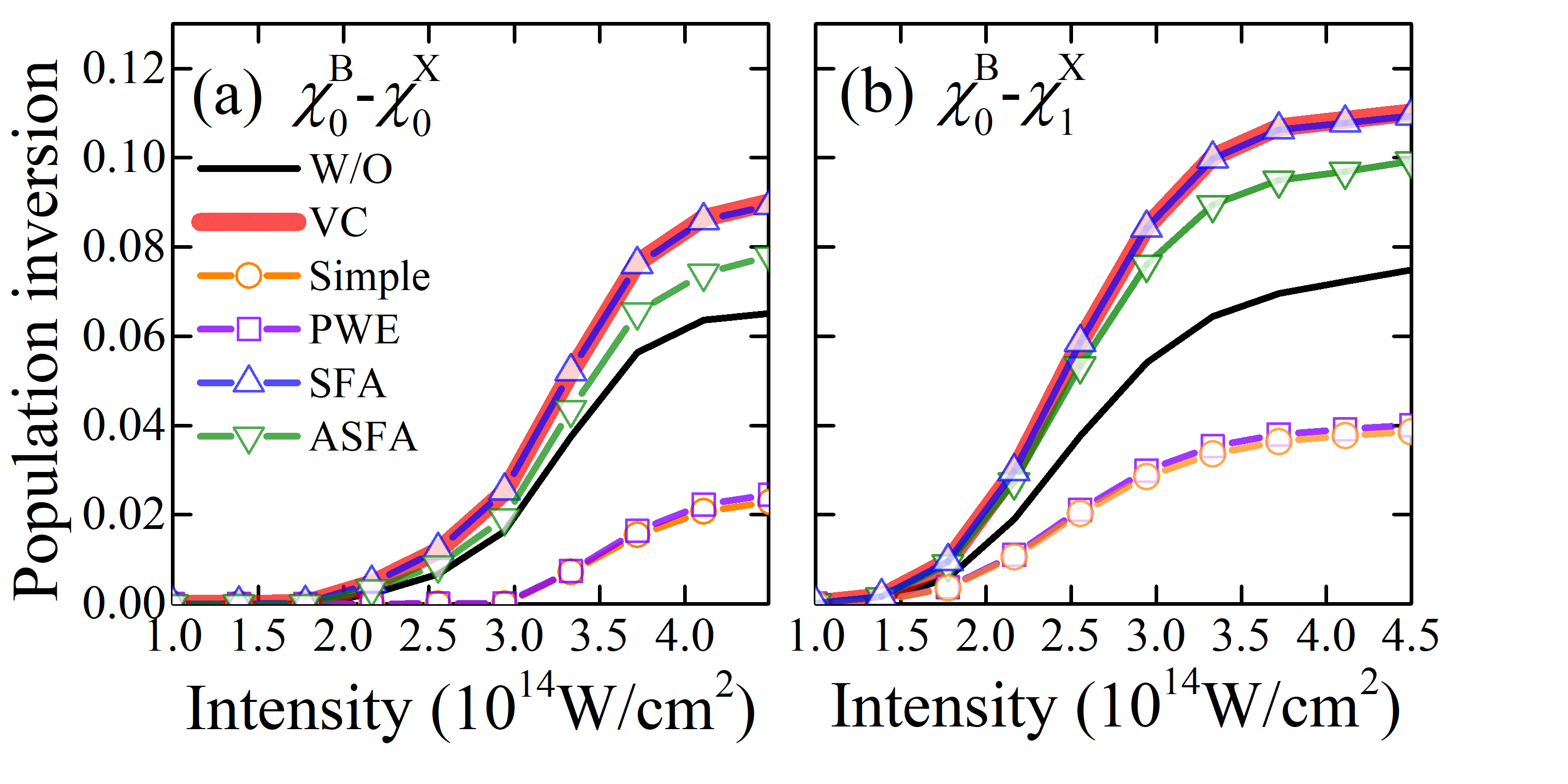
Compared to the populations of individual states, we are more interested in the population inversion between and , as it directly relates to the N lasing generation in ambient air Yao et al. (2011); Xu et al. (2015); Liu et al. (2015a, 2017); Britton et al. (2018); Kleine et al. (2022). Figures 4(a) and 4(b) respectively show the population inversions between and , and between and as functions of laser intensity. The results are obtained by integrating the signals over molecular axis angles where the population inversion is positive. Obviously, the population inversions in both cases are strongly enhanced when considering the ionization-produced VCs. In contrast, when the ionization-produced VECs are incorporated, the population inversions are suppressed compared to the VC results, as shown in the “Simple”, “PWE”, and “ASFA” results. Because the VECs of and predicted by the SFA method are zero, the “SFA” and “VC” results nearly overlap. Overall, the “Simple” and “PWE” results are similar, showing reductions of over 50% compared to the “W/O” results. This increases the laser intensity threshold for the - population inversion to approximately W/cm2. However, as shown in Fig. 4(a), the laser intensity threshold predicted by the ASFA method is around W/cm2, which is consistent with the experimental finding for the 391-nm lasing in Ref. Liu et al. (2015b). Moreover, although the results of ASFA are slightly lower than those of the “VC”, ionization-produced coherences still enhance the population inversion of by up to 20% and that of by up to 30%.
III.3 Ionization-produced coherence in O
We now investigate the post-ionization dynamics of O2, focusing on the influence of the ionization-produced coherence on the dissociation signals of O. When a strong laser field interacts with O2, electrons can be ionized from the HOMO (1), HOMO-1 (1), and HOMO-2 (3) orbitals, resulting in the formation of O in the X, and electronic states, respectively. on the subscript denotes the orbital angular momentum along the molecular axis, with values of . Subsequently, O can dissociate along the potential curve by the transition De et al. (2011); Magrakvelidze et al. (2012); Cörlin et al. (2015). Our previous studies verified that the state also plays a crucial role in the dissociation process through a pathway of when the and states are resonantly coupled by the laser field Xue et al. (2018). However, the state is not coupled to the other three states because of its distinct spin multiplicity, and is therefore excluded from the simulations. Consequently, only the states a, and f are included in the simulations, and denoted as , , and for simplicity. As known, the TDMs are parallel to the molecular axis, while the TDMs are perpendicular to the molecular axis Xue et al. (2018).
First, we discuss the properties of the ionization-produced coherence. Figures 5(a) and 5(b) show the ionization-produced complex DOC as a function of molecular axis angle at a fixed field strength of =0.09 a.u. Similar to Fig. 1, only the real parts of are displayed. Three features can be observed. (i) The coherence between and calculated by the SFA method is zero, as shown in Fig. 5(b). This is because the parities of the field-free ionizing orbitals and are opposite, making the corresponding electronic continuum states orthogonal. As a result, there is no coherence between states and . (ii) Similar to N, the “Simple” method predicts the highest DOC , followed by the PWE method, while the SFA and ASFA methods predict lower DOCs . This feature can be understood as follows. In comparison with the “Simple” and PWE methods, which primarily consider ionizations occurring in the opposite direction of the field, the SFA (or ASFA) method considers ionizations in all directions. More ionization directions result in a lower probability that the generated ionic states are correlated with the same free electron. Consequently, the DOC between the ionic states reduces. (iii) Although the values of Re predicted by different methods differ, their signs are the same, except for Re calculated by the ASFA method around and . This exception can be attributed to the counterintuitive shape of the orbital at these angles, from which ionization produces the ionic state . More specifically, in our DFT calculations, the configuration of the ground state X in O2 is , where the two unpaired electrons both have spin. Therefore, the -spin orbital should be ionized to produce the spin quartet ionic states . Taking the orbital as an example, we show the electron densities of the distorted orbitals with spin and at in Figs. 5(e) and 5(f), respectively. It can be seen that the -spin orbital tends to stretch in the opposite direction of the applied field. However, the -spin orbital does not stretch in the opposite direction of the electric field. This is because the -spin orbital is influenced not only by the field but also by the Coulomb repulsion from the -spin orbital. This counterintuitive shape of the -spin orbital ultimately leads to the abnormal sign of the coherence around .
We further discuss the effect of field strength on the DOC. Since the DOCs predicted by the “Simple”, PWE, and SFA methods remain constant or nearly unchanged with varying field strength, we present only the ASFA results in Figs. 5(c) and 5(d). As shown, the DOC hardly changes with field strength. In contrast, the DOC gradually increases with increasing field strength. This indicates that the DOC is not sensitive to orbital distortion, whereas the DOC is. This difference can be understood as follows. The ionic states and are generated by the ionization of MOs and . The two MOs possess the same parity. When not considering orbital distortion, the free-electron wavepackets generated from these two MOs also have the same parity. Consequently, after tracing out the states of the free electron, there is always coherence between states and . In contrast, the ionic state comes from the ionization of the orbital, which has the opposite parity to the orbitals. When not considering orbital distortion, the electrons ionized from the and orbitals can not occupy the same quantum state. Therefore, there is no coherence between states and in the case. Because the ASFA method considers the effect of orbital distortion, the electrons ionized from the distorted and orbitals can have a nonzero probability of occupying the same quantum state. As a result, the coherence emerges. Moreover, the stronger the field strength, the more severe the orbital distortion. Therefore, the coherence between states and increases with increasing field strength.
III.4 Post-ionization dynamics in O
In the following, we explore the role of ionization-produced coherences in the dissociative ionization dynamics of O2. In the simulations, a linearly polarized 800-nm, 30-fs laser pulse with an intensity of is used. At this wavelength, the electronic states and are resonantly coupled. Figure 6(a) shows the dissociation probabilities as a function of the molecular axis angle , calculated under different conditions. By comparing the “VC” results with the “W/O” results, it is found that the VC enhances the dissociation probability at small angles while reducing it at large angles. This can be explained as follows. At small angles, the parallel transition dominates. Based on Eq. (19), the ionization-produced VCs in the state will increase the transitions, leading to an enhancement of the dissociation probability. As the angle increases, the perpendicular transitions gradually become strong. The VCs increase the transition of this pathway, thereby reducing the population of the state. As a result, the dissociation probability is weakened. Next, we discuss the effect of the ionization-produced VECs. As shown, compared to the “VC” results, the “Simple”, PWE, SFA, and ASFA methods predict weaker dissociation signals. This is because the ionization-produced coherence enhances the transition, thereby weakening the dissociative process. The enhancement of the transition can be interpreted within the frame of the -type three-state model. Specifically, states and correspond to states 1 and 3 in Eq. (19), respectively. It can be seen from Fig. 5(a) that the coherence is smaller than zero. Moreover, the interacting term satisfies , which holds for all molecular axis angles and field directions. Consequently, the and transitions interfere constructively, leading to an overall enhancement of the transitions. In addition, since the SFA and ASFA methods predict comparable coherence (see Fig. 6(c)), their predicted dissociation probabilities are nearly identical. However, the “Simple” and PWE methods predict higher coherences, so they predict much weaker dissociation signals.
The influence of the ionization-produced coherences is also reflected in the KER spectrum. Figure 6(b) shows the KER spectra calculated at . This angle is chosen because ion signals were collected along the direction perpendicular to the laser polarization in previous experiments Zohrabi et al. (2011); De et al. (2011). Compared with the “W/O” result, the intensity of the “VC” spectrum reduces. After introducing the ionization-produced VEC, the “ASFA” signals show an additional 40% decrease. Moreover, both the “VC” and “ASFA” spectra exhibit peak structures, as observed in the single-pulse and the IR-pump-IR-probe experiments Zohrabi et al. (2011); De et al. (2011). The peaks are primarily induced by the ionization-produced VC and correspond to the projection of vibrational states onto the dissociative continuum states Xue et al. (2018). These significant changes suggest the importance of the ionization-produced VCs and VECs in simulating the dissociative ionization dynamics of O2.
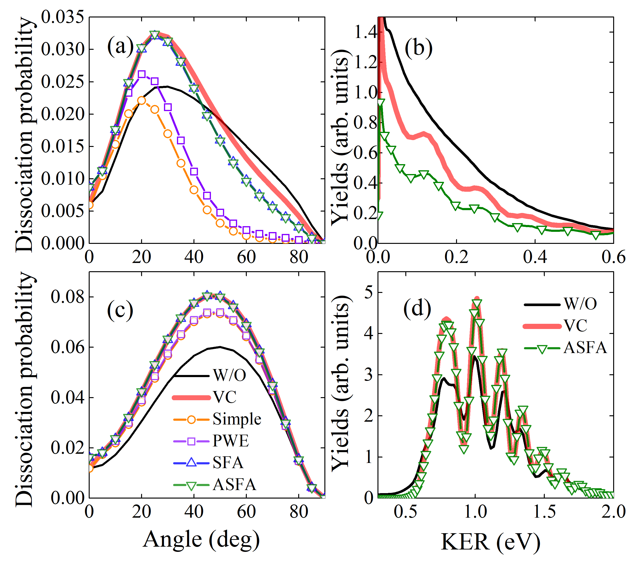
To further assess the role of the ionization-produced VECs, we change the laser wavelength to 400 nm. In this case, the resonant transitions between states and state are almost closed. Figure 6(c) presents the corresponding angle-dependent dissociation probabilities. One can see that only the ionization-produced VCs increase the dissociation signal at nearly all angles by enhancing the transitions. However, the influence of the ionization-produced VECs remains notably weak, even for the “Simple” and PWE methods, where the VECs are expected to be stronger (see Figs. 5(a) and 5(b)). Figure 6(d) shows the corresponding KER spectra at . The spectra calculated under the “VC” condition and by the ASFA method almost overlap and are stronger than the “W/O” result. This indicates that the ionization-produced VECs play a negligible role when the electronic states are not strongly coupled.
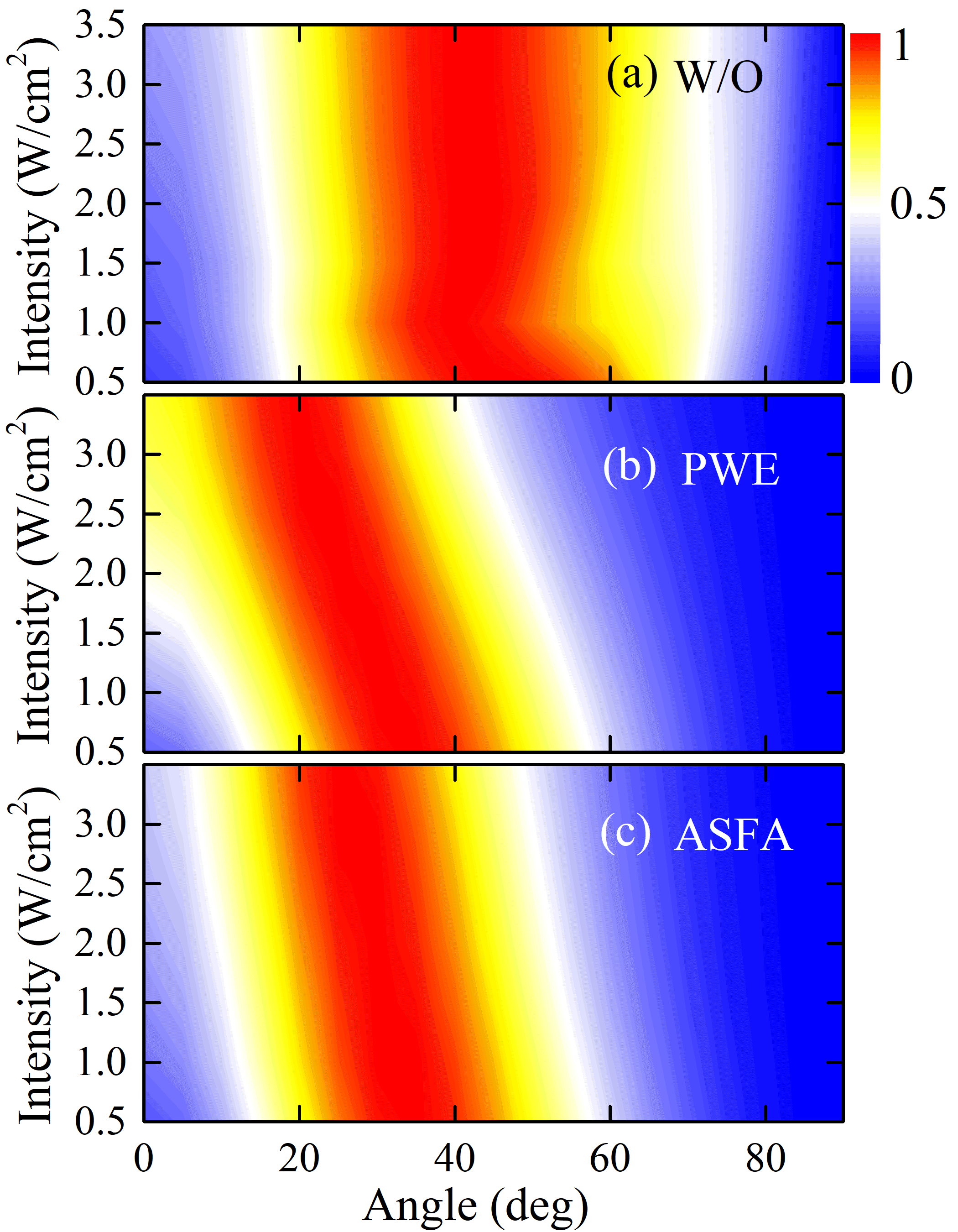
Finally, in order to detect the signatures of the ionization-produced coherences in O, we suggest performing a laser intensity scan on the angular-dependent dissociation signals. Figure 7 presents the corresponding results of different methods. An 800-nm 10-fs laser pulse is used here, which can lead to the resonant transition. We focus on the angle with the maximum dissociation signal, which is denoted as the peak angle. As shown, different methods give different slopes for the peak angle as a function of laser intensity. This phenomenon can be understood by considering the competition between the parallel transition and the perpendicular transition. Recalling that the ionization-induced coherence enhances the transition, we note two key factors. First, according to Eq. (19), the enhancement becomes more pronounced with increasing field strength. Second, the DOC increases as the molecular axis angle changes from to (see Fig. 5(c)), meaning that the enhancement becomes stronger as the angle approaches . These two factors lead to a reduced population of the state at larger angles with increasing laser intensity, resulting in less dissociation through the pathway. Consequently, the peak angle shifts to a smaller angle with increasing laser intensity. In the PWE method, the coherence is strong (see Fig. 5(a)), so the signal peak shifts toward smaller angles as the laser intensity increases, as shown in Fig. 7(b). In the ASFA method, the coherence is relatively weak, so the peak angle changes less, as shown in Fig. 7(c). Under the “W/O” condition, the ionization-produced coherence is not considered, so the peak angle remains almost unchanged, as shown in Fig. 7(a). By calibrating the slope of the peak angle, the signatures of the ionization-produced coherence can be detected.
IV CONCLUSION
In summary, we present an ASFA method to predict the ionic coherence generated by multi-orbital strong-field ionizations. Due to consideration of orbital distortion, the ASFA method overcomes the limitations of the standard SFA, and enables ionic states of different parities to correlate with the same electronic continuum state, resulting in the generation of coherence between these states in the residual ions. Moreover, we find that both the “Simple” and PWE methods are more applicable in the tunnelling regime due to the assumption that ionization primarily occurs in the opposite direction of the electric field. In contrast, the ASFA method can provide reasonable ionization-produced coherence within a broader range of laser intensities.
Besides, we also examine the effect of ionization-produced coherences on the transitions between electronic states in the residual ions. For N, the VCs enhance the population inversion, whereas the VECs reduce it. Overall, the ASFA method predicts that ionization-produced coherences increase the population inversion by approximately 25%30%. As a result, the laser intensity threshold for achieving this inversion is reduced, making it more consistent with the experimental value. For O, the coherences enhance both the and transitions. The competition between the two pathways weakens the dissociation via the transition. By choosing a 400-nm wavelength that nearly closes the transition, we found that the ionization-produced coherences can enhance the dissociation probability by more than 30%. These results highlight the importance of ionization-produced coherences in post-ionization molecular dynamics. Accurately manipulating these coherences can offer a promising avenue for controlling post-ionization molecular dynamics and should attract more attention from the strong-field community.
ACKNOWLEDGEMENT
This work was supported by the National Natural Science Foundation of China (Grants No. 12274188, No. 12004147, No. 12204209), the Natural Science Foundation of Gansu Province (Grant No. 23JRRA1090), and the Fundamental Research Funds for the Central Universities (Grant No. lzujbky-2023-ey08).
APPENDIX: analysis of the coherence phase upon strong-field ionization
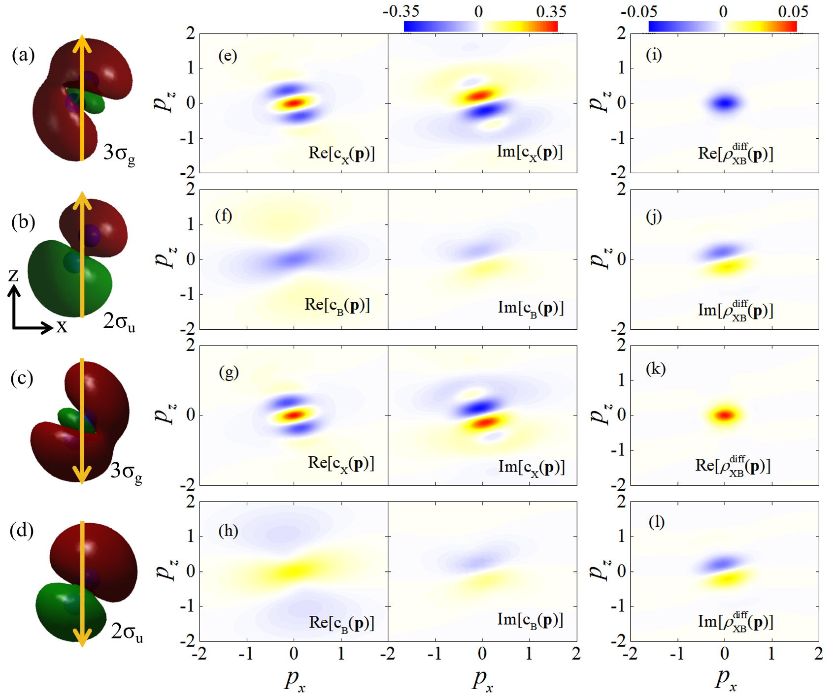
Here, we analyze the phase of the ionization-produced coherence calculated by the ASFA coherence method. In this method, according to Eq. (13), the instantaneously produced coherence depends on , where , with representing the wavefunction of the ionizing MO. Due to field-induced distortion, the parity of is destroyed, so that is neither purely real nor purely imaginary. As a result, is theoretically expected to be a complex number. However, numerical calculations indicate that is still real, which is not easy to understand intuitively. Therefore, a detailed analysis is provided below.
To illustrate this issue, we take the ionization-produced coherence in N as an example. Figures 8(a)-8(d) display the distorted HOMO () and HOMO-2 () orbitals at external field strengths of a.u. The angle between the molecular axis and the laser polarization (-axis) is set to . Figures 8(e)-8(h) show the corresponding ionization amplitude . Here, is the electric field along the space axis. For simplicity, is restricted to the plane. It can be seen that Re is symmetric with respect to the inversion of , while Im is antisymmetric. We define as the ionization-produced differential coherence. Real and imaginary parts of are presented in Figs. 8(i) and 8(j) for a.u., and in Figs. 8(k) and 8(l) for a.u. As shown, the real part of is also symmetric with respect to the inversion of , while the imaginary part is antisymmetric. Recalling that , the imaginary part cancels out upon integration over due to the symmetry properties of . Therefore, is real.
Additionally, we also find that the real parts of are negative for and positive for . This behavior can be attributed to the symmetric relation between the MOs produced by the positive and negative fields, i.e.,
Therefore,
These relations are clearly illustrated in Figs. 8(a-h). Finally, one can obtain . As a result, the real part of the coherence changes sign when the field reverses.
Besides, it is noteworthy that the orbital exhibits a counterintuitive distortion. Namely, a portion of the red part of the orbital twists along the field direction. This effect becomes more pronounced as approaches 90∘. This anomalous distortion, likely arising from multi-orbital interactions in the self-consistent field calculation, is closely related to the structure between 60∘ and 120∘ in the ASFA’s results, as shown in Fig. 1(a).
References
- McFarland et al. (2008) B. K. McFarland, J. P. Farrell, P. H. Bucksbaum, and M. Gühr, Science 322, 1232 (2008).
- Smirnova et al. (2009) O. Smirnova, Y. Mairesse, S. Patchkovskii, N. Dudovich, D. Villeneuve, P. Corkum, and M. Y. Ivanov, Nature 460, 972 (2009).
- Pabst et al. (2016) S. Pabst, M. Lein, and H. J. Wörner, Phys. Rev. A 93, 023412 (2016).
- Goulielmakis et al. (2010) E. Goulielmakis, Z. Loh, A. Wirth, R. Santra, N. Rohringer, V. S. Yakovlev, S. Zherebtsov, T. Pfeifer, A. M. Azzeer, M. F. Kling, S. R. Leone, and F. Krausz, Nature 466, 739 (2010).
- Wirth et al. (2011) A. Wirth, M. T. Hassan, I. Grguraš, J. Gagnon, A. Moulet, T. T. Luu, S. Pabst, R. Santra, Z. A. Alahmed, A. M. Azzeer, V. S. Yakovlev, V. Pervak, F. Krausz, and E. Goulielmakis, Science 334, 195 (2011).
- Kraus et al. (2013) P. M. Kraus, S. B. Zhang, A. Gijsbertsen, R. R. Lucchese, N. Rohringer, and H. J. Wörner, Phys. Rev. Lett. 111, 243005 (2013).
- Calegari et al. (2014) F. Calegari, D. Ayuso, A. Trabattoni, L. Belshaw, S. De Camillis, S. Anumula, F. Frassetto, L. Poletto, A. Palacios, P. Decleva, J. B. Greenwood, F. Martín, and M. Nisoli, Science 346, 336 (2014).
- Breidbach and Cederbaum (2003) J. Breidbach and L. S. Cederbaum, J. Chem. Phys. 118, 3983 (2003).
- Breidbach and Cederbaum (2005) J. Breidbach and L. S. Cederbaum, Phys. Rev. Lett. 94, 033901 (2005).
- Belshaw et al. (2012) L. Belshaw, F. Calegari, M. J. Duffy, A. Trabattoni, L. Poletto, M. Nisoli, and J. B. Greenwood, J. Phys. Chem. Lett. 3, 3751 (2012).
- Hennig et al. (2005) H. Hennig, J. Breidbach, and L. S. Cederbaum, J. Phys. Chem. A 109, 409 (2005).
- Wörner et al. (2017) H. J. Wörner, C. A. Arrell, N. Banerji, A. Cannizzo, M. Chergui, A. K. Das, P. Hamm, U. Keller, P. M. Kraus, E. Liberatore, P. Lopez-Tarifa, M. Lucchini, M. Meuwly, C. Milne, J. E. Moser, U. Rothlisberger, G. Smolentsev, J. Teuscher, J. A. van Bokhoven, and O. Wenger, Struct. Dynam. 4, 061508 (2017).
- Palacios et al. (2006) A. Palacios, H. Bachau, and F. Martín, Phys. Rev. Lett. 96, 143001 (2006).
- Ishikawa and Sato (2015) K. L. Ishikawa and T. Sato, IEEE J. Sel. Top. Quant. 21, 1 (2015).
- Vacher et al. (2017) M. Vacher, M. J. Bearpark, M. A. Robb, and J. P. Malhado, Phys. Rev. Lett. 118, 083001 (2017).
- Chen et al. (2019) J. Chen, J. Yao, H. Zhang, Z. Liu, B. Xu, W. Chu, L. Qiao, Z. Wang, J. Fatome, O. Faucher, C. Wu, and Y. Cheng, Phys. Rev. A 100, 031402 (2019).
- Zhang et al. (2020) Q. Zhang, H. Xie, G. Li, X. Wang, H. Lei, J. Zhao, Z. Chen, J. Yao, Y. Cheng, and Z. Zhao, Commun. Phys. 3, 50 (2020).
- Lei et al. (2022) H. Lei, J. Yao, J. Zhao, H. Xie, F. Zhang, H. Zhang, N. Zhang, G. Li, Q. Zhang, X. Wang, et al., Nat. Commun. 13, 4080 (2022).
- Yuen and Lin (2022) C. H. Yuen and C. D. Lin, Phys. Rev. A 106, 023120 (2022).
- Yuen et al. (2023) C. H. Yuen, P. Modak, Y. Song, S.-F. Zhao, and C. D. Lin, Phys. Rev. A 107, 013112 (2023).
- Rohringer and Santra (2009) N. Rohringer and R. Santra, Phys. Rev. A 79, 053402 (2009).
- Carlström et al. (2017) S. Carlström, J. Mauritsson, K. J. Schafer, A. L’Huillier, and M. Gisselbrecht, J. Phys. B: At. Mol. Opt. 51, 015201 (2017).
- Vacher et al. (2015) M. Vacher, L. Steinberg, A. J. Jenkins, M. J. Bearpark, and M. A. Robb, Phys. Rev. A 92, 040502 (2015).
- Arnold et al. (2017) C. Arnold, O. Vendrell, and R. Santra, Phys. Rev. A 95, 033425 (2017).
- Xue et al. (2021) S. Xue, S. Yue, H. Du, B. Hu, and A.-T. Le, Phys. Rev. A 104, 013101 (2021).
- Zhu et al. (2023) Z. Zhu, S. Xue, Y. Zhang, Y. Zhang, R. Yang, S. Sun, Z. Liu, P. Ding, and B. Hu, Phys. Rev. A 108, 013111 (2023).
- Yuen and Lin (2023) C. H. Yuen and C. D. Lin, Phys. Rev. A 108, 023123 (2023).
- Tolstikhin et al. (2011) O. I. Tolstikhin, T. Morishita, and L. B. Madsen, Phys. Rev. A 84, 053423 (2011).
- Tong et al. (2002) X.-M. Tong, Z. X. Zhao, and C.-D. Lin, Phys. Rev. A 66, 033402 (2002).
- Zhao et al. (2010) S.-F. Zhao, C. Jin, A.-T. Le, T. F. Jiang, and C. D. Lin, Phys. Rev. A 81, 033423 (2010).
- Śpiewanowski et al. (2013) M. D. Śpiewanowski, A. Etches, and L. B. Madsen, Phys. Rev. A 87, 043424 (2013).
- Śpiewanowski and Madsen (2014) M. D. Śpiewanowski and L. B. Madsen, Phys. Rev. A 89, 043407 (2014).
- Śpiewanowski and Madsen (2015) M. D. Śpiewanowski and L. B. Madsen, Phys. Rev. A 91, 043406 (2015).
- Song et al. (2023) S. Song, M. Zhu, H. Ni, and J. Wu, Comput. Phys. Commun. 292, 108882 (2023).
- (35) M. J. Frisch, G. W. Trucks, and H. B. S. et al., Gaussian˜16 Revision C.01, Gaussian Inc. Wallingford CT (2016).
- Yao et al. (2011) J. Yao, B. Zeng, H. Xu, G. Li, W. Chu, J. Ni, H. Zhang, S. L. Chin, Y. Cheng, and Z. Xu, Phys. Rev. A 84, 051802 (2011).
- Xu et al. (2015) H. Xu, E. Lötstedt, A. Iwasaki, and K. Yamanouchi, Nat. Commun. 6, 8347 (2015).
- Liu et al. (2015a) Y. Liu, P. Ding, G. Lambert, A. Houard, V. Tikhonchuk, and A. Mysyrowicz, Phys. Rev. Lett. 115, 133203 (2015a).
- Liu et al. (2017) Y. Liu, P. Ding, N. Ibrakovic, S. Bengtsson, S. Chen, R. Danylo, E. R. Simpson, E. W. Larsen, X. Zhang, Z. Fan, A. Houard, J. Mauritsson, A. L’Huillier, C. L. Arnold, S. Zhuang, V. Tikhonchuk, and A. Mysyrowicz, Phys. Rev. Lett. 119, 203205 (2017).
- Britton et al. (2018) M. Britton, P. Laferrière, D. H. Ko, Z. Li, F. Kong, G. Brown, A. Naumov, C. Zhang, L. Arissian, and P. B. Corkum, Phys. Rev. Lett. 120, 133208 (2018).
- Kleine et al. (2022) C. Kleine, M.-O. Winghart, Z.-Y. Zhang, M. Richter, M. Ekimova, S. Eckert, M. J. J. Vrakking, E. T. J. Nibbering, A. Rouzée, and E. R. Grant, Phys. Rev. Lett. 129, 123002 (2022).
- Liu et al. (2015b) Y. Liu, P. Ding, G. Lambert, A. Houard, V. Tikhonchuk, and A. Mysyrowicz, Physical Review Letters 115, 133203 (2015b).
- De et al. (2011) S. De, M. Magrakvelidze, I. A. Bocharova, D. Ray, W. Cao, I. Znakovskaya, H. Li, Z. Wang, G. Laurent, U. Thumm, M. F. Kling, I. V. Litvinyuk, I. Ben-Itzhak, and C. L. Cocke, Phys. Rev. A 84, 043410 (2011).
- Magrakvelidze et al. (2012) M. Magrakvelidze, C. M. Aikens, and U. Thumm, Phys. Rev. A 86, 023402 (2012).
- Cörlin et al. (2015) P. Cörlin, A. Fischer, M. Schönwald, A. Sperl, T. Mizuno, U. Thumm, T. Pfeifer, and R. Moshammer, Phys. Rev. A 91, 043415 (2015).
- Xue et al. (2018) S. Xue, H. Du, B. Hu, C. D. Lin, and A.-T. Le, Phys. Rev. A 97, 043409 (2018).
- Zohrabi et al. (2011) M. Zohrabi, J. McKenna, B. Gaire, N. G. Johnson, K. D. Carnes, S. De, I. A. Bocharova, M. Magrakvelidze, D. Ray, I. V. Litvinyuk, C. L. Cocke, and I. Ben-Itzhak, Phys. Rev. A 83, 053405 (2011).