Coherent Solutions and Transition to Turbulence in Two-Dimensional Rayleigh-Bénard Convection
Abstract
For two-dimensional (2D) Rayleigh-Bénard convection, classes of unstable, steady solutions were previously computed using numerical continuation [1, 2]. The ‘primary’ steady solution bifurcates from the conduction state at , and has a characteristic aspect ratio (length/height) of approximately . The primary solution corresponds to one pair of counterclockwise-clockwise convection rolls with a temperature updraft in between and an adjacent downdraft on the sides. By adjusting the horizontal length of the domain, [1, 2] also found steady, maximal heat transport solutions, with characteristic aspect ratio less than and decreasing with increasing . Compared to the primary solutions, optimal heat transport solutions have modifications to boundary layer thickness, the horizontal length scale of the plume, and the structure of the downdrafts. The current study establishes a direct link between these (unstable) steady solutions and transition to turbulence for and . For transitional values of , the primary and optimal-heat-transport solutions both appear prominently in appropriately-sized sub-fields of the time-evolving temperature fields. For beyond transitional, our data analysis shows persistence of the primary solution for , while the optimal heat transport solutions are more easily detectable for . In both cases and , the relative prevalence of primary and optimal solutions is consistent with the vs. scalings for the numerical data and the steady solutions.
I Introduction
Thermal convection is heat transfer in liquids and gases resulting from buoyancy-driven fluid motion, and is fundamental for establishing circulations in the earth’s atmosphere and oceans, planetary mantle dynamics, stellar evolution, as well as a broad range of engineering applications [3]. Rayleigh-Bénard convection (RBC) refers to convection generated by simplified dynamical equations and idealized boundary conditions. The simplified equations are called the Oberbeck-Boussinesq approximation, describing viscous fluids that are mechanically incompressible but thermally expansible [see, e.g., 4, and references therein]. The domain is confined between two parallel plates, heated from below and cooled from above such that the bottom plate is always warmer than the top plate by a fixed temperature difference. The Rayleigh-Bénard setup presents a framework that is at the same time experimentally realizable, analytically tractable and numerically accessible [see 5, 6, for overviews]. Its prominence in the literature stems partly from its practical importance, and partly from the fact that Rayleigh-Bénard convection represents a rich nonlinear dynamics to test physical reasoning and mathematical techniques.
In the Rayleigh-Bénard convection problem, the Rayleigh number and the Prandtl number are nondimensional parameters that control the flow dynamics: characterizes the relative strength of buoyancy-driven inertial forces to viscous forces and is the ratio of the kinematic viscosity to the thermal diffusivity. Furthermore, a key nondimensional diagnostic parameter is the Nusselt number , measuring the vertical heat transport for a given temperature difference between the plates. Over the last several decades, there has been an intense focus on the scaling behavior of on and . This relationship has been explored via experiments [7, 8, 9, 5, 10, 11, 12], scaling laws [13, 14, 15, 16, 17, 18, 19, 20], rigorous upper bounds on the allowable heat transport [21, 22, 23, 24, 25], and numerical simulations [26, 27, 1, 2, 28, 29, 30, 31, 32, 33]. The two competing scaling behaviors that emerge from this body of work are and . The scaling, often referred to as the classical scaling, emerges from physical arguments [13, 14] involving independence of top and bottom boundary layers [14] as well as marginal stability of the boundary layers [13, 17]. The scaling, recently referred to as the ultimate regime, emanates from mixing length theories of turbulence [16, 15]. There has been a flurry of recent activity on the possible transition from scaling to scaling , e.g. experiments by [7, 34, 11, 12]. Several studies have also been aimed at accessing the regime for , and at verifying (or not) the existence of the scaling [35, 12, 36, 37, 38, 39, 40, 30]. Such considerations are beyond the scope of our work in this paper. We note that the flow Reynolds number can be expressed in terms of and , and that the precise relationship is also of interest to researchers [19, 41, 42]. Interestingly, rigorous upper bounds on heat transport are sensitive to the boundary conditions, being bounded by in the no-slip case [23] and by in the 2D free-slip case [43, 44]. We also mention that substantial effort has been devoted to determining the effect of on the heat transport [45, 46, 47, 48, 49, 50]. Finally, the Grossmann-Lohse (GL) framework [19, 20] introduces nonlinear relationships for and with six free parameters that have been fit to experimental data [42].
In [1, 2], the 2D Oberbeck-Boussinesq equations were solved numerically to find steady solutions. All of the computed solutions consist of a symmetric pair of hot and cold plumes emanating from the bottom and top boundary layers, respectively, and extending nearly wall-to-wall. The ‘primary’ solution bifurcates from the conduction state at , and has a characteristic aspect ratio of , where and are the length and height of the domain, respectively. By adjusting the horizontal length of the domain, , [1, 2] also looked for maximal heat transport solutions, with characteristic aspect ratio , decreasing with increasing . For each value of and considered, they computed solutions that maximized heat transport, referred to as the ‘optimal solution’ (with highest ). For higher , two local maxima emerged with different aspect ratios, and determined which maximum was the global optimal heat transport solution [2]. Best fit scaling relations produce () for the optimal solution with (), and () for the primary solution with ().
The work presented herein aims to establish a direct link between the steady solutions [1, 2], and the structures observed in time-evolving Rayleigh-Bénard flows. As motivation for the study, Figure 1 shows the Rayleigh-Bénard simulation data in a two-dimensional (2D) domain of aspect ratio , along with the best-fit scalings for the primary and optimal solutions. With the expection of the optimal fit at , which starts at , all fits start at and use the available data for higher . The fit for the primary solutions have been extended beyond the highest available to aid the eye. For both at low , the values for the simulation data are closer to the values corresponding to the primary solution. In the range , the values for the data consistently become higher than for the primary solution, and the optimal solutions provide a tight upper bound on both sets of data. For , it is especially evident that values for the data are in between primary and optimal values, with approximate scaling exponent closer to the optimal exponent than to the primary exponent .

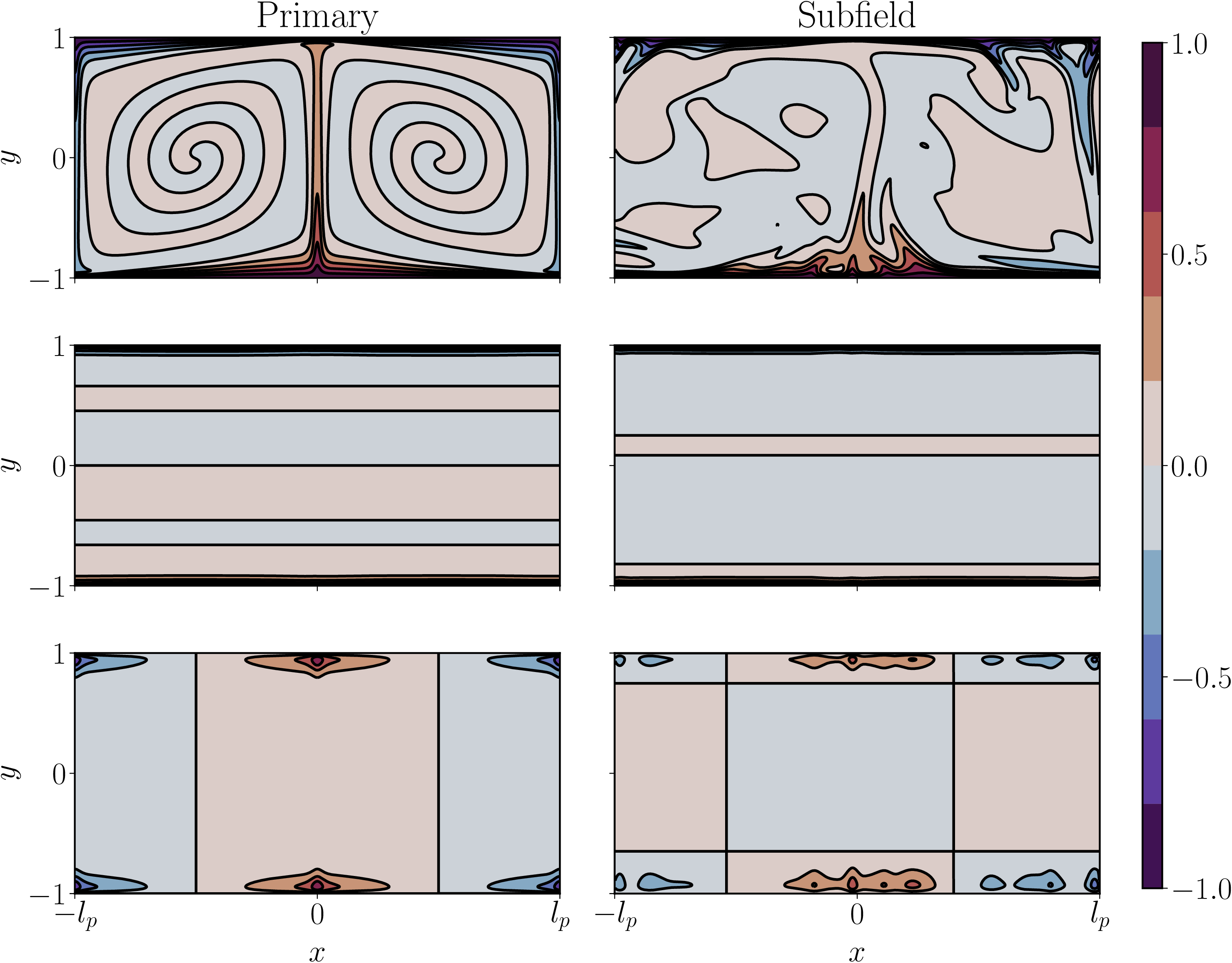
Furthermore, Figure 2 shows the appearance of all three steady solutions — primary, optimal, and local maximum — within a single time snapshot of a simulation with domain aspect ratio , , and . The time is relatively early in the evolution from initial conditions (12) with random amplitudes. Notice that these initial conditions do not select a scale in the horizontal direction, and that the horizontal scales of the primary, optimal and local max arise spontaneously from nonlinear interactions. At this early time , the flow is quasi-steady, and later transitions to a quasi-periodic, statistically steady state. In Figure 2, the middle left, middle right and bottom panels compare, respectively, the optimal, local maximum and primary solution to different simulation sub-boxes. In each case, the sub-box has the same horizontal scale as the corresponding steady solution, e.g., the primary solution has horizontal scale .

Motivated by Figures 1 and 2, the purpose of the current investigation is to explore how transition to turbulence in 2D Rayleigh-Bénard convection is influenced by the primary and optimal steady solutions. We focus on Rayleigh numbers well above the onset of convection and well below the ultimate regime. In this range, the flow is potentially described as a dynamical systems ‘repeller’ consisting of unstable solutions that are sampled by turbulence trajectories [51]. In such a description, solutions with a small number of unstable directions in phase space would be sampled most frequently. With increasing , one would expect more and more unstable (and unsteady) solutions of increasing complexity in the phase space, thus complicating such an investigation at higher . The possibility of describing turbulence as a repeller has been previously explored in the context of wall-bounded shear flows (see [52, 53, 51, 54, 55, 56, 57] and references therein).
We restrict our investigation to and , in part because their optimal solutions are distinct from one another [2]. The optimal thermal fields of cases have coiling arms and a larger wavelength, as compared to those of which are armless and columnar [1, 2]. Furthermore, has the added benefit of having been investigated extensively in the literature. Despite the differences in the nature of the optimal solution for and , the scaling behavior of with is almost identical (see Figure 1). We perform well-resolved numerical simulations and analyze the resulting datasets using two main analysis techniques. First we consider the spatial correlation between the computed steady-state solutions (primary or optimal) and ‘windows’ of the simulation data with the same aspect ratio as the steady-state solution. Second, we use the singular value decomposition on the windows with high correlation to compare the underlying structures. Our work fits within a broader class of data-driven approaches to explore structures and dynamics in Rayleigh-Bénard convection. For example, the dynamic mode decomposition has been used to search turbulence data for unstable periodic orbits [58]. Turbulent superstructures with scale separation were identified in [59]. In [29], a convolutional neural network was trained and used to analyze turbulent superstructures. Constrained generative adversarial neural networks have been used to learn the underlying distribution of a Rayleigh-Bénard convection dataset [60].
The rest of the paper is organized as follows. Section II presents the governing equations and the details of the numerical simulations. Section III describes the methodologies we used to detect the footprint of the steady solutions, and the rationales behind them. The results are presented in Section IV, followed by discussion in Section V.
II Background
II.1 Governing Equations
In Rayleigh-Bénard convection, a fluid under the influence of gravity is contained between two horizontal plates separated by a distance such that the lower plate is held at a higher temperature () than the upper plate (). Buoyancy effects are incorporated into the Navier-Stokes equations via the Oberbeck-Boussinesq approximation [61, 62, 6, 63], wherein density is assumed to vary linearly with temperature in the buoyancy term. In particular, the density variations in the buoyancy term have the form where , is a reference temperature, and is the coefficient of volume expansion of the fluid. In the conduction state, the fluid is quiescent and the temperature conduction profile varies linearly with [64]. For plates situated at such that , the conduction profile is where is the temperature difference between the bottom and top plate. In the present work, we restrict our investigation to two-dimensional flows. We work with a nondimensional form of the equations where temperature is scaled by , length by , time by the free fall time , velocity by the free fall velocity , and pressure by a dynamic pressure . All variables, unless explicitly stated, are understood to be nondimensionalized. The nondimensional governing equations are,
| (1) | |||
| (2) | |||
| (3) |
where is the velocity, is the temperature departure from the conduction state, and is the unit vector in the direction perpendicular to the bottom wall. The nondimensional parameters and are related to the classical and by,
| (4) |
where,
| (5) |
The additional dimensional quantities appearing in the definitions of and are the acceleration due to gravity , the kinematic viscosity , and the thermal diffusivity . We note that in (1) is a modified pressure equal to where is the nondimensional mechanical pressure appearing in the momentum equation and is a nondimensional reference temperature. As a final note, in this nondimensionalization the conduction profile is .
No-slip and fixed temperature boundary conditions are imposed on the plates such that
| (6) |
The domain extends from to in the horizontal direction, with periodic boundary conditions,
| (7) |
Here represents the domain length nondimensionalized by so that the dimensional domain has length .
Figure 3 depicts the problem configuration.

In this geometry, and for the selected nondimensionalization, the domain aspect ratio is . Simulations in this domain are compared to the optimal and primary solutions, which extend from to and to , respectively. The horizontal domain for the optimal and primary structures is therefore where is the half-width of the structure being considered. In subsequent sections, the half-width of a turbulent plume will be denoted by and the context will make it clear if the plume is an optimal, primary, local max or turbulent structure.
Before the onset of convection, the heat transfer depends linearly on the temperature difference between the plates. This linear relation breaks down at the onset of thermal instability as the convective modes of heat transport activate [65]. The conduction solution is found to be linearly unstable when exceeds a critical value of for no-slip boundaries [64, 63]. After convection sets in, the dimensional flux through each of the top and bottom boundaries is given by
| (8) |
where is the horizontal average of temperature. Typically, the dimensionless Nusselt number is used to represent the relative strength of convective heat transfer, where the Nusselt number is defined as the ratio of the total heat flux to the heat flux by pure conduction. For example, using the value of the heat flux at the bottom wall, one can define an instantaneous Nusselt number
| (9) |
With the nondimensionalization introduced above, (9) becomes
| (10) |
and the quantity (10) is used herein for plots of Nusselt number as a function of time. In statistically steady state, the time-averages of and in (8) are equal, and we denote this time average by . Then the time-averaged Nusselt number in statistically steady state is given by . For before the onset of convection, the value of is unity, since all of the heat transferred is by conduction. For , the heat transfer is bolstered by convective effects, and thus .
II.2 Numerical Simulations
Our numerical simulations were performed using the open-source, MPI-parallelized code Dedalus [66, 67, 68], using a Fourier discretization in the horizontal direction and a Cheybshev discretization in the wall-normal direction. Table 1 presents the spatial resolution of selected runs, where () is the number of Fourier (Chebyshev) basis functions used in the -direction (-direction). The rule was used for dealiasing. Also tabulated are features of the optimal solution at the given and , such as the width of the optimal box, and the optimal Nusselt number . The convection in Table 1 is computed as .
Time-integration is accomplished with an adaptive implicit-explicit (IMEX) Runge-Kutta (RK) method. Specifically, we use a method (four implicit stages, four explicit stages, third order accurate) [69]. Moreover, the time-step is adjusted dynamically to ensure that the CFL number is less than unity. To determine when the flow has reached statistically steady state, time averages of were taken over time windows containing 5 (dimensionless) eddy turnover times defined as
| (11) |
where represents a volume average and is the temporal root mean square of the vertical velocity [70]. The eddy turnover time is a measure of the time it takes a fluid parcel to traverse the fluid layer height twice. The flow is considered to be in a statistically steady state once the difference between the successive time averages drops below . In order to balance high fidelity and computational time, all simulations were run for approximately 10 eddy turnover times after attaining statistically steady state. Mesh refinement was performed for the computations presented in Table 1 to ensure that the simulations were well-resolved.
The simulations were initialized from a state of rest, with temperature distribution
| (12) |
where and are random numbers drawn from a normal distribution. The quadratic form in satisfies the boundary conditions at the walls, and the noisy amplitude factor allows us to seed the temperature without imposing any horizontal scale. At low , we found that the stationary state may exhibit sensitivity to initial conditions. For example, in a domain with aspect ratio , and for parameters and , we observed two distinct stationary states—one with 4 plumes in the temperature field (), and the other with 5 plumes (). As will become evident below, for low , the horizontal length scale and spacing of the emerging plumes appears to be heavily influenced by the optimal and primary steady solutions. Sensitivity to initial conditions at low has also been discussed in [71, 72].
As noted above, the number of thermal structures in the temperature field may be influenced by the choice of . Our objective was to allow the nonlinear interactions, rather than the box size, to select the dominant horizontal scale. In [73] and [26], the authors investigated three-dimensional Rayleigh-Bénard convection at and at various aspect ratios. They found that the integral length scale and saturate for, respectively, aspect ratio and . Our 2D studies showed that the scaling of vs. for and is largely insensitive to changes in box size beyond . Thus we chose to help ensure that the intrinsic dynamics are determining the number and spacing of the plumes in steady state (with some sensitivity for low as mentioned).
We also investigated the domain aspect-ratio dependence of the mean flow (the horizontal average of the horizontal velocity ). We observed that the ratio of mean flow energy and total kinetic energy decreases substantially with increase in for , (the energy ratio is at ). The authors in [74] report that the energy contained in the mean flow relative to the total kinetic energy is always less than at for all the cases considered () which includes and . Furthermore, it is observed that the mean flow lowers . Indeed, the primary and optimal solutions have zero mean-flow imposed by symmetry about the -axis. Thus, when searching for the signature of the primary and optimal solutions in the simulation results, the essentially-zero mean flow is an additional motivation for the choice .
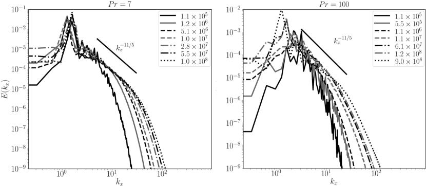
The kinetic energy spectra in statistically steady state are shown in Figure 4. All the reported runs are broad spectrum and therefore have non-trivial flow dynamics. As increases, the developing inertial range is consistent with the scaling [75]. The thermal energy spectra from our simulations also appear to approach the scaling reported in previous studies [76].
III Methodology
When considering strategies to detect steady solutions in the time developing simulations, we first explored approaches to search for the signature of the optimal solutions. An obvious strategy is to monitor the global heat transfer and focus on high instantaneous events. Then, extracting flow fields at individual times corresponding to high , one may inspect these fields for signs of structural similarity with the optimal solutions. Although this method is successful at low , it has a number of drawbacks. First, the global is governed by the combined contributions of all the plumes present in the field at any given time, and therefore may not be the best indicator of a close match between the optimal solution and a local plume in the large-aspect-ratio box. Furthermore, we wish to employ a more general technique to detect different steady solutions (optimal, local max, and primary).
To address these concerns, we developed a windowing technique to search locally for all of the known steady solutions, at all times, keeping and fixed. For fixed time, Figure 5 illustrates the idea using a schematic of the optimal solution for .

By sliding the window across the length of the box, one can compute the spatial correlation between a steady solution and the sub-field centered at , given by
| (13) |
where is an inner product and is the temperature field of the steady solution. The notation refers to the temperature field in a portion of the computational domain, which is centered at location with horizontal extent . Repeating this for every snapshot of the temperature field, one obtains the alignment as a function of position and time . This spatial correlation data can be used to approximate a probability density function, from which we can quantify the likelihood of convective plumes that are highly correlated with a particular steady solution. For a given time regime, e.g. the spin-up period or statistically steady state regime, we counted the number of sub-fields with correlation . We define the incidence parameter as
| (14) |
where is the number of sub-fields within the specified correlation range, and is the total number of sub-fields. A few representative values of the incidence parameter for the primary solution are given in Table 2 and for the optimal solution in Table 3. These numbers will help to inform the discussion in Section IV.
The windowing technique allows us to identify the influence of multiple steady states on the structure and statistics of transitional flows, especially with respect to horizontal scale selection by nonlinear interactions. For this first study, beyond our lowest , we focus on the primary and optimal solutions. We observe that several of their features can remain intact for at both considered in this work. It is remarkable that their signatures endure, since turbulence significantly disrupts their wall-to-wall nature, along with their upright plumes, and in some cases, their delicate interior structures. Once highly-correlated sub-fields have been identified, singular value decomposition [77] is used for more detailed comparison between steady solutions and instantaneous simulation sub-fields. We find that the first two SVD modes are associated with the boundary layer and plume structures, respectively, and provide a quantitative means to separately assess agreement for these two structural features.
IV Results
To set the stage, we begin this section by reviewing some relevant literature describing the dynamics of similar regimes studied herein. In [78], the authors employed a low dimensional model using the most energetic modes from direct numerical simulations to study 2D flow regimes at . According to [78], the flow is chaotic for , where and . Experimental studies in [79] investigated the many routes the flow takes to reach a turbulent state, and the dependence of these routes on aspect ratio , , and the presence of a mean flow. Their results for at show that transition to a non-periodic state occurs for . For , the lowest value of investigated in our simulations is , expected to be well above the threshold for chaos by comparison to [78, 79]. In the experimental studies [34] with at , the flows with have been described as being turbulent.
We also conducted studies of our own to classify the nature of our simulation fields. For example, we examined the time traces of vertical velocity and temperature, collected from probes placed in the bulk and the boundary layer. With the exception of the lowest for , all cases exhibited spectra with a broad wavenumber and frequency distribution in statistically steady state (see Figure 4).
We next present our results, organized into two separate sections for and (Section IV.1 and IV.2, respectively). As we will demonstrate, primary and optimal structures are readily observed in temperature fields corresponding to transitional values of . Visualizations and data analysis of the simulations for higher suggest that a signature of the primary solution persists for , consistent with agreement for vs. scaling seen in Figure 1. The optimal solution for higher is easier to detect in the case of , perhaps in part because of its simpler structure compared to the optimal solution for (see Figure 13).
IV.1
IV.1.1 Visualizations and correlation data
We first present results for transitional ( and ), starting with the time evolution of the instantaneous Nusselt number in Figure 6. After a significant transient period , the system eventually settles to a chaotic statistically steady state for .

In statistically steady state, the Nusselt number is approximately , but one can see large fluctuations in the instantaneous Nusselt number, frequently attaining values greater than of the optimal value . The vs. scaling in agreement with the primary solution (Figure 1), together with the near-optimal, values of (Figure 6), suggest that both primary and optimal solutions may be influencing the structure of the boundary layer in this transitional flow. Hence we investigate this possibility using our windowing technique, followed later by singular value decomposition of the highly correlated fields for closer inspection of the boundary layers. Note that the incidence parameters for the primary and optimal solutions are quite close to each other, and greater than , in both the transient and statistically steady regimes (see Tables 2 and 3).
Figure 7 (middle panel) displays an instantaneous snapshot of the temperature field in the simulation with . The snapshot corresponds to the early time , when different horizontal length scales are emerging from nonlinear interactions, quite clearly corresponding to the scales associated with the primary, optimal and local maximal heat transport solutions (top panel). The situation is similar to Figure 2 for at the same (though the values of are different). In Figure 7, the bottom panel shows two prominent peaks in the correlation function defined by (13) for the optimal solution, roughly located at and . Centered at these locations, there is a temperature plume in the time-developing simulation with visual similarity to the optimal solution, especially with respect to horizontal scale and overall shape (see the top panel for a comparison centered at ). The analogous correlation function for the second maximal heat transport solution has six peaks, and again, one observes overall structural similarity between the steady solution and updrafts in the simulation field. At this early time (), the primary solution is highly correlated with only one temperature plume located at . These observations are consistent with the high values, close to optimal, achieved by the instantaneous Nusselt number during early spin-up times .


As the simulation progresses, the system eventually settles into a statistically steady state with representative temperature field shown on the top panel of Figure 8. At the time shown in the figure, the correlation functions for the optimal and primary solutions (middle panel) both show five distinct peaks corresponding to the temperature updrafts. The bottom left column (bottom right column) compares the optimal (primary) solution and a single plume of the turbulent snapshot centered at . Note that the size of the alignment window is different for the same plume because the window is determined by the horizontal length scale of the optimal or primary solution. The correlation functions show a slightly better match between the primary solution and instantaneous updrafts. From Tables 2 and 3, we also observe that the incidence for the primary solution is roughly higher than the incidence for the optimal solution, after the flow has transitioned to statistically steady state at . The information from the correlation data reflects, in part, the tendency of the nonlinear interactions to select the horizontal scale of the primary solution. As also seen from Tables 2 and 3, while both incidence values decrease for increasing , the gap between the primary solution incidence and the optimal solution incidence grows. That gap is consistent with the vs. data in Figure 1, and also with the spacing of large-scale horizontal plumes as visualized in Figure 9.
We note that the correlation weighs similarities in regions of low and high temperature () more than in the regions with temperatures near zero. Since the same boundary conditions are imposed for the steady solutions and the time-developing flows, necessarily leading to top and bottom boundary layers, the correlations rarely go below the value . Furthermore, the temperature contours of highly correlated structures picked out by the windowing algorithm match well with the thermal structures in the top and bottom boundary layers, rather than in the bulk where the temperature distribution is close to zero. As mentioned above, this must be kept in mind for higher values of , when fluctuations become more vigorous leading to fully developed turbulence. At high , the plumes will not be upright, and interior structures of the steady solutions become fractured, such as the coiling arms of the primary solution (see Figure 12). Indeed, the incidence parameters shown in Tables 2 and 3 decrease accordingly with increasing . Nevertheless, for values of up to , Figure 9 illustrates that very thin ‘plumelets’ converge in the boundary layer to produce larger-scale updrafts that are nearly wall-to-wall, with spacing that appears to be approximately given by the horizontal scale of the primary solution. Figure 9 is a Schlieren-type plot of the function
| (15) |
where is the magnitude of the temperature gradient at each point in the domain, is the maximum temperature gradient magnitude over the domain, and is a scaling parameter. The values of are different in the bulk and boundary layers and specific values are reported along with the accompanying figures. The exponential function helps to bring out flow features [80] that may otherwise be washed out in the visualization. Counting the number of large-scale updrafts in our statistically steady flows for , one consistently arrives at the number (approximately) 5 in the domain of length . Since the width of the primary solution is , this strongly suggests that the horizontal scale selected by the disordered flow is determined by the primary solution, at least in this range of
IV.1.2 Singular Value Decomposition of Steady Solutions and Simulation Sub-fields
Here we further scrutinize the dominant features of simulation sub-fields selected by the windowing algorithm for a more detailed comparison to the steady solutions, either primary or optimal. Standard singular value decomposition (SVD) [77] is used to analyze the temperature field of the steady solutions and the simulation sub-fields. To select a specific sub-field for the SVD analysis, we first isolate sub-fields with correlation values greater than or equal to . These sub-fields are filtered by averaging the temperature profiles in the range , and then selecting those sub-fields with a peak in the averaged temperature in the range , where the length of the sub-field is . The specific instances for SVD are chosen blindly from this subset. Note that this algorithm can select sub-fields with lower correlation value than those counted in the incidence parameter (14).

In Figure 10, we compare the singular values of the first 5 SVD modes for three cases: (primary and optimal) and (primary). In each case, the simulation sub-fields correspond to the statistically steady time regime. As is traditional, one may interpret each singular value as an ‘energy,’ and the sum over all values as the total energy. The ratio is interpreted as the percent of energy in any given SVD mode with number . As can be seen the figure, roughly of the total energy is contained in SVD modes 1 and 2. For the same three cases, Figures 11-12 show that these two SVD modes correspond to, respectively, the boundary layer and updraft-downdraft structures of both steady solutions and simulation sub-fields. The SVD analysis provides an additional quantitative comparison of these structures, adding to the vs. information in Figure 1, and the correlation data provided in the previous section.

| Relative Error | Relative Error | |||||
|---|---|---|---|---|---|---|
| (primary) | % | |||||
| (optimal) | ||||||
| (primary) |
For , Figure 11 shows contour plots of the 1st and 2nd SVD modes of the primary and optimal solutions, compared with highly-correlated simulation sub-fields. The left two columns present the comparison of the primary solution to a simulation sub-field with correlation . For the first mode corresponding to the boundary layer, the absolute error over the domain ranges between in the boundary layer to in the middle of the domain. Near the boundary layer, the first SVD mode of the primary solution is in remarkably good agreement with the first SVD mode of the turbulent plume. Contour plots of the absolute error are given in Figure 20 of Appendix A. We also note that a typical value of the absolute error is in the boundary layer [] and in the bulk []. The second mode corresponding to the updraft-downdraft exhibits a similarly good agreement (Figure 11 and Figure 20 in Appendix A). Comparing contours of the same levels, SVD mode 1 reveals an extremely close match between boundary layer thicknesses for the primary solution and the simulation window. To make this comparison quantitative, Table 4 presents the normalized singular values for SVD mode 1, where the relative error reflects agreement between the boundary layer heights. Notice the small relative error value of for SVD mode 1 analysis of the primary solution at .
The right two columns of Figure 11 present the comparison between SVD modes for the optimal solution and a simulation sub-field with correlation . Once again, the first SVD mode corresponds to the boundary layer, however, the agreement is not as close as observed for the primary solution comparison. Figure 21 in Appendix A provides contours of the absolute error for this case. The boundary layer in the optimal solution is smaller than the boundary layer of its companion sub-field, and Table 4 gives a relative error of . Since scales with the reciprocal of the boundary layer thickness, this observation is consistent with Figure 1, in which provides an upper bound on for the primary and turbulent solutions. As an upper bound on heat transport, the optimal steady solution necessarily has thinner boundary layer than the average boundary layer thickness in the simulation domain. The rather tight nature of the bound, especially at transitional values of , is captured by the SVD mode 1 analysis of highly correlated simulation windows with the optimal length scale.
We finish this section with Figure 12, which illustrates how the primary solution persists at higher , albeit with unstable boundary layer, and only distant remnants of the coiling arms. The location of the simulation sub-field is shown by the arrow in the 3rd panel of Figure 9. As can be seen even more clearly from Figure 12 than from Figure 9, two important features of the primary solution remain intact: a boundary layer (1st SVD mode), and the horizontal scale associated with an updraft-downdraft pair (2nd SVD mode). In place of the plume-like structures associated with the 2nd mode at (Figure 11), now the 2nd mode could be described as the ‘hotspots’ (‘cold pools’) at the upwellings (downwellings) of temperature.

IV.2
The results for are similar to those for described in the previous section. On the other hand, for , the windowing technique is able to detect embedded optimal solutions for higher up to . The latter result is consistent with Figure 1, showing that the simulation data has values of closer to the optimal values. Furthermore the best-fit scaling gives exponent for the simulation data, closer to the optimal exponent than to the primary exponent . Two possible reasons for the stronger signature of the optimal solution at compared to are (i) a larger horizontal scale separation between primary and optimal solutions at , and (ii) the simpler interior structure of the optimal solution for . Figure 13 shows the structure of the steady solutions at . The top (bottom) row compares the primary (optimal) solutions for and ; the 1st (2nd) column contrasts primary and optimal solutions for fixed (). One can see that there is a much larger scale separation between primary and optimal solutions for than for at , possibly enhancing our ability to detect the optimal solution at small scales, while observing a signature of the primary solution at larger scales. Furthermore,the optimal structure has a significantly simpler interior structure than the optimal solution for . With these pictures in mind, one main objective of this section will be to identify the optimal solution as a persistent small-scale feature for in the range .
IV.2.1 Visualizations and correlation data
Figure 14 shows the instantaneous Nusselt number vs. for , (, .

Three distinct regimes are present: (i) a transient regime which is quasi-steady, with decreasing ; (ii) a second transient regime ; and (iii) a statistically steady state starting at . Regime (iii) was classified as quasi-periodic by observing multiple distinct peaks in the frequency spectrum corresponding to a velocity probe in the middle of the flow field. In the statistically steady regime, the Nusselt number has the value , compared to the values for the optimal and the primary solution (see also Figure 1).


Representative temperature fields for each of the three time regimes are shown in Figure 15, along with the value of the correlation at each point in the domain for the different solutions: primary, optimal and local-max. Very high correlation coefficients appear frequently for the flow in the quasi-steady and transient regions. Notice, for example, the nearly perfect correlation with the optimal solution at , (top panel). The optimal solutions have higher incidence than the primary solutions at early times (see Table 2 and Table 3). In the statistically steady (quasi-periodic) regime, the incidence values for optimal and primary solutions are both roughly , but the correlation values are slightly higher for the primary solution, and indeed the dominant structures look like modulated versions of the primary solution (see the bottom panel of Figure 15).
As the Rayleigh number is increased beyond transitional values, the Schlieren-type visualizations in Figure 16 show a signature of the primary solution at larger scales, and a boundary layer erupting with many thin plumelets. The scale separation is becoming more obvious for higher , for example at our highest . Our windowing technique and SVD analysis allow us to compare the plumelets to the low-aspect-ratio optimal solutions, comparison of which follows below. For and , the arrows in Figure 16 identify two of the plumelets to be analyzed in Section IV.2.2.
IV.2.2 SVD Analysis of Small-Scale Structures
Similarly to section IV.1.2, in this section we perform the SVD on highly correlated subfields and their corresponding optimal solution. Figure 17 compares the singular values of the first 5 SVD modes for three optimal solutions and their corresponding highly-correlated subfields: , , and .

In all three cases, the first 2 modes of the SVD contain greater than of the total energy. Figure 18 shows contour plots of the 1st and 2nd SVD modes of the optimal solutions compared with the highly-correlated subfields at (left two columns), (middle two columns), and (right two columns).

| Relative Error | Relative Error | |||||
|---|---|---|---|---|---|---|
| (optimal) | % | |||||
| (optimal) | ||||||
| (optimal) |
The simulation sub-fields used in the comparison have at , at , and at . Similarly to the case, the 1st SVD mode selects the boundary layer. For , the 1st SVD mode of the optimal solution looks qualitatively similar to the 1st SVD mode of the turbulent sub-field up to . Table 5 presents the relative errors in the 1st and 2nd singular values between the optimal solution and turbulent sub-fields. The relative errors in the first singular values remain remarkably low up to .
For the high , it is interesting to note that the relative error for SVD mode 1 is only (Table 5 and Figure 18). To better appreciate the match, Figure 22 in Appendix A is the same comparison between optimal solution and turbulent sub-box presented in the top row, third column of Figure 18, but with a flattened aspect ratio to visualize the small, blunt plumelet emanating from bottom boundary. The resemblance of the optimal and turbulent structures is quite striking. Contour plots of the absolute error for the 1st mode are presented in Figure 23 in Appendix A. The absolute error in the domain ranges between in the boundary layer to in the bulk region. Typical values are in the boundary layer [] and in the bulk []. We note that at , the errors in the 2nd SVD mode are considerably larger, reaching order one.
V Conclusions
We investigated a transitional range of Rayleigh numbers for and to find signatures of 2D steady solutions that were first described in [1] and [2]. These steady solutions satisfy no-slip boundary conditions in the wall-normal direction, periodic boundary conditions in the horizontal direction, and were found by numerical continuation as bifurcations from the conduction state at . The primary solution has aspect ratio , and becomes unstable at to a time-periodic solution. The optimal solution maximizes heat transport over steady solutions, and has aspect ratio that decreases with increasing . A third type of steady solution corresponds to a local maximum of the heat transport, also with aspect ratio smaller than . These solutions impose mirror symmetry about , and generally speaking, their temperature fields consist of one hot/cold plume pair, with the hot plume emanating from the bottom boundary layer and centered at . On the other hand, the three solution types differ with respect to details such as horizontal scale, boundary layer thickness and interior structure.
A domain aspect ratio was chosen for the simulations in the current work, allowing multiple copies of coherent structures reminiscent of the steady solutions to appear spontaneously from nonlinear interactions, with minimal constraint by the domain dimensions. The simulation data for vs. is almost coincident with the data for the primary solution at at these relatively low values , especially at the lower end of the range (Figure 1). For , the primary solution becomes less relevant with increasing , and the optimal scaling appears to be more dominant. Thus, from the outset, the statistical data strongly suggested a structural relevance of the primary solution for transition to turbulence. At the same time, the tight upper bound on provided by the optimal solution inspired us ask if the optimal solution might also influence the features of transitional and turbulent data (Figures 1, 6 and 14).
Our objective was to establish further links between the simulation data and the steady solutions, beyond the vs. information, and for two regimes of represented by and . In particular, we used a moving window technique to identify simulation sub-fields with high correction coefficient (13), considering all three types of steady solutions for the comparison at . As evidenced by Figures 2, 7, and 15, the results are stunning, with all three steady solutions appearing prominently during transition to statistically steady state. Then, as the flows enter the statistically steady time regime, a modulated version of the primary solution is dominant. For higher , we focused on the primary and optimal solutions, leaving further study of local maximal transport solutions for future work.
For in the two decades , Schlieren-type plots – Figure 9 ( and Figure 16 () – show a multi-scale horizontal structure in the simulation snapshots. Visual inspection suggests that the primary solution sets the large horizontal scale of turbulent plumes, and the intriguing possibility for the optimal solution to impact the small-scale plumelets that converge together in a primary-scale updraft. We investigated these large-scale and small-scale features using singular value decomposition on highly-correlated sub-fields and, respectively, their corresponding primary and optimal solutions.
Consistent with the vs. plots in Figure 1, we found subtle differences in the dominance of the primary solutions at large scales, and the persistence of the optimal solutions at small scales. For , the windowing technique and SVD analyses clearly identify the primary solution as embedded within the turbulence at (Figure 12), while the signature of the optimal solution is much less apparent. We note the lack of scale separation between primary and optimal solutions for at the moderate value (Figure 13). On the other hand, there is a definitive scale separation between primary and optimal solutions for , , and the analyses favor the optimal solutions (Figure 18). It is conceivable that larger scale separation between primary and optimal solutions will facilitate detection techniques aimed at higher regimes.
An interesting possibility is presented by the high- 2D simulation data of [38] in the range In a box of aspect ratio and for , [38] find an approximate scaling vs. with for , beyond which they report a transition to [38, 39, 81]. Their data is reproduced here in Figure 19, along with (i) our lower data for , and ; (ii) the primary solution best-fit scaling at extended to the range ; and (iii) the optimal solution best-fit scaling at extended to the range . One can see a seamless transition between our 2D data for and the 2D data for [38]. Furthermore, the continuation of the optimal scaling with begs the question as to whether or not the transition in 2D exponent at [38] could be related to boundary-layer structures with horizontal and vertical scales determined by the optimal solution. Thus, it would undoubtedly be revealing to pursue higher values of in 2D, along with application of other types of data analyses ([82, 83, 29, 84, 60, 85]), in the exploration of exact coherent solutions.
Figure 19 also reproduces the 3D data recently computed for up to in [30]. One can see that the extended optimal scaling for [2] provides a tight upper bound on the high- 3D data, with evidence for tendency toward the same scaling exponent as increases. As has previously been suggested [1, 2], it remains to uncover a possible connection between the 2D optimal solutions and the 3D data. Finally, work to numerically compute exact solutions in 3D is ongoing [28, 86], and a longer-term goal is to explore the relevance of 2D and 3D exact solutions to 3D turbulence.

Acknowledgements
The authors thank Charles Doering, Andre Souza and Fabian Waleffe for helpful feedback during the development of this work. Fabian Waleffe also contributed suggestions for the written manuscript leading to significant improvements.
References
- Waleffe et al. [2015] F. Waleffe, A. Boonkasame, and L. M. Smith, Heat transport by coherent Rayleigh-Bénard convection, Physics of Fluids (1994-present) 27, 051702 (2015).
- Sondak et al. [2015] D. Sondak, L. M. Smith, and F. Waleffe, Optimal heat transport solutions for Rayleigh–Bénard convection, Journal of Fluid Mechanics 784, 565 (2015).
- Lappa [2009] M. Lappa, Thermal convection: patterns, evolution and stability (John Wiley & Sons, 2009).
- Rajagopal et al. [1996] K. R. Rajagopal, M. Ruzicka, and A. R. Srinivasa, On the Oberbeck-Boussinesq approximation, Mathematical Models and Methods in Applied Sciences 6, 1157 (1996).
- Ahlers et al. [2009] G. Ahlers, S. Grossmann, and D. Lohse, Heat transfer and large scale dynamics in turbulent Rayleigh-Bénard convection, Reviews of Modern Physics 81, 503 (2009).
- Chillà and Schumacher [2012] F. Chillà and J. Schumacher, New perspectives in turbulent Rayleigh-Bénard convection, The European Physical Journal E: Soft Matter and Biological Physics 35, 1 (2012).
- Niemela et al. [2000] J. Niemela, L. Skrbek, K. Sreenivasan, and R. Donnelly, Turbulent convection at very high Rayleigh numbers, Nature 404, 837 (2000).
- Chavanne et al. [2001] X. Chavanne, F. Chilla, B. Chabaud, B. Castaing, and B. Hebral, Turbulent Rayleigh-Bénard convection in gaseous and liquid He, Physics of Fluids 13, 1300 (2001).
- Niemela and Sreenivasan [2006] J. Niemela and K. Sreenivasan, Turbulent convection at high Rayleigh numbers and aspect ratio 4, Journal of Fluid Mechanics 557, 411 (2006).
- He et al. [2012a] X. He, D. Funfschilling, E. Bodenschatz, and G. Ahlers, Heat transport by turbulent Rayleigh-Bénard convection for 0.8 and : Ultimate-state transition for aspect ratio , New Journal of Physics 14, 063030 (2012a).
- He et al. [2012b] X. He, D. Funfschilling, H. Nobach, E. Bodenschatz, and G. Ahlers, Transition to the ultimate state of turbulent Rayleigh-Bénard convection, Physical Review Letters 108, 024502 (2012b).
- Bouillaut et al. [2019] V. Bouillaut, S. Lepot, S. Aumaître, and B. Gallet, Transition to the ultimate regime in a radiatively driven convection experiment, Journal of Fluid Mechanics 861 (2019).
- Malkus [1954] W. Malkus, The heat transport and spectrum of thermal turbulence, Proceedings of the Royal Society of London. Series A. Mathematical and Physical Sciences 225, 196 (1954).
- Priestley [1954] C. Priestley, Convection from a large horizontal surface, Australian Journal of Physics 7, 176 (1954).
- Kraichnan [1962] R. Kraichnan, Turbulent thermal convection at arbitrary Prandtl number, Physics of Fluids 5, 1374 (1962).
- Spiegel [1963] E. A. Spiegel, A generalization of the mixing-length theory of turbulent convection., The Astrophysical Journal 138, 216 (1963).
- Howard [1963] L. Howard, Heat transport by turbulent convection, Journal of Fluid Mechanics 17, 405 (1963).
- Busse [1969] F. Busse, On Howard’s upper bound for heat transport by turbulent convection, Journal of Fluid Mechanics 37, 457 (1969).
- Grossmann and Lohse [2000] S. Grossmann and D. Lohse, Scaling in thermal convection: a unifying theory, Journal of Fluid Mechanics 407, 27 (2000).
- Grossmann and Lohse [2002] S. Grossmann and D. Lohse, Prandtl and Rayleigh number dependence of the Reynolds number in turbulent thermal convection, Physical Review E 66, 016305 (2002).
- Doering and Constantin [1994] C. Doering and P. Constantin, Variational bounds on energy dissipation in incompressible flows: Shear flow, Physical Review E 49, 4087 (1994).
- Constantin and Doering [1995] P. Constantin and C. Doering, Variational bounds on energy dissipation in incompressible flows. II. Channel flow, Physical Review E 51, 3192 (1995).
- Doering and Constantin [1996] C. Doering and P. Constantin, Variational bounds on energy dissipation in incompressible flows. III. Convection, Physical Review E 53, 5957 (1996).
- Kerswell [2001] R. Kerswell, New results in the variational approach to turbulent Boussinesq convection, Physics of Fluids 13, 192 (2001).
- Ding and Kerswell [2020] Z. Ding and R. R. Kerswell, Exhausting the background approach for bounding the heat transport in Rayleigh-Bénard convection, Journal of Fluid Mechanics 889, DOI: 10.1017/jfm.2020.41 (2020).
- Bailon-Cuba et al. [2010] J. Bailon-Cuba, M. Emran, and J. Schumacher, Aspect ratio dependence of heat transfer and large-scale flow in turbulent convection, Journal of Fluid Mechanics 655, 152 (2010).
- Emran and Schumacher [2015] M. Emran and J. Schumacher, Large-scale mean patterns in turbulent convection, Journal of Fluid Mechanics 776, 96 (2015).
- Motoki et al. [2018] S. Motoki, G. Kawahara, and M. Shimizu, Maximal heat transfer between two parallel plates, Journal of Fluid Mechanics 851 (2018).
- Fonda et al. [2019] E. Fonda, A. Pandey, J. Schumacher, and K. R. Sreenivasan, Deep learning in turbulent convection networks, Proceedings of the National Academy of Sciences 116, 8667 (2019).
- Iyer et al. [2020] K. P. Iyer, J. D. Scheel, J. Schumacher, and K. R. Sreenivasan, Classical 1/3 scaling of convection holds up to , Proceedings of the National Academy of Sciences 117, 7594 (2020).
- Kawano et al. [2020] K. Kawano, S. Motoki, M. Shimizu, and G. Kawahara, Ultimate heat transfer inwall-bounded’convective turbulence, arXiv preprint arXiv:2004.08831 (2020).
- Wang et al. [2020] Q. Wang, R. Verzicco, D. Lohse, and O. Shishkina, Multiple states in turbulent large-aspect ratio thermal convection: What determines the number of convection rolls?, arXiv preprint arXiv:2005.04535 (2020).
- Sondak et al. [2020] D. Sondak, T. M. Smith, R. P. Pawlowski, S. Conde, and J. N. Shadid, High Rayleigh number variational multiscale large eddy simulations of Rayleigh-Bénard convection, arXiv preprint arXiv:2005.10153 (2020).
- Xia et al. [2002] K.-Q. Xia, S. Lam, and S.-Q. Zhou, Heat-flux measurement in high-Prandtl-number turbulent Rayleigh-Bénard convection, Physical Review Letters 88, 064501 (2002).
- Ahlers et al. [2017] G. Ahlers, E. Bodenschatz, and X. He, Ultimate-state transition of turbulent Rayleigh-Bénard convection, Physical Review Fluids 2, 054603 (2017).
- Doering [2019] C. R. Doering, Thermal forcing and ‘classical’ and ‘ultimate’ regimes of Rayleigh–Bénard convection, Journal of Fluid Mechanics 868, 1 (2019).
- Stevens et al. [2018a] R. Stevens, R. Verzicco, and D. Lohse, Direct numerical simulations towards ultimate turbulence, Bulletin of the American Physical Society (2018a).
- Zhu et al. [2018] X. Zhu, V. Mathai, R. J. Stevens, R. Verzicco, and D. Lohse, Transition to the ultimate regime in two-dimensional Rayleigh-Bénard convection, Physical Review Letters 120, 144502 (2018).
- Doering et al. [2019] C. R. Doering, S. Toppaladoddi, and J. S. Wettlaufer, Absence of evidence for the ultimate state of turbulent Rayleigh-Bénard convection, Physical Review Letters 123, 259401 (2019).
- Doering [2020] C. R. Doering, Turning up the heat in turbulent thermal convection, Proceedings of the National Academy of Sciences 117, 9671 (2020).
- Grossmann and Lohse [2004] S. Grossmann and D. Lohse, Fluctuations in turbulent Rayleigh–Bénard convection: the role of plumes, Physics of Fluids 16, 4462 (2004).
- Stevens et al. [2013] R. Stevens, E. van der Poel, S. Grossmann, and D. Lohse, The unifying theory of scaling in thermal convection: The updated prefactors, Journal of Fluid Mechanics 730, 295 (2013).
- Whitehead and Doering [2011] J. Whitehead and C. Doering, Ultimate state of two-dimensional Rayleigh-Bénard convection between free-slip fixed-temperature boundaries, Physical Review Letters 106, 244501 (2011).
- Hassanzadeh et al. [2014] P. Hassanzadeh, G. Chini, and C. Doering, Wall to wall optimal transport, Journal of Fluid Mechanics 751, 627 (2014).
- Whitehead and Wittenberg [2014] J. Whitehead and R. Wittenberg, A rigorous bound on the vertical transport of heat in Rayleigh-Bénard convection at infinite Prandtl number with mixed thermal boundary conditions, Journal of Mathematical Physics 55, 093104 (2014).
- Choffrut et al. [2016] A. Choffrut, C. Nobili, and F. Otto, Upper bounds on Nusselt number at finite Prandtl number, Journal of Differential Equations 260, 3860 (2016).
- Otto et al. [2017] F. Otto, S. Pottel, and C. Nobili, Rigorous bounds on scaling laws in fluid dynamics, in Mathematical Thermodynamics of Complex Fluids (Springer, 2017) pp. 101–145.
- Doering et al. [2006] C. Doering, F. Otto, and M. Reznikoff, Bounds on vertical heat transport for infinite-Prandtl-number Rayleigh-Bénard convection, Journal of Fluid Mechanics 560, 229 (2006).
- Wang [2007] X. Wang, Asymptotic behavior of the global attractors to the Boussinesq system for Rayleigh-Bénard convection at large Prandtl number, Communications on Pure and Applied Mathematics 60, 1293 (2007).
- Otto and Seis [2011] F. Otto and C. Seis, Rayleigh-Bénard convection: Improved bounds on the Nusselt number, J. Math. Phys. 52, 083702 (2011).
- Gibson et al. [2008] J. Gibson, J. Halcrow, and P. Cvitanović, Visualizing the geometry of state space in plane Couette flow, Journal of Fluid Mechanics 611, 107 (2008).
- Nagata [1990] M. Nagata, Three-dimensional finite-amplitude solutions in plane Couette flow: bifurcation from infinity, Journal of Fluid Mechanics 217, 519 (1990).
- Waleffe [2001] F. Waleffe, Exact coherent structures in channel flow, Journal of Fluid Mechanics 435, 93 (2001).
- Viswanath [2008] D. Viswanath, The dynamics of transition to turbulence in plane Couette flow, in Mathematics and Computation, a Contemporary View (Springer, 2008) pp. 109–127.
- Hall and Sherwin [2010] P. Hall and S. Sherwin, Streamwise vortices in shear flows: harbingers of transition and the skeleton of coherent structures, Journal of Fluid Mechanics 661, 178 (2010).
- Eckhardt et al. [2007] B. Eckhardt, T. M. Schneider, B. Hof, and J. Westerweel, Turbulence transition in pipe flow, Ann. Rev. Fluid Mech. 39, 447 (2007).
- Chini [2016] G. Chini, Exact coherent structures at extreme Reynolds number, Journal of Fluid Mechanics 794, 1 (2016).
- Page and Kerswell [2019] J. Page and R. R. Kerswell, Searching turbulence for periodic orbits with dynamic mode decomposition, arXiv preprint arXiv:1906.01310 (2019).
- Pandey et al. [2018] A. Pandey, J. D. Scheel, and J. Schumacher, Turbulent superstructures in Rayleigh-Bénard convection, Nature communications 9, 1 (2018).
- Wu et al. [2020] J.-L. Wu, K. Kashinath, A. Albert, D. Chirila, H. Xiao, et al., Enforcing statistical constraints in generative adversarial networks for modeling chaotic dynamical systems, Journal of Computational Physics 406, 109209 (2020).
- Oberbeck [1879] A. Oberbeck, Über die wärmeleitung der flüssigkeiten bei berücksichtigung der strömungen infolge von temperaturdifferenzen, Annalen der Physik 243, 271 (1879).
- Boussinesq [1903] J. Boussinesq, Théorie analytique de la chaleur, Vol. 2 (Gauthier-Villars, 1903).
- Chandrasekhar [2013] S. Chandrasekhar, Hydrodynamic and Hydromagnetic Stability (Courier Dover Publications, 2013).
- Drazin and Reid [2004] P. Drazin and W. Reid, Hydrodynamic Stability (Cambridge university press, 2004).
- Schmidt and Milverton [1935] R. Schmidt and S. Milverton, On the instability of a fluid when heated from below, Proceedings of the Royal Society of London. Series A-Mathematical and Physical Sciences 152, 586 (1935).
- Burns et al. [2020] K. J. Burns, G. M. Vasil, J. S. Oishi, D. Lecoanet, and B. P. Brown, Dedalus: A flexible framework for numerical simulations with spectral methods, Physical Review Research 2, 023068 (2020).
- Lecoanet et al. [2015] D. Lecoanet, M. Le Bars, K. J. Burns, G. M. Vasil, B. P. Brown, E. Quataert, and J. S. Oishi, Numerical simulations of internal wave generation by convection in water, Physical Review E 91, 063016 (2015).
- Couston et al. [2018] L.-A. Couston, D. Lecoanet, B. Favier, and M. Le Bars, The energy flux spectrum of internal waves generated by turbulent convection, Journal of Fluid Mechanics 854 (2018).
- Ascher et al. [1995] U. Ascher, S. Ruuth, and B. Wetton, Implicit-explicit methods for time-dependent partial differential equations, SIAM Journal on Numerical Analysis 32, 797 (1995).
- Sakievich et al. [2016] P. Sakievich, Y. Peet, and R. Adrian, Large-scale thermal motions of turbulent rayleigh–bénard convection in a wide aspect-ratio cylindrical domain, International Journal of Heat and Fluid Flow 61, 183 (2016).
- Venturi et al. [2010] D. Venturi, X. Wan, and G. E. Karniadakis, Stochastic bifurcation analysis of Rayleigh–Bénard convection, Journal of Fluid Mechanics 650, 391 (2010).
- van der Poel et al. [2011] E. P. van der Poel, R. J. Stevens, and D. Lohse, Connecting flow structures and heat flux in turbulent Rayleigh-Bénard convection, Physical Review E 84, 045303 (2011).
- Stevens et al. [2018b] R. J. Stevens, A. Blass, X. Zhu, R. Verzicco, and D. Lohse, Turbulent thermal superstructures in Rayleigh-Bénard convection, Physical Review Fluids 3, 041501 (2018b).
- Hartlep et al. [2003] T. Hartlep, A. Tilgner, and F. Busse, Large scale structures in Rayleigh-Bénard convection at high Rayleigh numbers, Physical Review Letters 91, 064501 (2003).
- Mishra and Verma [2010] P. K. Mishra and M. K. Verma, Energy spectra and fluxes for Rayleigh-Bénard convection, Physical Review E 81, 056316 (2010).
- Chillá et al. [1993] F. Chillá, S. Ciliberto, C. Innocenti, and E. Pampaloni, Boundary layer and scaling properties in turbulent thermal convection, Il Nuovo Cimento D 15, 1229 (1993).
- Trefethen and Bau III [1997] L. Trefethen and D. Bau III, Numerical Linear Algebra, Vol. 50 (Siam, 1997).
- Paul et al. [2011] S. Paul, P. Wahi, and M. K. Verma, Bifurcations and chaos in large-Prandtl number Rayleigh-Bénard convection, International Journal of Non-Linear Mechanics 46, 772 (2011).
- Gollub and Benson [1980] J. Gollub and S. Benson, Many routes to turbulent convection, Journal of Fluid Mechanics 100, 449 (1980).
- Quirk [1997] J. J. Quirk, A contribution to the great Riemann solver debate, in Upwind and High-Resolution Schemes (Springer, 1997) pp. 550–569.
- Zhu et al. [2020] X. Zhu, V. Mathai, R. J. Stevens, R. Verzicco, and D. Lohse, Reply to “Absence of evidence for the ultimate regime in two-dimensional Rayleigh-Bénard convection”, Physical Review Letters 123, 259402 (2020).
- Lee and Carlberg [2018] K. Lee and K. Carlberg, Model reduction of dynamical systems on nonlinear manifolds using deep convolutional autoencoders, arXiv preprint arXiv:1812.08373 (2018).
- Gonzalez and Balajewicz [2018] F. J. Gonzalez and M. Balajewicz, Deep convolutional recurrent autoencoders for learning low-dimensional feature dynamics of fluid systems, arXiv preprint arXiv:1808.01346 (2018).
- Chen et al. [2019] X. Chen, X. Zhu, and M. Brenner, Machine learning meets mechanism: Mechanism of roll reversal in Rayleigh-Bénard convection, Bulletin of the American Physical Society (2019).
- Pandey and Schumacher [2020] S. Pandey and J. Schumacher, Reservoir computing model of two-dimensional turbulent convection, arXiv preprint arXiv:2001.10280 (2020).
- Motoki et al. [2020] S. Motoki, G. Kawahara, and M. Shimizu, Multi-scale steady solution for Rayleigh-Bénard convection, arXiv preprint arXiv:2004.06868 (2020).
Appendix A Supplementary Figures


