Collision Avoidance for Elliptical Agents with Control Barrier Function Utilizing Supporting Lines
Abstract
This paper presents a collision avoidance method for elliptical agents traveling in a two-dimensional space. We first formulate a separation condition for two elliptical agents utilizing a signed distance from a supporting line of an agent to the other agent, which renders a positive value if two ellipses are separated by the line. Because this signed distance could yield a shorter length than the actual distance between two ellipses, the supporting line is rotated so that the signed distance from the line to the other ellipse is maximized. We prove that this maximization problem renders the signed distance equivalent to the actual distance between two ellipses, hence not causing the conservative evasive motion. Then, we propose the collision avoidance method utilizing novel control barrier functions incorporating a gradient-based update law of a supporting line. The validity of the proposed methods is evaluated in the simulations.
I INTRODUCTION
Guaranteeing collision avoidance in multi-agent systems is of significant importance to ensuring safety in many application fields, including environmental monitoring [1, 2], autonomous transportation [3, 4], robot navigation [5], and precision agriculture [6]. In these challenging and complex realms, multi-agent systems are demanded to embrace agents of different capabilities, shapes, and sizes to enhance performance [7]. In the presence of such heterogeneity, the collision avoidance protocol should guide agents not to collide with each other while incorporating their forms.
To achieve real-time collision avoidance for multi-agent systems, various approaches have been developed, including the methods utilizing artificial potential fields (APFs) [8] and control barrier functions (CBFs) [9]. APFs were first presented in [10], and have been employed to the multi-agent systems in the context of the formation [11] and flocking control [12, 13], where a repulsive potential function is designed for steering agents not to collide with each other. A local repulsive function activated only in the sensing regions of each agent is proposed in [14]. On the other hand, CBFs were recently proposed in [15], which confines the state of the system in the set defined by the CBFs. The work [16] developed the collision avoidance methods for multi robot systems, which can be implemented in a distributed fashion. The authors in [17] developed the hybrid CBFs to achieve the collision avoidance of the agents with limited sensing ranges. The comparative study of APFs and CBFs in obstacle avoidance scenarios is conducted in [18]. Most of the mentioned papers assume the agent as a single point, a circular disk, or a sphere. Although these methods can be employed to any agents by overestimating the original shape of agents to a sphere enclosing them, this approach could render too conservative evasive behavior if they have a nonspherical, especially elongated, body.
To mitigate this conservativeness, we propose the collision avoidance method capable of embracing the agents with heterogeneous elliptical shapes, as shown in Fig. 1. Because the CBF provides the ability to synthesize the number of safety-critical constraints [19], e.g., the constraints ensuring the battery of the robot never depletes [20], together with the collision avoidance, we opt for a CBF-based approach. While, in the context of APFs, the work [21] proposes the flocking control for ellipsoidal agents with achieving collision avoidance, the condition used for repulsive potential functions becomes complicated and is not straightforwardly extendable to CBFs. The work [22] employs the result in the computer graphics field to develop the separation condition of elliptical agents. However, the physical interpretation of the metric utilized in the collision avoidance law is not readily understandable since it does not provide the distance between agents. The extent-compatible CBF is developed in [23], where it can prevent the collision among agents having volume by solving a sum-of-squares optimization (SOS) program. Although this method can be applied to elliptical agents, the computational burden stemming from SOS programs might prevent implementations to high order systems. The work also proposes the sampling-based methods while the designer needs to assume the bounded control input. The complexities and limitations in the existing collision avoidance methods for elliptical agents partially come from the difficulties in measuring the distance between two separated ellipses. Although the computational methods deriving numerical solutions of the distance between two ellipses are proposed in the computer graphics field [24, 25], the analytical solution of the distance is difficult to derive in a simple form.
To alleviate the difficulties of evaluating a distance between two ellipses, we propose a novel CBF that incorporates a signed distance from a supporting line of an elliptical agent to the other agent, as illustrated in Fig. 2. Because a naive selection of the supporting line could yield a shorter length than the actual distance between two ellipses, we propose a gradient ascent-based update law, where the supporting line is rotated on the boundary so that the distance between the line and the other ellipse is maximized. We then prove that the maximum value derived from this optimization problem is equivalent to the actual distance between two ellipses. A novel CBF incorporating the gradient ascent input to rotate the supporting line is designed. In addition, we prove that the proposed CBF is a valid one, namely, there always exists the control input to make the collision-free set forward invariance. Numerical simulations demonstrate that the proposed method achieves the collision avoidance between elliptical agents without exhibiting conservative evasive motions.
II Preliminary
II-A Problem Formulation
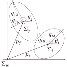
In this paper, we present a collision avoidance method among elliptical agents, labeled through the index set , in 2-D Euclidean space , as illustrated in Fig. 1. We denote the world coordinate frame as . We also define the coordinate frame of agent as , arranged at the center of agent so that its -axis corresponds with the major axis of the ellipse. The relative pose of with respect to is described as with the position and the orientation
| (1) |
The state of agent is defined as . We suppose that the motion of agent can be represented according to a single integrator dynamics,
| (2) |
with the velocity input and the angular velocity input . We denote the control input for agent as . Agent occupies the elliptical region described as
| (3) |
where the constant matrix is defined with and which specify the length of the major axis and the minor axis.
We propose a control method that prevents a collision between elliptical agents described with (3). If the minimum distance between and is described as , the safe set restricting collisions between agents and can be captured by the set
| (4) |
where this set has to be rendered forward invariant. For this goal, we leverage control barrier functions (CBFs) being introduced in the next subsection.
II-B Control Barrier Functions
CBFs have been utilized for ensuring the forward invariance property to the set , in which the state should be confined during the task execution of agents. We assume that a set can be expressed as the superlevel set of a continuously differentiable function , namely, . Then, CBF is defined as follows.
Definition 1.
[15, Def. 5] Given the control affine system
| (5) |
where and are locally Lipschitz, and , together with the set . Then, the function is a control barrier function (CBF) defined on a set with , if there exists an extended class function , such that
| (6) |
where and are the Lie derivatives of along and , respectively.
The forward invariance of the set is ensured through the following corollary.
Corollary 1.
[15, Cor. 2] Given a set , if is a CBF on , then any Lipschitz continuous controller such that
| (7) |
will render the set forward invariant.
The condition (7) guaranteeing forward invariance of the set can be synthesized to the control law through the optimization-based controller leveraging Quadratic Programming (QP). Let us denote the nominal input as and wish to modify it minimally invasive way so as to satisfy the condition (7). This goal can be achieved by employing the input derived from the following QP
| (8a) | ||||
| (8b) | ||||
III Collision Avoidance for Elliptical Agents
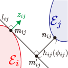
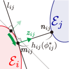
In this section, we formulate a novel CBF that ensures the forward invariance of the set in (4), namely preventing agent from colliding with agent . As mentioned previously and from [21, 22], it is difficult to derive the analytical solution of the distance between two ellipses, namely , in a form simple enough to be employed as a CBF. Furthermore, numerical solutions of cannot be employed as a CBF. To mitigate the difficulties, we design a novel CBF that incorporates a signed distance from a supporting line of agent to agent , depicted as in Fig. 2. Because could take a shorter length than with naive choices of the supporting line, we propose the procedure that drives to based on the gradient of an optimization problem.
III-A Separation Conditions for Two Elliptical Agents
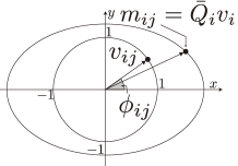
We first introduce a supporting line of agent , which contacts at the point , as depicted in Fig. 2. The point can be defined as
| (9) | ||||
| (10) |
with a positive definite matrix and a parameter . Here, the parameter is introduced to specify a point on the boundary of the ellipse , where the graphical interpretation is shown in Fig. 3. Then, the supporting line is described as
| (11) |
which is determined by and .
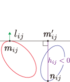
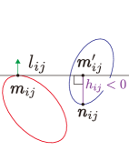
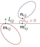
Let us derive the separation condition evaluated with the signed distance from the supporting line , which provides a positive value to a point in the different half-plane with , and a negative value otherwise as shown in Fig. 4. The point that minimizes the signed distance from the supporting line is determined by
| (12) |
Then, the minimum signed distance from is calculated by
| (13) |
which satisfies if and only if and are in the different half-plane separated by the line as shown in Fig. 4. In other words, if there exists that fulfills , then two ellipses are separated by the line . Note that is not the closest point to the supporting line as depicted in Fig. 4(a) and (b). In the remaining of this subsection, we analyze the property of assuming two agents and are fixed, hence denote as .
The fact that encodes the separation condition between two agents motivates us to employ as a CBF for ensuring collision avoidance between elliptical agents. However, the naive selection of the parameter , namely the line , could yield a shorter distance than the actual distance as depicted in Fig. 2(a). Because of this difference from , could overestimate the risk of collisions and hence cause too conservative evasive motion. To mitigate this gap, we propose the following optimization problem that intends to rotate the supporting line on the boundary of so that is maximized as
| (14a) | ||||
| s.t. | (14b) | |||
where its graphical interpretation is depicted in Fig. 2(b).
While, in the next subsection, we introduce the input to for maximizing , we first establish the connection between the optimization problem (14) and the actual distance between two agents, namely . For this goal, we introduce the following optimization problem, which optimal solution is equal to .
| (15a) | ||||
| s.t. | (15b) | |||
| (15c) | ||||
where signifies the condition . Then, the following theorem formalizes the relationship between and .
Theorem 1.
Proof.
The dual function of the problem (15) is
| (17) | |||
| (18) |
where , and are Lagrange multipliers. To simplify the first term in (18), we introduce , , and . Then, the first term is transformed as
| (19) |
Following the similar path to (19), the second term in (18) is expressed as
| (20) |
where and . Therefore, the dual problem can be expressed as follows:
| (21a) | ||||
| s.t. | (21b) | |||
In the case of , the gradient of is
| (23) |
Thus, the function has no extremum for all , and for it has the maximum value at . As a result, the following equation holds.
| (24) |
In the case of , the maximum value of is as follows:
| (25) |
Since (24) is equivalent to (25) if we substitute into (24), we can summarize them as
| (26) |
Considering that the second and fourth terms in (21a) are equal to and , respectively, we can simplify the problem (21) by utilizing (26) as follows:
| (27a) | ||||
| s.t. | (27b) | |||
| (27c) | ||||
Let us parameterize as
| (28) |
with so that the constraint (27b) is satisfied. Then, by substituting (28), and , the dual problem (27) can be transformed as follows
| (29a) | ||||
| s.t. | (29b) | |||
| (29c) | ||||
where the objective function (29a) can be described as . Notice that if ellipses and are separated, there always exists that satisfies . Considering the constraint (29c) and the fact is a variable independent of , we should set to maximize (29a). Therefore, by substituting to the problem (29), we obtain the optimization problem (14). This relation leads to the conclusion that the problem (14) is the dual of the optimization problem (15) if . Since the optimization problem (15) satisfies the Slater’s Condition [26, Sec. 5.2.3], the solution of (15) is equivalent to the solution of (14), which completes the proof. ∎
Theorem 1 implies that the proposed update law of the supporting line, described as the optimization problem (14) and Fig. 2, renders the actual distance between two ellipses. Furthermore, because of (16), the condition provides a sufficient condition for preventing collisions even if does not converge to the maximizer of (14). In the following subsection, we develop as a CBF together with presenting the update procedure of .
III-B CBFs Incorporating Rotating Supporting Lines
In this subsection, we first design the collision avoidance methods between two elliptical agents and , then extend the results to the case of agents. Hereafter, we regard as a function of , and as first defined in (13), though we have dropped the dependency of for notational convenience.
As mentioned in the previous subsection, we require a supporting line between agents and to evaluate the separation condition . Without loss of generality, we introduce a supporting line for the agent with a lower ID number. Then, as the supporting line is to be updated for maximizing , the model of the agent (2) now has to describe the dynamics of as well. Therefore, we introduce the augmented state to achieve collision avoidance between two agents and (), where the dynamics of the augmented state is
| (30) |
where .
As the nominal input for intending to maximize , we employ the following gradient-based input
| (31) |
The input (31) drives to a local maximum point, and hence preventing too conservative evasive motions caused by the difference between and . Note that the maximizer of changes as the agent and traverse. However, as is a virtual variable not dependent on the physical dynamics of the agents, we can make converge fast enough with large to follow the agent movement, as we will demonstrate in the simulations in Section IV-A.
Let us denote the nominal control input for the agent as , which is designed to achieve its own objective, e.g., reaching the goal position. Combining this nominal control input with (31), the nominal input for the augmented state is expressed as .
The goal of the collision avoidance strategy is to allow agents to execute their tasks encoded by while ensuring collision never occurs between agents. To achieve this objective, we propose the collision avoidance methods that render the following set forward invariant.
| (32) |
Since holds from Theorem 1, the set in (4) is also ensured to be forward invariant if we guarantee the forward invariance of . Similar to (8), this strategy can be achieved by derived from the following QP integrating as a CBF:
| (33a) | |||
| (33b) | |||
Note that the constraint (33b) is derived by calculating the Lie derivative of along and in (30).
As the proposed CBF prevents collision between elliptical agents and , we need to confirm whether there always exists the control input that satisfies (6) in the Definition 1 and it provides us the forward invariance property.
Theorem 2.
The function in (13) is a valid CBF when . Namely, for any , the following conditions hold.
| (34) | ||||
| (35) |
Proof.
and are given by
| (36) | ||||
| (37) |
Considering the fact and ,
holds. Therefore, the conditions and are always satisfied. ∎
Theorem 2 signifies there always exists the control input that renders the set forward invariant. Therefore, the collision is prevented if the state is in the safe set at the initial time. Note that if two ellipses do not collide with each other at the initial time, we can easily specify the initial that satisfies by any heuristic approach.
We then extend the collision avoidance method (33) to the scenario with agents. Similar to the case of the two agents, we need to introduce a supporting line for each pair of agents, resulting in numbers of CBFs for the whole system. Since the agent with a smaller ID in a pair owns a supporting line, a vector augmenting of agent is described as with . In addition, we introduce a vector combining as . Then, the ensemble state and CBFs of the system are expressed as and , respectively. With the introduced ensemble vectors, the collision avoidance method for agents can be achieved by derived from
| (38a) | ||||
| (38b) | ||||
where and since we assume a single integrator model.
IV Simulation Results
The proposed algorithm is implemented in simulations to verify that it guarantees collision avoidance between elliptical agents.
IV-A Simulation with Two Agents
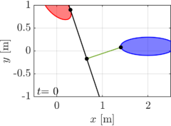
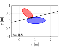
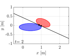
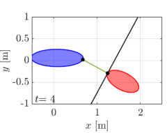
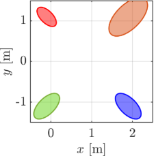
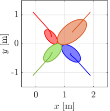
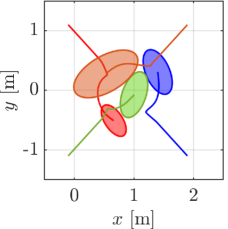
We first demonstrate our proposed algorithm with the two elliptical agents, the sizes of which are characterized by for a red agent and for a blue agent, respectively. The initial condition of the simulation is depicted in Fig. 5(a), with the initial pose , . Note that we randomly chose the initial from the range that yields a supporting line separating two ellipses. Two agents traverse the environment so that they intersect around the center of the field. We utilize for an extended class function in CBF conditions and for a nominal input to .
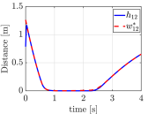
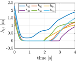
The snapshots of the simulations are presented in Fig. 5, which illustrate a supporting line incorporated in agent 1’s CBF as a black line. In addition, the distance between the supporting line and the blue ellipse is depicted as a green line. The snapshots demonstrate that the supporting line on agent is updated so that it separates two agents without causing any conservative transition in their evasive trajectories. The value of is illustrated in Fig. 6 together with the optimal solution of (15), namely the actual distance between two agents. Although and differ at the initial time since we set randomly, the proposed gradient-based input (31) successfully drives to the actual distance . Furthermore, Fig. 6 verifies that the input (31) rotates the supporting line so that follows the transition of the actual distance between two ellipses. We can also confirm that the value of keeps in the positive value, hence, collision avoidance is achieved.
IV-B Simulation with Four Agents
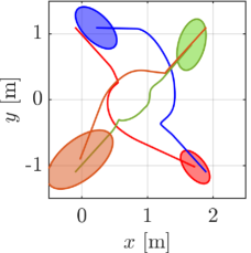
In the next simulation, we demonstrate our proposed algorithm with the four elliptical agents, the sizes of which are specified by for a red agent, for a blue agent, for a green agent and for an orange agent, respectively. The initial condition of the simulation is depicted in Fig. 7(a), with the initial pose , , and . All four agents traverse the environment so that they intersect around the center of the field. We utilize for an extended class function in CBF conditions and for a nominal input to each .
The snapshots of the simulation are presented in Fig. 7, where each agent is depicted with its trajectory. As illustrated in Fig. 7(b), all agents move straightly toward their goal positions until their distances become closer at the center. Then, the proposed methods modify the nominal input minimally invasive way so that the collision is avoided, as illustrated in Fig. 7(c) and (d). Note that the proposed CBF achieves the collision-free trajectories while changing the attitude of the agents in Fig. 7(c). Fig. 8 depicts the transitions of , where the proposed methods keep them in the positive value.
V Conclusion
In this paper, we proposed the collision avoidance method for elliptical agents that utilizes the novel CBF leveraging a supporting line between agents. We first introduced a supporting line of an agent to develop the separation condition of agents that is implementable as a CBF. However, we observed that a naive choice of a supporting line might render a shorter distance than the actual distance between two agents. To alleviate the conservativeness in this evaluation, we proposed the optimization problem that rotates the supporting line so that the distance between a supporting line and the other agent is maximized. We then proved that the maximum value derived from this optimization problem is equivalent to the actual distance between two agents. We presented the collision avoidance method incorporating the developed CBF together with the gradient ascent law for rotating the supporting line. Finally, numerical simulations showcased the validity of the proposed methods. Future works include extending the proposed framework to nonlinear systems through exponential CBF [27] while embracing 3D ellipsoidal agents.
VI Acknowledgement
We acknowledge Mr. Shunya Yamashita at Tokyo Institute of Technology for helpful discussions on the manuscript.
References
- [1] O. Arslan and D. E. Koditschek, “Voronoi-based coverage control of heterogeneous disk-shaped robots,” in Proc. IEEE Int. Conf. Robotics and Automation, 2016, pp. 4259–4266.
- [2] R. Funada, M. Santos, T. Gencho, J. Yamauchi, M. Fujita, and M. Egerstedt, “Visual coverage maintenance for quadcopters using nonsmooth barrier functions,” in Proc. IEEE Int. Conf. Robotics and Automation, 2020, pp. 3255–3261.
- [3] T. Miyano, J. Romberg, and M. Egerstedt, “Primal-dual gradient dynamics for cooperative unknown payload manipulation without communication,” in Proc. American Control Conf., 2020, pp. 2061–2067.
- [4] G.-B. Dai and Y.-C. Liu, “Distributed coordination and cooperation control for networked mobile manipulators,” IEEE Trans. Industrial Electronics, vol. 64, no. 6, pp. 5065–5074, 2017.
- [5] F. S. Barbosa, L. Lindemann, D. V. Dimarogonas, and J. Tumova, “Provably safe control of Lagrangian systems in obstacle-scattered environments,” in Proc. IEEE Conf. Decision and Control, 2020, pp. 2056–2061.
- [6] C. Zhang and J. M. Kovacs, “The application of small unmanned aerial systems for precision agriculture: A review,” Precision Agriculture, vol. 13, pp. 693–712, 2012.
- [7] Y. Rizk, M. Awad, and E. W. Tunstel, “Cooperative heterogeneous multi-robot systems: A survey,” ACM Comput. Surv., vol. 52, no. 2, 2019.
- [8] M. Hoy, A. S. Matveev, and A. V. Savkin, “Algorithms for collision-free navigation of mobile robots in complex cluttered environments: A survey,” Robotica, vol. 33, no. 3, pp. 463–497, 2015.
- [9] A. D. Ames, S. Coogan, M. Egerstedt, G. Notomista, K. Sreenath, and P. Tabuada, “Control barrier functions: Theory and applications,” in Proc. European Control Conf., 2019, pp. 3420–3431.
- [10] O. Khatib, “Real-time obstacle avoidance for manipulators and mobile robots,” in Autonomous Robot Vehicles. ”New York, NY: Springer New York, 1986, pp. 396–404.
- [11] D. V. Dimarogonas and K. H. Johansson, “On the stability of distance-based formation control,” in Proc. IEEE Conf. Decision and Control, 2008, pp. 1200–1205.
- [12] R. Olfati-Saber, “Flocking for multi-agent dynamic systems: Algorithms and theory,” IEEE Trans. Automatic Control, vol. 51, no. 3, pp. 401–420, 2006.
- [13] V. Gazi and K. M. Passino, “A class of attractions/repulsion functions for stable swarm aggregations,” Int. J. Control, vol. 77, no. 18, pp. 1567–1579, 2004.
- [14] D. M. Stipanović, P. F. Hokayem, M. W. Spong, and D. D. Šiljak, “Cooperative avoidance control for multiagent systems,” J. Dynamic Syst., Measurement, and Control, vol. 129, no. 5, pp. 699–707, 2007.
- [15] A. D. Ames, X. Xu, J. W. Grizzle, and P. Tabuada, “Control barrier function based quadratic programs for safety critical systems,” IEEE Trans. Automatic Control, vol. 62, no. 8, pp. 3861–3876, 2017.
- [16] L. Wang, A. D. Ames, and M. Egerstedt, “Safety barrier certificates for collisions-free multirobot systems,” IEEE Trans. Robotics, vol. 33, no. 3, pp. 661–674, 2017.
- [17] P. Glotfelter, I. Buckley, and M. Egerstedt, “Hybrid nonsmooth barrier functions with applications to provably safe and composable collision avoidance for robotic systems,” IEEE Robotics and Automation Letters, vol. 4, no. 2, pp. 1303–1310, 2019.
- [18] A. Singletary, K. Klingebiel, J. Bourne, A. Browning, P. Tokumaru, and A. Ames, “Comparative analysis of control barrier functions and artificial potential fields for obstacle avoidance,” in Proc. IEEE/RSJ Int. Conf. Intelligent Robots and Syst., 2021, pp. 8129–8136.
- [19] P. Glotfelter, J. Cortés, and M. Egerstedt, “A nonsmooth approach to controller synthesis for boolean specifications,” IEEE Trans. Automatic Control, vol. 66, no. 11, pp. 5160–5174, 2021.
- [20] G. Notomista and M. Egerstedt, “Persistification of robotic tasks,” IEEE Trans. Control Syst. Technol., vol. 29, no. 2, pp. 756–767, 2021.
- [21] K. D. Do, “Flocking for multiple ellipsoidal agents with limited communication ranges,” Int. Scholarly Research Notices, vol. 2013, p. 13, 2013.
- [22] C. K. Verginis and D. V. Dimarogonas, “Closed-form barrier functions for multi-agent ellipsoidal systems with uncertain Lagrangian dynamics,” IEEE Control Syst. Letters, vol. 3, no. 3, pp. 727–732, 2019.
- [23] M. Srinivasan, M. Abate, G. Nilsson, and S. Coogan, “Extent-compatible control barrier functions,” Syst. Control Letters, vol. 150, p. 104895, 2021.
- [24] W. Wang, J. Wang, and M.-S. Kim, “An algebraic condition for the separation of two ellipsoids,” Computer Aided Geometric Design, vol. 18, no. 6, pp. 531–539, 2001.
- [25] M. G. Choi, “Computing the closest approach distance of two ellipsoids,” Symmetry, vol. 12, no. 8, p. 1302, 2020.
- [26] S. Boyd and L. Vandenberghe, Convex Optimization. Cambridge University Press, 2004.
- [27] Q. Nguyen and K. Sreenath, “Exponential control barrier functions for enforcing high relative-degree safety-critical constraints,” in Proc. American Control Conf., 2016, pp. 322–328.