Coloring the Black Box:
What Synesthesia Tells Us about Character Embeddings
Abstract
In contrast to their word- or sentence-level counterparts, character embeddings are still poorly understood. We aim at closing this gap with an in-depth study of English character embeddings. For this, we use resources from research on grapheme–color synesthesia – a neuropsychological phenomenon where letters are associated with colors –, which give us insight into which characters are similar for synesthetes and how characters are organized in color space. Comparing 10 different character embeddings, we ask: How similar are character embeddings to a synesthete’s perception of characters? And how similar are character embeddings extracted from different models? We find that LSTMs agree with humans more than transformers. Comparing across tasks, grapheme-to-phoneme conversion results in the most human-like character embeddings. Finally, ELMo embeddings differ from both humans and other models.
1 Introduction
Neural network models have become crucial tools in natural language processing (NLP) and define the state of the art on a large variety of tasks Wang et al. (2018). However, they are difficult to understand and are often considered ”black boxes”.111This fact has led to the establishment of a workshop with the same name: https://blackboxnlp.github.io This can make their use difficult to defend in many settings, for instance in a legal context, and constitutes a barrier for model improvement. Therefore, a lot of research has been dedicated to investigating the information encoded by neural networks. Especially word embeddings, contextualized word representations, and language representation models like BERT Devlin et al. (2019) have been exhaustively studied Rogers et al. (2020).
Character embeddings are used for a large set of tasks, either as a supplement to word-level input, e.g., for part-of-speech tagging by Plank et al. (2016), or on their own, e.g., for character-level sequence-to-sequence (seq2seq) tasks by Kann and Schütze (2016). Despite this, they have not yet been explicitly analysed. One reason for this might be that identifying relevant properties to study is more challenging than for their word-level counterparts. However, we argue that, in order to truly shine light into black-box NLP models, it is necessary to understand each and every component of them.

In this paper, we perform a detailed study of English character embeddings. Our first contribution is a character similarity task (§3) in analogy to the word-based version: Do embeddings agree with humans on which pairs of characters are similar? While e.g., cat and tiger are generally considered more similar than cat and chair, this is not trivial for characters. For our annotations, we exploit a phenomenon called synesthesia. People with synesthesia, synesthetes, share perceptual experiences between two or more senses (§2). For grapheme–color synesthetes, each letter is associated with a color, which is consistent over a person’s life time Eagleman et al. (2007), cf. Figure 1. Using a dataset of letters from the English alphabet and the associated colors from 4269 synesthetes (Witthoft et al., 2015), we compute differences in color space (§3.3) as a proxy for character similarity.
As our second contribution, we propose a set of methods to characterize the structure of character embedding matrices (§4). The methods we propose are (i) a clustering analysis, (ii) computing the clustering coefficient, (iii) measuring betweenness centrality, and (iv) computing cut-distances.
Our final contribution is a detailed character embedding analysis (§6). We explore 6 types of embeddings, obtained from 4 different architectures trained on 3 different tasks, as well as 4 embedding matrices from pretrained ELMo models Peters et al. (2018). Comparing across models trained on the same task, character embeddings from LSTMs, which, similar to humans, process input sequentially, correlate more with human similarity scores than embeddings from transformers. Comparing across tasks, character embeddings from language modeling show a surprisingly low correlation with human judgments. In contrast, the correlation is highest for grapheme-to-phoneme conversion (G2P). This is in line with findings that colors perceived by synesthetes are influenced by the sound of each letter Asano and Yokosawa (2013).
2 Synesthesia
Synesthesia is the perceptual phenomenon that two or more sensory or cognitive pathways are co-activated in the brain by stimulating only one of them. For example, for a person with chromesthesia, a common form of synesthesia, hearing a particular sound evokes the visual perception of colors Cytowic (2018); Simner (2012).
By far the most common form of synesthesia is grapheme-color synesthesia, for which subjects report the perception of colors when seeing numerals or letters (cf. Figure 1). The neural basis behind the phenomenon is still a much debated topic, but evidence suggests it might be the result of increased effective connectivity between the brain areas involved Ramachandran and Hubbard (2001a). For example, visual area V4a in the ventral pathway, often associated with contextual processing and perception of color, has shown to be part of a complex in the fusiform gyrus exhibiting higher cortical thickness, volume, and surface area in synesthetes Hubbard et al. (2005). Belonging to this complex and adjacent to the color processing region is the area dedicated to the visual recognition and processing of graphemes, suggesting that a prominence of this type of synesthesia is due to higher region interconnectivity being more probable.
Additional evidence supports the idea that synesthetic associations often involve the extraction of meaning from a stimulus, suggesting that abstract constructions play a major role in the associations formed Mroczko-Wasowicz and Nikolic (2014). For cases where language is involved, semantics may in part underlie color representations of words and graphemes in V4.
3 A Character Similarity Task
3.1 Motivation: Word Similarity
Our first contribution is a character-level analogue of the word similarity task, an intrinsic evaluation method for word embeddings. It consists of judging the similarity of pairs of words, e.g., of cat and tiger. To obtain a gold standard for this task, human annotators assign similarity scores to a list of word pairs. This is not always trivial: are cat and bird more or less similar than cat and fish? However, people tend to agree on general tendencies.
Word embeddings are evaluated on similarity datasets as follows: The similarity – usually cosine similarity – of all pairs of words is computed. The agreement between models and human annotations is then quantified as the correlation between the two vectors of scores. Word embeddings with a higher performance on word similarity tasks are expected to perform better on downstream tasks, since they encode valuable information about words and the relationships between them.
3.2 From Word to Character Similarity
In order to design a character similarity task, we require a gold standard. However, we are not likely to get a meaningful answer when asking people if B and J are more similar than C and Q.
We solve this problem by looking at how different characters are represented by grapheme–color synesthetes in color space. This tells us how similar characters are perceived to be without having to ask explicitly. We leverage a dataset collected by Witthoft et al. (2015), which consists of letter-to-color mappings collected from 4269 synesthetes and compute pair-wise perceptually uniform distances between characters. Analogously to the word-level version of the task, we then take as our gold standard the average over all annotators. For embeddings, we compute cosine similarities between character vectors.
We differ from the word similarity task in an important detail: we do not evaluate the quality of embeddings. Instead, we aim to understand character embeddings by assessing how similar to the human perception of characters they are. In particular, we do not necessarily expect embeddings which score higher on our task to perform better on downstream applications.
3.3 Human Perception of Color Differences
To motivate the distance metric we use, we first summarize human perception of color. The visual process of color perception starts in the retina, where three types of light-sensitive receptors are tuned to respond broadly around three distinct frequencies in the visible spectrum. However, color perception is not simply reduced to combinations of these physiological responses. The human brain can perceive the same physical light frequency as a different color depending on a plethora of contextual markers, mostly due to further processing upstream of the retina into high-level visual cortical areas, where associations are formed between environmental cues and the object being visualized.
Important contextual properties of color affecting perception, often discussed in color theory as the Munsell (or HSL) color system, are its hue, saturation, and lightness. Combinations of these properties are interpreted in a highly non-linear manner by cortical areas tasked with color perception. Not surprisingly, simple metrics for color comparison, such as the Euclidean distance in RGB space, perform poorly in situations involving a color discrimination task. Constructing perceptually uniform metrics that deal with these perceived non-linearities is an active field of research. One standard metric for perceptual color comparison is the CIEDE2000 color difference Sharma et al. (2005), which includes several correction factors for a modified Euclidean metric on HSL space. We employ CIEDE2000 in our analysis.
4 Analysis of the Distance Matrix
CIEDE2000 allows us to obtain pair-wise distances between all letters in the alphabet by computing color differences for the associated colors as perceived by synesthetes. The character similarity task then compares vectors of pair-wise distances. However, we can gain additional insight from the distance matrices, which represent fully connected networks whose nodes are the letters in the alphabet and whose edges are weighted by the pair-wise differences. Thus, we further propose four well-established methods from network theory Newman (2018) for the analysis of character embeddings and human difference matrices.
Clustering analysis. To characterize the global structure of the network, we first propose Ward’s variance minimization algorithm to identify clusters, i.e., groups of letters that are similar to each other, but far away from other letters. Ward’s algorithm is part of a family of hierarchical clustering algorithms whose objective function aims at minimizing the variance within clusters Ward (1963). Starting from a forest of clusters (initially single nodes), the algorithm evaluates the Ward distance between a new cluster made up of clusters and , and a third cluster not used yet, as
| (1) |
with
| (2) | ||||
| (3) | ||||
| (4) |
where , and is the size of the cluster. If is a good cluster, then and are removed from the forest and the algorithm continues until only one cluster is left. Finally, the number of clusters, their sizes, and the Ward distances between clusters characterize the global structure of the network.
Clustering coefficient. The clustering coefficient provides a way to measure the degree to which nodes in a network cluster together. For a binary network, the local version represents the fraction of the number of pairs of neighbors of a node that are connected, over the total number of pairs of neighbors of said node, and it measures the influence of a node on its immediate neighbors. Several generalizations for weighted networks have been proposed Saramäki et al. (2007). Here, we use the average of the weights for neighbors in the subgraph of a node
where denotes weight normalized by the maximum weight in the network, and is the degree of the node (the sum of its edges’ weights). The average over all nodes is used as a proxy for the overall level of clustering within the network.
Betweenness centrality. Different concepts of centrality attempt to capture the relative importance of particular nodes in the network. One such concept, betweenness, measures the extent to which a node lies on the shortest path between pairs of nodes Brandes (2008). In a sense, it generalizes the clustering coefficient from a measure of the local influence of a node to immediate neighbors to the whole network. In particular, it accounts for nodes that connect two different clusters while not being a part of either. Betweenness centrality is computed as the fraction of all-pairs shortest paths that pass through a particular node
where the sum is over all nodes and in the network, and counts the number of shortest paths between two nodes, optionally taking into account if it passes through .
Cut-distance.
The fourth and last approach we propose to characterize our matrices of character distances is to employ a matrix norm called cut-norm. It is widely used in graph and network theory and has been shown to capture global features such as clustering and sparseness Frieze and Kannan (1999). The cut-norm of a matrix is defined as
i.e., the maximum over all possibles sub-matrix arrangements is taken as the norm. In practice, we compute it using an efficient implementation222https://pypi.org/project/cutnorm/ that relies on Grothendieck’s inequality for an approximation Alon and Naor (2004); Wen et al. (2013). In addition, the norm naturally gives rise to a distance metric that allows us to compare pairs of distance matrices directly.
5 Models and Tasks
We now describe the tasks and model architectures we employ to train different character embeddings.
5.1 Tasks
Language modeling. The task of language modeling consists of computing a probability distribution over all elements in a predefined vocabulary, given a sequence of past elements. Language models can either be used to assign a probability to an input sequence or to generate text by sampling from the probability distributions. We train language models on the character level, i.e., the vocabulary consists of the English alphabet.
All our language models are trained on wikitext-103.333https://s3.amazonaws.com/research.metamind.io/wikitext/wikitext-103-v1.zip We use the provided training, development, and test splits. The training set consists of roughly 1 million tokens.
Morphological inflection. In languages that exhibit rich inflectional morphology, words inflect: grammatical information like number, case, and tense are incorporated into the word itself. For instance, wrote is the inflected form of the English lemma write, expressing past tense.
The task of morphological inflection consists of mapping a lemma to an inflected form which is defined by a set of morphological tags. Morphological inflection is typically being cast as a character-level seq2seq task, where the characters of the lemma together with the morphological tags are the input, and the characters of the inflection are the output Kann and Schütze (2016):
We train our inflection models on the English training examples provided by Cotterell et al. (2017) and use the corresponding development and test sets with examples each.
Grapheme-to-phoneme conversion. Given a word’s spelling, G2P consists of generating an (IPA-like) representation of its pronunciation:
It has been shown that similar-sounding letters tend to be associated with similar synesthetic colors Asano and Yokosawa (2013). Hence, we assume that the embedding space induced by this task could be similar to human perception of characters.
We train all G2P models on examples extracted from the CMU Pronouncing Dictionary.444http://www.speech.cs.cmu.edu/cgi-bin/cmudict Our training, development, and test sets consist of 114,399, 5447, and 12,855 examples, respectively.555We use the splits provided at https://github.com/microsoft/CNTK/tree/master/Examples/SequenceToSequence/CMUDict/Data.
5.2 Architectures
To isolate the effects of task and model architecture, we train different architectures for each task. All test set performances are shown in Table 1. We train 50 models with different random seeds for seq2seq tasks, and 10 instances for language models. For our analysis, we look at the input embeddings and average pair-wise distances over models for each group. All models have been trained on an NVidia Tesla K80 GPU.
LSTM seq2seq architecture. Our first architecture is a seq2seq model similar to that by Bahdanau et al. (2015). It consists of a bi-directional long short-term memory (LSTM; Hochreiter and Schmidhuber, 1997) encoder and an LSTM decoder, which are connected via an attention mechanism. We apply it on the character level.
We train this architecture on morphological inflection () and G2P (), using the fairseq sequence modeling toolkit for our implementation.666https://github.com/pytorch/fairseq All embeddings and hidden states are 100-dimensional, and both encoder and decoder have 1 hidden layer. For training, we use an Adam optimizer Kingma and Ba (2014) with an initial learning rate of 0.001, dropout with a coefficient of , and a batch size of 20. To account for different training set sizes, we train our model for G2P for 15 and our model for inflection for 100 epochs.
Transformer seq2seq architecture. We further experiment with a transformer seq2seq architecture Vaswani et al. (2017). Similar to the LSTM seq2seq model, this architecture consists of an encoder and a decoder which are connected by an attention mechanism. However, the encoder and the decoder consist of combinations of feed-forward and attention layers instead of LSTMs.
We apply this architecture to morphological inflection () and G2P (), and implement the models using the fairseq toolkit. All embeddings have 256 dimensions, and hidden layers are 1024-dimensional. Both encoder and decoder have 4 layers, and use 4 attention heads. We employ an Adam optimizer with an initial learning rate of 0.001 for training, together with dropout with a coefficient of , and a batch size of 400. We train our models for G2P for 30 epochs and our models for morphological inflection for 100 epochs.
LSTM language model architecture. We also experiment with an LSTM language model (). This architecture consists of a unidirectional LSTM, and it receives the last generated character as input at each time step.
Our implementation is based on the official pytorch LSTM language model example.777https://github.com/pytorch/examples/tree/master/word_language_model We use the default hyperparameters except for the following: our embeddings and LSTM hidden states are 512-dimensional, we use 2 hidden layers, and we train for 2 epochs with a batch size of 64.
Transformer language model architecture. Our last architecture is a transformer language model (). Like the LSTM language model, it receives previously generated characters as input and computes a probability distribution over the character vocabulary.
Again, we use the fairseq toolkit for our implementation, and employ the default hyperparameters for the transformer language model. We use an Adam optimizer with an initial learning rate of 0.0005 for training, and dropout with a coefficient of 0.1. This model is trained for 3 epochs.
| 0.95 | 0.94 | 0.64 | 0.62 | 3.37 | 2.62 |
| 50 | 50 | 50 | 50 | 10 | 10 |
5.3 Pretrained Models
We further analyze the character embeddings of ELMo models Peters et al. (2018). ELMo models are pretrained networks, aimed at producing contextualized word embeddings for use in downstream NLP tasks. The model architecture consists of a convolutional layer over character embeddings, whose output is then fed into a 2-layer bidirectional LSTM. ELMo models are trained with a bidirectional language modeling objective.
We experiment with 4 English models which are available online:888https://allennlp.org/elmo small (), medium (), original () and original-5.5B (). Those models differ in the number of their parameters and the amount of text they have been trained on: and have 13.6 million and 28 million parameters, respectively. Both and have 93.6 million parameters. All models except for have been trained on the 1 Billion Word Benchmark.999http://www.statmt.org/lm-benchmark/ has been trained on a combination of Wikipedia and news crawl data, which together result in a dataset of 5.5 billion tokens.
6 Character Embedding Analysis
6.1 Results on the Character Similarity Task

The Pearson correlation of all models with human judgements as well as with each other is shown in Figure 2. shows the highest correlation with 0.30, while is not correlated at all, and obtains the strongest negative correlation with .
More generally, we see that most models are correlated with each other (between and ), with the exception of the ELMos: the predictions of are the only ones which have a Pearson correlation with those of some other models.
Comparing to human scores, we find the following patterns: embeddings from seq2seq tasks show a higher correlation than embeddings from language models. Even ELMo models, which are trained on large amounts of text, obtain a maximum correlation of . Thus, we conclude that language modeling does not result in embeddings which perform well on our character similarity task. Embeddings for G2P correlate more strongly with human character perception than embeddings from inflection, when comparing identical architectures. This is noteworthy, since colors perceived by synesthetes are supposed to be influenced by the sound of each letter Asano and Yokosawa (2013), similar to the embeddings for G2P. Finally, comparing across architectures, we see that LSTM models correlate stronger with human judgments than transformer models, which is in line with the common understanding that recurrent neural networks might be better models of human cognition.

6.2 Comparing Humans and Machines
Clustering analysis. First, we look at the global structure of all character embeddings (cf. Figure 5). All but the ELMo models exhibit a marked separation between a tight cluster of vowels (AEIOU) or extended vowels (+Y), which are highly similar, and the rest of the alphabet. In contrast, this distinction is not found for humans, neither for individuals nor the average distance matrix. Despite this, the human average does present a clear global structure (cf. appendix for details). One clear cluster is BDGJKMNPQRVWXZ, with the particularly close pairs MN and XZ, perhaps due to the letters’ shape, sound, or proximity in the alphabet. This cluster is far away from the letters in AES, which themselves do not form a cluster. Another cluster, on average far form the first, is formed by the letters CILOUY.
Apart from the clear separation between vowels and consonants, character embeddings exhibit rich additional structure (cf. Figure 5). For , the cluster BCFHJMPQW contains the tighter sub-cluster BJQW that is similar to the letters GKVX. In contrast, has the two small clusters HJKQ and LNR far from each other, and a less clear-cut structure among the rest of the consonants.
Embeddings from exhibit a structure clearly connected to the G2P task. The distance network has many small clusters of similar sounding letters, e.g., UW,IJ,JY,GJ,CKQ,SXZ, and BFPV. ’s counterpart, , produces similar groupings, but displays a more homogeneous structure overall.
has the tight cluster KSXYZ within the larger BCDFGKMPSTVWXYZ cluster, and weaker connections between other letters. has a clearer cluster structure, showing the strongest separation between vowels and consonants, especially from the non-cluster JKQXZ, which is also well-separated from other consonants. ELMo models are outliers in that they do not present a clear global structure: only loose clusters can be identified.
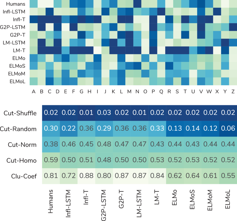
Cluster coefficient. Looking at the cluster coefficients (cf. Figure 4, last row) we also see a difference between ELMo embeddings and the other models: all models except for the ELMos have cluster coefficients between 0.72 and 0.88 and, thus, close to the human average of 0.81. In contrast, the cluster coefficients for ELMo embeddings are between for and for .
Betweenness centrality. The local values of betweenness centrality (cf. Figure 4) show the rich structure of the similarity matrices for most embeddings. For all but the ELMo models, the majority of letters have either extremely high or low levels of betweenness. In particular vowels tend to occupy prominent places in the network structure. Humans, in contrast, are more similar to ELMo embeddings.
Cut-distance. Looking at cut-distances (cf. Figure 4), we find that the structure of ELMo embeddings is significantly more similar to a random matrix than that of the other embeddings. The cut-distances (cf. Figure 3) between humans and embeddings largely agree with the conclusions from Section 6.1 – and the ELMo models are respectively the most similar and dissimilar –, even though correlation for node-to-node similarities does not necessarily imply a similar global structure.

7 Related Work
Neural network analysis. A lot of ink has been spilled on what neural network models learn and how. For instance, Zhang and Bowman (2018) investigated different pretraining objectives on their ability to induce syntactic and part-of-speech information. Pruksachatkun et al. (2020) studied model performance on probing tasks to investigate what models learn from intermediate-task training. Belinkov et al. (2017) explored what neural machine translation models learn about morphology.
Other work created test sets to evaluate specific linguistic model abilities. Linzen et al. (2016) made a dataset to investigate the ability of neural networks to detect mismatches in subject–verb agreement in the presence of distractor nouns. Warstadt et al. (2019) created a benchmark called BLiMP to assess the ability of language models to handle specific syntactic phenomena in English. Mueller et al. (2020) introduced a similar suite of test sets in English, French, German, Hebrew and Russian, also focusing on syntactic phenomena. Similarly, Xiang et al. (2021) presented CLiMP, a benchmark for the evaluation of Chinese language models.
Besides that, attention mechanisms Bahdanau et al. (2015) in neural models have been common subjects of investigation. Jain and Wallace (2019) claimed that ”attention is not explanation”, to be later on challenged by Wiegreffe and Pinter (2019), who argued that ”attention is not not explanation”. However, the relationship between inputs, attention weights, and outputs is still poorly understood.
Furthermore, our work is related to research on which information is learned and how information is encoded by so-called language representation models, e.g., BERT Devlin et al. (2019) or RoBERTa Liu et al. (2019). Similar to attention in other models, attention in BERT has been investigated exhaustively. Clark et al. (2019) found that it captures substantial syntactic information, and Vig (2019) built a visualization tool for the attention mechanism. Hewitt and Manning (2019) evaluated whether syntax trees could be recovered from BERT or ELMo’s word representation space. An overview of over 40 different studies of BERT can be found in Rogers et al. (2020).
Embedding analysis. The research which is closest to our work investigates which information is captured by different types of embeddings, often by training a classifier to predict certain features of interest. For instance, Kann et al. (2019) used a classifier-based approach to examine whether word and sentence embeddings encode information about the frame-selectional properties of verbs. Ettinger et al. (2016) investigated the grammatical information contained in sentence embeddings regarding multiple linguistic phenomena. Qian et al. (2016) mapped a dense embedding to a sparse linguistic property space to explore the contained information. Bjerva and Augenstein (2018) studied language embeddings.
Different word similarity datasets have been used for word embedding evaluation, for instance RG-65 Rubenstein and Goodenough (1965), WordSim-353 Finkelstein et al. (2002), or SimLex-999 Hill et al. (2015).
In contrast to the work in this paragraph, which was concerned with word or sentence embeddings, we aim at understanding character embeddings.
8 Conclusion
In this paper, we performed an in-depth analysis of character embeddings extracted from various character-level models for NLP. We leveraged resources from research on grapheme–color synesthesia – a neuropsychological phenomenon where letters are associated with colors –, to construct a dataset for a character similarity task. We further performed an analysis of networks representing characters as nodes and similarities as edge weights to understand how characters are organized by human synesthetes in comparison to character embeddings. Analysing 10 different character embeddings, we found that LSTMs agreed with humans more than transformer models. Comparing different tasks, G2P resulted in embeddings more similar to human character representions than inflection and, by a wide margin, language modeling. ELMo embeddings differed from humans and other models in that they exhibited no clear structure.
Acknowledgments
We would like to thank Manuel Mager and the anonymous reviewers for their feedback on this work. Mauro M. Monsalve-Mercado acknowledges financial support from the Center for Theoretical Neuroscience at Columbia University through the NSF NeuroNex Award DBI-1707398 and The Gatsby Charitable Foundation.
References
- Alon and Naor (2004) Noga Alon and Assaf Naor. 2004. Approximating the cut-norm via grothendieck’s inequality. In Proceedings of the Thirty-Sixth Annual ACM Symposium on Theory of Computing, STOC ’04, page 72–80, New York, NY, USA. Association for Computing Machinery.
- Asano and Yokosawa (2013) Michiko Asano and Kazuhiko Yokosawa. 2013. Grapheme learning and grapheme-color synesthesia: toward a comprehensive model of grapheme-color association. Frontiers in human neuroscience, 7:757.
- Bahdanau et al. (2015) Dzmitry Bahdanau, Kyunghyun Cho, and Yoshua Bengio. 2015. Neural machine translation by jointly learning to align and translate. In ICLR.
- Belinkov et al. (2017) Yonatan Belinkov, Nadir Durrani, Fahim Dalvi, Hassan Sajjad, and James Glass. 2017. What do neural machine translation models learn about morphology? In Proceedings of the 55th Annual Meeting of the Association for Computational Linguistics (Volume 1: Long Papers), pages 861–872, Vancouver, Canada. Association for Computational Linguistics.
- Bjerva and Augenstein (2018) Johannes Bjerva and Isabelle Augenstein. 2018. From phonology to syntax: Unsupervised linguistic typology at different levels with language embeddings. In Proceedings of the 2018 Conference of the North American Chapter of the Association for Computational Linguistics: Human Language Technologies, Volume 1 (Long Papers), pages 907–916, New Orleans, Louisiana. Association for Computational Linguistics.
- Brandes (2008) Ulrik Brandes. 2008. On variants of shortest-path betweenness centrality and their generic computation. Social Networks, 30(2):136 – 145.
- Clark et al. (2019) Kevin Clark, Urvashi Khandelwal, Omer Levy, and Christopher D Manning. 2019. What does BERT look at? An analysis of BERT’s attention. arXiv preprint arXiv:1906.04341.
- Cotterell et al. (2017) Ryan Cotterell, Christo Kirov, John Sylak-Glassman, Géraldine Walther, Ekaterina Vylomova, Patrick Xia, Manaal Faruqui, Sandra Kübler, David Yarowsky, Jason Eisner, and Mans Hulden. 2017. CoNLL-SIGMORPHON 2017 shared task: Universal morphological reinflection in 52 languages. In Proceedings of the CoNLL SIGMORPHON 2017 Shared Task: Universal Morphological Reinflection, pages 1–30, Vancouver. Association for Computational Linguistics.
- Cytowic (2018) R.E. Cytowic. 2018. Synesthesia. MIT Press Essential Knowledge series. MIT Press.
- Devlin et al. (2019) Jacob Devlin, Ming-Wei Chang, Kenton Lee, and Kristina Toutanova. 2019. BERT: Pre-training of deep bidirectional transformers for language understanding. In Proceedings of the 2019 Conference of the North American Chapter of the Association for Computational Linguistics: Human Language Technologies, Volume 1 (Long and Short Papers), pages 4171–4186, Minneapolis, Minnesota. Association for Computational Linguistics.
- Eagleman et al. (2007) David M Eagleman, Arielle D Kagan, Stephanie S Nelson, Deepak Sagaram, and Anand K Sarma. 2007. A standardized test battery for the study of synesthesia. Journal of neuroscience methods, 159(1):139–145.
- Ettinger et al. (2016) Allyson Ettinger, Ahmed Elgohary, and Philip Resnik. 2016. Probing for semantic evidence of composition by means of simple classification tasks. In Proceedings of the 1st Workshop on Evaluating Vector-Space Representations for NLP, pages 134–139, Berlin, Germany. Association for Computational Linguistics.
- Finkelstein et al. (2002) Lev Finkelstein, Evgeniy Gabrilovich, Yossi Matias, Ehud Rivlin, Zach Solan, Gadi Wolfman, and Eytan Ruppin. 2002. Placing search in context: The concept revisited. ACM Trans. Inf. Syst., 20(1):116–131.
- Frieze and Kannan (1999) Alan Frieze and Ravindran Kannan. 1999. Quick approximation to matrices and applications. Combinatorica, 19:175–220.
- Hewitt and Manning (2019) John Hewitt and Christopher D. Manning. 2019. A structural probe for finding syntax in word representations. In Proceedings of the 2019 Conference of the North American Chapter of the Association for Computational Linguistics: Human Language Technologies, Volume 1 (Long and Short Papers), pages 4129–4138, Minneapolis, Minnesota. Association for Computational Linguistics.
- Hill et al. (2015) Felix Hill, Roi Reichart, and Anna Korhonen. 2015. SimLex-999: Evaluating semantic models with (genuine) similarity estimation. Computational Linguistics, 41(4):665–695.
- Hochreiter and Schmidhuber (1997) Sepp Hochreiter and Jürgen Schmidhuber. 1997. Long short-term memory. Neural computation, 9(8):1735–1780.
- Hubbard et al. (2005) Edward M. Hubbard, A. Cyrus Arman, Vilayanur S. Ramachandran, and Geoffrey M. Boynton. 2005. Individual differences among grapheme-color synesthetes: Brain-behavior correlations. Neuron, 45(6):975 – 985.
- Jain and Wallace (2019) Sarthak Jain and Byron C. Wallace. 2019. Attention is not Explanation. In Proceedings of the 2019 Conference of the North American Chapter of the Association for Computational Linguistics: Human Language Technologies, Volume 1 (Long and Short Papers), pages 3543–3556, Minneapolis, Minnesota. Association for Computational Linguistics.
- Kann and Schütze (2016) Katharina Kann and Hinrich Schütze. 2016. Single-model encoder-decoder with explicit morphological representation for reinflection. In Proceedings of the 54th Annual Meeting of the Association for Computational Linguistics (Volume 2: Short Papers), pages 555–560, Berlin, Germany. Association for Computational Linguistics.
- Kann et al. (2019) Katharina Kann, Alex Warstadt, Adina Williams, and Samuel R. Bowman. 2019. Verb argument structure alternations in word and sentence embeddings. In Proceedings of the Society for Computation in Linguistics (SCiL) 2019, pages 287–297.
- Kingma and Ba (2014) Diederik P Kingma and Jimmy Ba. 2014. Adam: A method for stochastic optimization. arXiv preprint arXiv:1412.6980.
- Linzen et al. (2016) Tal Linzen, Emmanuel Dupoux, and Yoav Goldberg. 2016. Assessing the ability of LSTMs to learn syntax-sensitive dependencies. Transactions of the Association for Computational Linguistics, 4:521–535.
- Liu et al. (2019) Yinhan Liu, Myle Ott, Naman Goyal, Jingfei Du, Mandar Joshi, Danqi Chen, Omer Levy, Mike Lewis, Luke Zettlemoyer, and Veselin Stoyanov. 2019. Roberta: A robustly optimized bert pretraining approach. arXiv preprint arXiv:1907.11692.
- Mroczko-Wasowicz and Nikolic (2014) Aleksandra Mroczko-Wasowicz and Danko Nikolic. 2014. Semantic mechanisms may be responsible for developing synesthesia. Frontiers in Human Neuroscience, 8:509.
- Mueller et al. (2020) Aaron Mueller, Garrett Nicolai, Panayiota Petrou-Zeniou, Natalia Talmina, and Tal Linzen. 2020. Cross-linguistic syntactic evaluation of word prediction models. arXiv preprint arXiv:2005.00187.
- Newman (2018) M. Newman. 2018. Networks. OUP Oxford.
- Peters et al. (2018) Matthew Peters, Mark Neumann, Mohit Iyyer, Matt Gardner, Christopher Clark, Kenton Lee, and Luke Zettlemoyer. 2018. Deep contextualized word representations. In Proceedings of the 2018 Conference of the North American Chapter of the Association for Computational Linguistics: Human Language Technologies, Volume 1 (Long Papers), pages 2227–2237, New Orleans, Louisiana. Association for Computational Linguistics.
- Plank et al. (2016) Barbara Plank, Anders Søgaard, and Yoav Goldberg. 2016. Multilingual part-of-speech tagging with bidirectional long short-term memory models and auxiliary loss. In Proceedings of the 54th Annual Meeting of the Association for Computational Linguistics (Volume 2: Short Papers), pages 412–418, Berlin, Germany. Association for Computational Linguistics.
- Pruksachatkun et al. (2020) Yada Pruksachatkun, Jason Phang, Haokun Liu, Phu Mon Htut, Xiaoyi Zhang, Richard Yuanzhe Pang, Clara Vania, Katharina Kann, and Samuel R Bowman. 2020. Intermediate-task transfer learning with pretrained models for natural language understanding: Wen and why does it work? arXiv preprint arXiv:2005.00628.
- Qian et al. (2016) Peng Qian, Xipeng Qiu, and Xuanjing Huang. 2016. Investigating language universal and specific properties in word embeddings. In Proceedings of the 54th Annual Meeting of the Association for Computational Linguistics (Volume 1: Long Papers), pages 1478–1488, Berlin, Germany. Association for Computational Linguistics.
- Ramachandran and Hubbard (2001a) V. S. Ramachandran and E. M. Hubbard. 2001a. Psychophysical investigations into the neural basis of synaesthesia. Proceedings of the Royal Society of London. Series B: Biological Sciences, 268(1470):979–983.
- Ramachandran and Hubbard (2001b) V. S. Ramachandran and E. M. Hubbard. 2001b. Synaesthesia–a window into perception, thought and language. Journal of Consciousness Studies, 8(12):3–34.
- Rogers et al. (2020) Anna Rogers, Olga Kovaleva, and Anna Rumshisky. 2020. A primer in bertology: What we know about how BERT works. arXiv preprint arXiv:2002.12327.
- Rubenstein and Goodenough (1965) Herbert Rubenstein and John B. Goodenough. 1965. Contextual correlates of synonymy. Commun. ACM, 8(10):627–633.
- Saramäki et al. (2007) Jari Saramäki, Mikko Kivelä, Jukka-Pekka Onnela, Kimmo Kaski, and János Kertész. 2007. Generalizations of the clustering coefficient to weighted complex networks. Phys. Rev. E, 75:027105.
- Sharma et al. (2005) Gaurav Sharma, Wencheng Wu, and Edul N. Dalal. 2005. The ciede2000 color-difference formula: Implementation notes, supplementary test data, and mathematical observations. Color Research & Application, 30(1):21–30.
- Simner (2007) Julia Simner. 2007. Beyond perception: Synaesthesia as a psycholinguistic phenomenon. Trends in Cognitive Sciences, 11(1):23–29.
- Simner (2012) Julia Simner. 2012. Defining synaesthesia. British journal of psychology, 103(1):1–15.
- Vaswani et al. (2017) Ashish Vaswani, Noam Shazeer, Niki Parmar, Jakob Uszkoreit, Llion Jones, Aidan N Gomez, Łukasz Kaiser, and Illia Polosukhin. 2017. Attention is all you need. In NeurIPS.
- Vig (2019) Jesse Vig. 2019. Visualizing attention in transformer-based language representation models. arXiv preprint arXiv:1904.02679.
- Wang et al. (2018) Alex Wang, Amanpreet Singh, Julian Michael, Felix Hill, Omer Levy, and Samuel Bowman. 2018. GLUE: A multi-task benchmark and analysis platform for natural language understanding. In Proceedings of the 2018 EMNLP Workshop BlackboxNLP: Analyzing and Interpreting Neural Networks for NLP, pages 353–355, Brussels, Belgium. Association for Computational Linguistics.
- Ward (1963) Joe Ward. 1963. Hierarchical grouping to optimize an objective function. Journal of the American Statistical Association, 58(301):236–244.
- Warstadt et al. (2019) Alex Warstadt, Alicia Parrish, Haokun Liu, Anhad Mohananey, Wei Peng, Sheng-Fu Wang, and Samuel R Bowman. 2019. Blimp: A benchmark of linguistic minimal pairs for english. arXiv preprint arXiv:1912.00582.
- Wen et al. (2013) Miaomiao Wen, Zeyu Zheng, Hyeju Jang, Guang Xiang, and Carolyn Penstein Rosé. 2013. Extracting events with informal temporal references in personal histories in online communities. In Proceedings of the 51st Annual Meeting of the Association for Computational Linguistics (Volume 2: Short Papers), pages 836–842, Sofia, Bulgaria. Association for Computational Linguistics.
- Wiegreffe and Pinter (2019) Sarah Wiegreffe and Yuval Pinter. 2019. Attention is not not explanation. In Proceedings of the 2019 Conference on Empirical Methods in Natural Language Processing and the 9th International Joint Conference on Natural Language Processing (EMNLP-IJCNLP), pages 11–20, Hong Kong, China. Association for Computational Linguistics.
- Witthoft et al. (2015) Nathan Witthoft, Jonathan Winawer, and David M Eagleman. 2015. Prevalence of learned grapheme-color pairings in a large online sample of synesthetes. PLoS One, 10(3).
- Xiang et al. (2021) Beilei Xiang, Changbing Yang, Yu Li, Alex Warstadt, and Katharina Kann. 2021. CLiMP: A benchmark for Chinese language model evaluation. In Proceedings of the 16th Conference of the European Chapter of the Association for Computational Linguistics.
- Zhang and Bowman (2018) Kelly Zhang and Samuel Bowman. 2018. Language modeling teaches you more than translation does: Lessons learned through auxiliary syntactic task analysis. In Proceedings of the 2018 EMNLP Workshop BlackboxNLP: Analyzing and Interpreting Neural Networks for NLP, pages 359–361, Brussels, Belgium. Association for Computational Linguistics.
Appendix A: Statistics
| X–Z, M–N, R–X, K–X, H–N, M–R, O–U, M–W, V–Z, O–Q |
| B–Y, B–C, C–R, C–M, M–Y, R–Y, C–X, I–R, P–Y, C–Z |
Appendix B: Analysis of Color Differences of Characters as Perceived by Synesthetes
In additional to the most important findings mentioned in the main part of this paper, we further present an in-depth study of the character similarities according to human synesthetes in this section.
Clustering Analysis. For each individual, we compute a character difference matrix using CIEDI2000 (normalized to values between 0 and 1). We then use Ward’s hierarchical clustering algorithm to explore hidden structural features. Several examples suggest that individual synesthetes tend to represent certain groups of letters with closely matching colors, since their perceptual color differences tend to form tight clusters (Figure 6A), as opposed to the node-to-node average over the entire population of synesthetes (Figure 6B). To make this finding concrete, we compute several measures aimed to address the degree of clustering of each network.
First, we compute the distances between identified clusters in the distance matrix for each individual (Figure 6C). Pooled over the whole population, the distribution of cluster distances reveal an over-representation of small distances when compared to shuffled data. Over-represented small clustered distances and large jumps to big distances implies the existence of just a handful of tight clusters with small within-cluster distances and larger inter-cluster distances, as suggested by the dendrogram examples in Figure 6A.
Imposing a cut-off cluster distance for the dendrograms, we effectively select the cluster structure of the distance matrix. Although several methods for selecting the cut-off have been studied, they often strongly depend on the nature of the dataset in question. Using three largely different cut-offs we find robustly that each distance matrix encodes only a handful of tight clusters (cf. Figures 6D, E), typically around 3 to 5 clusters with an average size of 6 letters per cluster.
Clustering coefficient. Next, we compute the local clustering coefficient for each node in each distance matrix and observe no strong differences among nodes belonging to the same matrix. For each matrix, we average the cluster coefficient over all nodes and look at their distribution by pooling over all individuals (cf. Figure 6F). This reveals a narrow distribution of low clustering coefficients peaked around , implying a small average distance of any node to its neighbours. For comparison, we compute the clustering coefficient for a random uniform distance matrix (symmetric with zeroes in its diagonal) whose coefficient places at (averaged over 100 iterations), and also for a homogeneous distance matrix (all entries are equal with a zero diagonal) with a coefficient of . Moreover, we repeat the analysis for the node-to-node average distance matrix and show a relatively higher coefficient (), implying higher distances on average for any node with respect to its neighbors.
Betweenness centrality. Next, we examine the betweenness centrality of nodes (cf. Figure 6H). We compute this measure on the auxiliary similarity matrix , where is a distance matrix, in order to interpret high betweenness values as the most important nodes. The distribution over all individuals reveals the top-ranking nodes as CEILOSY. These are the nodes found to be in most shortest paths between pair of nodes, and possibly lie at the intersection between otherwise separate clusters.
Cut-distance. Finally, cut-distances between the individual distance matrices and a reference matrix offer an additional characterization of their global structure. We compute cut-distances with respect to a zero matrix (the cut-norm), a random and an homogeneous matrix (defined as in the last paragraph), and with respect to shuffled versions of themselves, averaged over 100 iterations (cf. Figure 6G). We find narrow distributions suggesting all individuals share a similar global structure.
