Combined Left and Right Temporal Robustness
for Control under STL Specifications
Abstract
Many modern autonomous systems, particularly multi-agent systems, are time-critical and need to be robust against timing uncertainties. Previous works have studied left and right time robustness of signal temporal logic specifications by considering time shifts in the predicates that are either only to the left or only to the right. We propose a combined notion of temporal robustness which simultaneously considers left and right time shifts. For instance, in a scenario where a robot plans a trajectory around a pedestrian, this combined notion can now capture uncertainty of the pedestrian arriving earlier or later than anticipated. We first derive desirable properties of this new notion with respect to left and right time shifts and then design control laws for linear systems that maximize temporal robustness using mixed-integer linear programming. Finally, we present two case studies to illustrate how the proposed temporal robustness accounts for timing uncertainties.
Keywords: time-critical systems, signal temporal logic, temporal robustness, control design, formal synthesis
I INTRODUCTION
This paper studies temporal robustness of time-critical systems, i.e., systems in which meeting real-time safety constraints is of great importance. Examples of time-critical systems include multi-robot systems and self-driving cars. While time-critical systems may satisfy their safety constraints under nominal operating conditions, already slight temporal perturbations such as time delays may jeopardize its safety if the system is not robust against such perturbations.
A common way to express real-time constraints is to use signal temporal logic (STL) [1]. Spatial robustness of STL specifications, quantifying permissible spatial perturbations, has been widely studied in the literature, see e.g., [2, 3, 4]. For control under spatial robustness objectives, there exist mixed-integer linear programming (MILP) approaches [5, 6, 7], gradient-descent searches [8, 9], control barrier functions for STL [10, 11], and learning-based frameworks [12]. However, these notions do not directly capture any robustness against temporal uncertainties. A first attempt to define time robustness for STL specifications was made in [13]. The authors define the left (right) time robustness by quantifying the maximal permissible left (right) time shifts in the predicates of the STL specification that do not result in a violation of the specification. In our previous works [14, 15], we analyze various properties of left (right) time robustness and propose an MILP encoding to control linear systems such that the left (right) time robustness is maximized. We continue along these lines and propose a novel notion of temporal robustness to account for both forward and backward temporal perturbations.
Besides the aforementioned notion of left (right) time robustness, there exist various other time robustness notions. Averaged STL was presented in [16] and captures temporal robustness by averaging spatial robustness over time intervals. Hybrid system conformance, see e.g., [17, 18], quantifies the closeness of hybrid systems trajectories and measures a combination of spatial and time robustness, but does not allow for asynchronous time shift in the predicates. The authors in [19] introduce a metric that can quantify the temporal relaxation of STL specifications. Tailored to multi-agent systems, the authors in [20, 21] propose counting linear temporal logic which requires a minimum number of agents for the satisfaction of a specification. The authors design control laws for such specifications where agents can implement their plans asynchronously, which can even account for time scaling effects, e.g., an agent pauses or speeds up, and not only time shifts in the predicate signal as we consider in this work. Temporal robustness of stochastic signals has been considered in [22] by using risk measures, but the authors there consider time shifts in the system signal, opposed to time shifts in predicates. In [23], monitoring of STL specifications under timing uncertainty in the underlying signal is considered by using over- and under-approximation of the satisfaction times of predicates. While [24] considers the time sensitive control for a subset of STL specifications, the authors in [25] present the time window temporal logic that is used in [26, 27] to obtain control laws for finding temporal relaxations when the specification is not satisfiable. In [28], the STL-based resiliency for cyber-physical system is presented that can capture temporal violations by recoverability and durability.
We make the following contributions. First, we propose a novel notion of temporal robustness for STL specifications to account for forward and backward temporal perturbations. We quantify the amount of permissible time shifts in the STL predicates to the left and right. We then show a set of desirable properties of our definition. Furthermore, we propose an MILP encoding for control of linear systems under the temporal robustness objective.
II Signal Temporal Logic (STL)
Let be a discrete-time signal with (we assume that includes ) being the time domain and being the state at time , where is a metric space. We call the set of all signals the signal space . A predicate is defined as , where is a real-valued function of the state . Let be a time interval. For any time point , we define the set . The syntax of Signal Temporal Logic (STL) is defined recursively as follows [1]:
| (1) |
where is a predicate from a set of predicates , and are the Boolean negation and conjunction, respectively, and is the Until temporal operator over a time interval . One can further define additional STL operators such as (disjunction), (eventually) and (always).
The semantics of an STL formula define when a signal satisfies at time . Commonly, it is given via the STL characteristic function , see [13] for details. Intuitively, when , it holds that the signal satisfies the formula at time , while indicates that does not satisfy at time .
While the semantics of STL indicate if the signal satisfies a given specification at time , the left and right time robustness measures how robustly a signal satisfies a given specification at time with respect to perturbations in time [13]. The left and right time robustness of a formula relative to a signal at time is defined recursively. For instance, the left and right time robustness of a predicate are defined as follows:
and then, to obtain the , one needs to apply the standard recursive / rules to each , similarly to the characteristic function , see [15] for details.
The sign of the left (right) time robustness reflects the satisfaction of the specification. Formally, if then and if then . In [15], we also showed that the absolute value of the left (right) time robustness measures how robustly a signal satisfies a formula at time with respect to time shifts in the predicates of formula . In fact, one can asynchronously shift predicates in time to the left by up to and the specification will not change its satisfaction. Formally, for , where is the number of predicates, if then , where and is a -early signal111The signal is called a -early signal if , , . The signal is called a -late signal if , , , see [15].. Analogously, if one shifts predicates in time to the right by up to then will not change its satisfaction. Formally, for , if then , where is a -late signal.
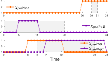
Example 1
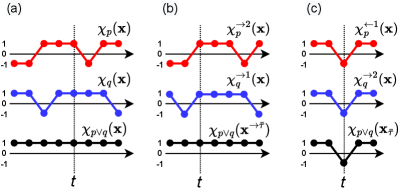
In Fig. 1(a), we plotted a characteristic function of two predicates and and the formula . The right time robustness is (since and ). Hence, the predicates can be shifted by up to time steps to the right and the formula at time must still be satisfied, see Fig. 1(b). The left time robustness is (since and ). The predicates can thus be shifted by up to time steps to the left and the formula must still be satisfied.
III Temporal Robustness
Note that the left (right) time robustness is directional: its value provides a bound on how much predicates can be shifted to the left (right). Importantly, one cannot consider time shifts of some predicates to the left, while some other predicates are shifted to the right. For instance, note that if we shift a predicate in Fig.1(a) by 1 time step to the left, but a predicate by 2 time steps to the right, see Fig. 1(c), then for the shifted signal , where , the formula satisfaction at time changes, i.e., it holds that . To overcome this limitation, we propose a temporal robustness which quantifies the amount of permissible time perturbation in both directions.
Definition III.1
The temporal robustness of an STL formula relative to a signal at time is defined recursively as follows:
When robustness is evaluated at , we denote it as as a shorthand notation for .
We next show soundness of our definition, and remark that the proofs of our results are provided in the Appendix.
Theorem III.1 (Soundness)
For an STL formula , signal and some time , it holds that
-
1.
If , then .
-
2.
If , then .
Let us next analyze what information gives us about robustness. First going back to Example 1 and Fig. 1(a), the temporal robustness is (since and ) which gives us the desired result that the left (right) time robustness could not give us. Recall that we consider temporal robustness by time shifts in the characteristic functions in an asynchronous manner, i.e., for each predicate individually. Formally, for time shifts , we say that a signal is an asynchronously shifted signal if for all and for all . We next show how the temporal robustness relates to permissible time shifts via .
Theorem III.2
Let be an STL formula built upon a predicate set . Let be a signal and be a time point. For , it holds that:
For predicates, we show an interesting connection between the temporal robustness and the left (right) time robustness which follows directly from the definition.
Corollary III.3
Given a predicate and a signal , for any , the following equality holds:
| (2) |
For a formula , it however does not hold that , e.g., as in Example 1. However, we can prove the following relation between them.
Theorem III.4
Given an STL formula and a signal , for any , .
IV Temporally-Robust STL Control Synthesis
Let us next address the question of how to control a system to be temporally robust. We particularly consider linear systems and assume that the formula is build upon linear predicates. Our goal is to find an optimal control sequence such that the corresponding trajectory respects input and state constraints and satisfies the specification robustly while maximizing a desired cost function .
Problem 1 (STL Control Synthesis)
Given an STL specification , time horizon222We assume that are bounded-time STL formulas with formula length . For the formula length definition, we refer the reader to [5]. , discrete-time linear control system with initial condition , solve
| s.t. | |||
where is the desired cost function. In robust STL control synthesis the cost function depends on a specific robustness of interest, e.g. spatial robustness [2], left (right) time robustness [14], and in our particular case, temporal robustness.
To solve Problem 1 with , we present a mixed-integer linear (MILP) encoding of the temporal robustness . Recall that by Def. III.1, is defined recursively on the structure of . Below, we describe the main milestone of the overall MILP encoding, that is the encoding of predicates . From Cor. III.3 and Thm. III.1, we get that
| (3) |
The complete MILP encoding of , and is presented in [14]. The encoding in [14] introduces binary variables to represent the Boolean satisfaction of the given predicate at every time point within the horizon and also introduces the integer counter variables and to enumerate sequential time points in the future and in the past for which does not change its value.
Next, having encoded the left and right temporal robustness of a predicate , the and operators used in (3) can be encoded utilizing the rules from [5]. For instance, if and , then if and only if:
| (4) | ||||
where are introduced binary variables and is a big- parameter. The operator can be encoded similarly.
Thus, we obtain the MILP encoding of the two variables from (3), and . Using (3) and the binary variables , the temporal robustness is defined as333Note that (5) can be expressed as a set of MILP constraints according to [14, Lemma 4.1].
| (5) |
We can now use the MILP encoding for the remaining Boolean and temporal operators as originally presented in [5]. In Section V and Table I we present a comparison analysis of the performance and computation times of solving Problem 1 for various temporal robustness functions, such as and .
V Experimental Results
| Mission | Objective | Comp. Time (s) | Simulations |
| Scen. 1 | https://tinyurl.com/temp-rob | ||
| https://tinyurl.com/temp-left | |||
| https://tinyurl.com/temp-right | |||
| Scen. 2 | https://tinyurl.com/uav-surv |
In this section, we present two case studies in which we solve the control-synthesis problem 1 for various cost functions. All simulations were performed on an Intel Core i7-9750H 6-core processor with 16GB RAM. The code was implemented in MATLAB using YALMIP [29] with Gurobi 9.1 [30] as the solver. The computation times and links to animations are reported in Table I.
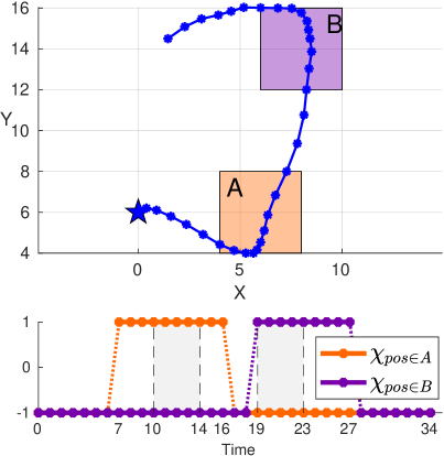
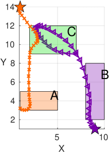
Scenario 1 - Timed Navigation. Consider an autonomous agent with 2D position and velocity where . We consider the dynamics
| (6) |
where and . The agent should first reach zone , see Fig. 2 for an illustration, any time within the time interval and then reach zone any time within as captured by the STL specification:
| (7) |
where and .
We first solve Problem 1 for and plot the resulting trajectory in Fig. 2(a), and obtain . From the characteristic function plotted in Fig. 2(a), one can see that if the agent starts the execution of the trajectory by up to 4 time steps earlier or later, the mission specification will still be satisfied, since for such a shifted trajectory there will be at least one point in time, where the agent is within zone and within the specified time intervals (depicted in grey color). This result supports Thm. III.2 derived previously. For comparison, the calculated left and right time robustness are and , respectively. One can see, that indeed, which is expected by Thm. III.4.
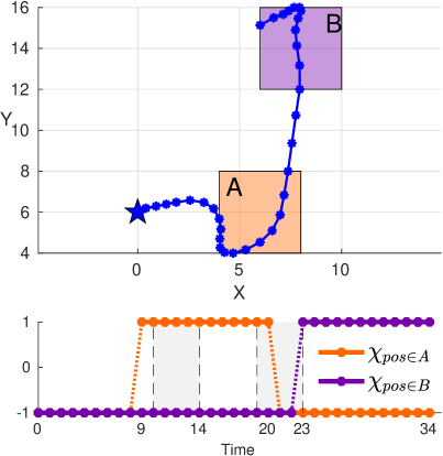
To compare the system’s behavior under different cost functions in Problem 1, we use the left time robustness and the right time robustness as control objectives. We next show that the temporal robustness is preferred over the left and right time robustness when dealing with systems where the direction of perturbations in time is unknown.
The results of maximizing the left time robustness are presented in Fig. 2(b) where . It is expected that the maximization of the left time robustness leads to a trajectory for which the agent reaches the desired goal within the required time bounds and then it stays there for as long as possible. In Fig. 2(b) this is represented as and . This means that if the agent starts the execution earlier by up to 10 time units (the trajectory is shifted to the left), the mission will still be satisfied. However, any perturbation that leads to a trajectory shifted to the right results in a violation of the specification, . Indeed, in this case, the agent will not be able to visit the zone within time units, see Fig. 2(b).
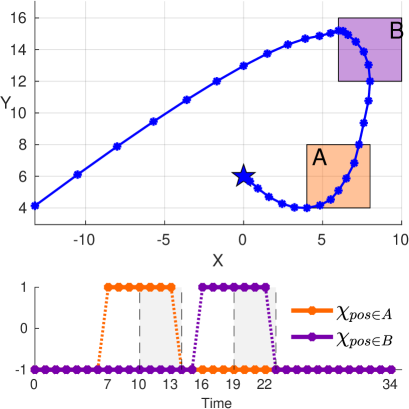
The results of maximizing the right time robustness are presented in Fig. 2(c) where . Note that in this case, the agent reaches both zones as soon as possible, see Fig. 2(c). We obtain the temporal robustness and left time robustness of . We can again see that which is consistent with Thm. III.4. Also note that since the evaluated left time robustness , only the predicate shifts up to time steps to the left still guarantee the satisfaction of the specification. From Fig. 2(c) one can see that the shift by time steps to the left leads to an agent leaving both regions of interest sooner than the predefined intervals, therefore, the mission is violated.
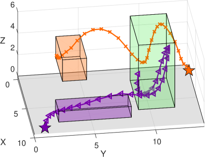
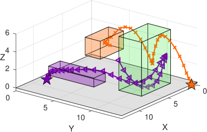
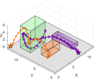
Scenario 2 - Timed Multi-UAV Surveillance. We now consider two unmanned aerial vehicles (UAVs) in a surveillance mission. Particularly, consider the th agent with state where pos and vel are the 3D position and velocity, see Fig. 3. The initial states are set to be and . Let the dynamics of both UAVs be of the form where and are obtained through the linearization of the UAV dynamics, see [31] for more details. The inputs are the thrust, roll, and pitch of the UAV.
The UAVs are tasked with a persistent surveillance mission of the region , see Fig. 3, while each of them must visit their individually assigned regions and . The overall specification is of the form where:
-
1.
UAV 1 should reach and stay in zone all the time from to time units, .
-
2.
UAV 2 should eventually reach zone any time between and time units, .
-
3.
Region should be surveilled, i.e. either one or both UAVs must be within all the time from to time units, .
Similarly to the 2D case, the regions , and are defined via a set of conjunctions over linear predicates.
We solve Problem 1 for the temporal robustness objective which leads to the optimal solution . Such optimal solution due to Thm. III.2 guarantees that for any shifted signal with , the mission specification will be satisfied. Take a look at Fig. 4. For the corner case, if one shifts the orange line to the left by time units and the violet one to the right by time units, i.e. , then one can see that and , therefore, . Analogously, and are satisfied by , therefore, the overall satisfaction of is indeed preserved by the shift .
VI Conclusions
We proposed a temporal robustness for STL specifications to account for forward and backward temporal perturbations. We showed the desirable properties of this new robustness notion, including soundness and the meaning of the temporal robustness in terms of permissible forward and backward time shifts. We then designed control laws for linear systems that maximize the temporal robustness objective using mixed-integer linear programming (MILP). Finally, we presented two case studies to illustrate how the proposed temporal robustness accounts for timing uncertainties.
References
- [1] O. Maler and D. Nickovic. Monitoring temporal properties of continuous signals. In Formal Techniques, Modelling and Analysis of Timed and Fault-Tolerant Systems, pages 152–166. Springer, 2004.
- [2] G. E. Fainekos and G. J. Pappas. Robustness of temporal logic specifications for continuous-time signals. Theoretical Computer Science, 410(42):4262–4291, 2009.
- [3] Y. Gilpin, V. Kurtz, and H. Lin. A smooth robustness measure of signal temporal logic for symbolic control. IEEE Control Systems Letters, 5(1):241–246, 2020.
- [4] P. Varnai and D. V. Dimarogonas. On robustness metrics for learning STL tasks. In 2020 American Control Conference (ACC), pages 5394–5399. IEEE, 2020.
- [5] V. Raman, A. Donzé, M. Maasoumy, R. M. Murray, A. Sangiovanni-Vincentelli, and S. A. Seshia. Model predictive control with signal temporal logic specifications. In 53rd IEEE Conference on Decision and Control, pages 81–87. IEEE, 2014.
- [6] A. T. Buyukkocak, D. Aksaray, and Y. Yazıcıoğlu. Planning of heterogeneous multi-agent systems under signal temporal logic specifications with integral predicates. IEEE Robotics and Automation Letters, 6(2):1375–1382, 2021.
- [7] V. Kurtz and H. Lin. Mixed-integer programming for signal temporal logic with fewer binary variables. IEEE Control Systems Letters, 6:2635–2640, 2022.
- [8] N. Mehdipour, C.-I. Vasile, and C. Belta. Average-based robustness for continuous-time signal temporal logic. In 2019 IEEE 58th Conference on Decision and Control (CDC), pages 5312–5317. IEEE, 2019.
- [9] Y. V. Pant, H. Abbas, R. A. Quaye, and R. Mangharam. Fly-by-logic: control of multi-drone fleets with temporal logic objectives. In 2018 ACM/IEEE 9th International Conference on Cyber-Physical Systems (ICCPS), pages 186–197. IEEE, 2018.
- [10] L. Lindemann and D. V. Dimarogonas. Control barrier functions for signal temporal logic tasks. IEEE control systems letters, 3(1):96–101, 2018.
- [11] M. Charitidou and D. V. Dimarogonas. Barrier function-based model predictive control under signal temporal logic specifications. In European Control Conference, Rotterdam, the Netherlands, accepted, 2021.
- [12] M. Cai, E. Aasi, C. Belta, and C.-I. Vasile. Overcoming exploration: Deep reinforcement learning in complex environments from temporal logic specifications. arXiv preprint arXiv:2201.12231, 2022.
- [13] A. Donzé and O. Maler. Robust satisfaction of temporal logic over real-valued signals. In Proceedings of the International Conference on Formal Modeling and Analysis of Timed Systems, 2010.
- [14] A. Rodionova, L. Lindemann, M. Morari, and G. J. Pappas. Time-robust control for STL specifications. In 2021 60th IEEE Conference on Decision and Control (CDC), pages 572–579, 2021.
- [15] A. Rodionova, L. Lindemann, M. Morari, and G. J. Pappas. Temporal robustness of temporal logic specifications: Analysis and control design. arXiv preprint arXiv:2203.15661, 2022.
- [16] T. Akazaki and I. Hasuo. Time robustness in MTL and expressivity in hybrid system falsification. In International Conference on Computer Aided Verification, pages 356–374. Springer, 2015.
- [17] J. V. Deshmukh, R. Majumdar, and V. S. Prabhu. Quantifying conformance using the skorokhod metric. In International Conference on Computer Aided Verification, pages 234–250. Springer, 2015.
- [18] H. Abbas, H. Mittelmann, and G. Fainekos. Formal property verification in a conformance testing framework. In 2014 Twelfth ACM/IEEE Conference on Formal Methods and Models for Codesign (MEMOCODE), pages 155–164. IEEE, 2014.
- [19] A. T. Buyukkocak and D. Aksaray. Temporal relaxation of signal temporal logic specifications for resilient control synthesis. arXiv preprint arXiv:2208.08384, 2022.
- [20] Y. E. Sahin, P. Nilsson, and N. Ozay. Synchronous and asynchronous multi-agent coordination with cLTL+ constraints. In 2017 IEEE 56th Annual Conference on Decision and Control (CDC), pages 335–342. IEEE, 2017.
- [21] Y. E. Sahin, P. Nilsson, and N. Ozay. Multirobot coordination with counting temporal logics. IEEE Transactions on Robotics, 36(4):1189–1206, 2019.
- [22] L. Lindemann, A. Rodionova, and G. Pappas. Temporal robustness of stochastic signals. In 25th ACM International Conference on Hybrid Systems: Computation and Control, pages 1–11, 2022.
- [23] D. Selvaratnam, M. Cantoni, J. Davoren, and I. Shames. MITL verification under timing uncertainty. arXiv preprint arXiv:2204.10493, 2022.
- [24] Z. Lin and J. S. Baras. Optimization-based motion planning and runtime monitoring for robotic agent with space and time tolerances. In 21st IFAC World Congress, pages 1900–1905, 2020.
- [25] C.-I. Vasile, D. Aksaray, and C. Belta. Time window temporal logic. Theoretical Computer Science, 691:27–54, 2017.
- [26] D. Kamale, E. Karyofylli, and C.-I. Vasile. Automata-based optimal planning with relaxed specifications. In 2021 IEEE/RSJ International Conference on Intelligent Robots and Systems (IROS), pages 6525–6530. IEEE, 2021.
- [27] F. Penedo, C.-I. Vasile, and C. Belta. Language-guided sampling-based planning using temporal relaxation. In Algorithmic Foundations of Robotics XII, pages 128–143. Springer, 2020.
- [28] H. Chen, S. Lin, S. A. Smolka, and N. Paoletti. An STL-based formulation of resilience in cyber-physical systems. arXiv preprint arXiv:2205.03961, 2022.
- [29] J. Lofberg. YALMIP: A toolbox for modeling and optimization in matlab. In 2004 IEEE international conference on robotics and automation (IEEE Cat. No. 04CH37508), pages 284–289. IEEE, 2004.
- [30] L. Gurobi Optimization. Gurobi optimizer reference manual, 2021.
- [31] T. Luukkonen. Modelling and control of quadcopter. Independent research project in applied mathematics, Espoo, 22:22, 2011.
APPENDIX
VI-A Proof of Theorem III.1
The proof is by induction on the structure of . We are going to prove the item 1. Item 2 can be proven analogously. We will also only show the predicate case, i.e., the case when . The other operators, i.e., when , can be done analogously to [14, Thm. 2.1].
Item 1. We must show . Since we are given that and in Def. III.1 , then and thus, since , .
VI-B Proof of Theorem III.2
Let be an STL formula built upon a predicate set , be a signal and be a time point. We want to show that for , such that , it holds that . The proof is by induction on the structure of .
Case . Denote . Then by Def. III.1, , . We get that , if , i.e., if . Since we assume that , then and thus .
Case . By definition, . We are given that . The induction hypothesis leads to . Thus, .
Case . We will only show the proof for the case when , since the case when can be shown analogously. Since , we know that for both and also due to Thm. III.1, and . Denote . Therefore, by Def. III.1, for both . We are given such that . Therefore since then by the induction hypothesis for both , for given it holds that . Thus, .
VI-C Proof of Theorem III.4
Let be an STL formula, be a signal, and be a time point. We want to prove that . The proof is by induction on the structure of .
Case . From Cor. III.3 we know that . Therefore, .
Case . Due to Def. III.1 and the induction hypothesis for , .