Combined tracer analysis for DESI 2024 BAO
Abstract
This paper demonstrates how the Dark Energy Spectroscopic Instrument (DESI) Data Release 1 (DR1) and future baryon acoustic oscillations (BAO) analyses can optimally combine overlapping tracers (galaxies of distinct types) in the same redshift range. We make a unified catalog of Luminous Red Galaxies (LRGs) and Emission Line Galaxies (ELGs) in the redshift range and investigate the impact on the BAO constraints. DESI DR1 contains of the final DESI LRG sample and less than of the final ELG sample, and the combination of LRGs and ELGs increases the number density and reduces the shot noise. We developed a pipeline to merge the overlapping tracers using galaxy bias as an approximately optimal weight and tested the pipeline on a suite of simulations, calibrated on the final version of the DESI Early Data Release. When applying our pipeline to the DESI DR1 catalog, we find an improvement in the BAO constraints of for and for consistent with our findings in mock catalogs. Our analysis was integrated into the DESI DR1 BAO analysis to produce the LRGELG result in the redshift bin, which provided the most precise BAO measurement from DESI DR1 with a 0.86% constraint on the BAO distance scale and a 9.1 detection of the isotropic BAO feature.
1 Introduction
Baryon Acoustic Oscillations (BAO) are sound waves that propagated in the photon-baryon plasma in the early Universe due to the competing effects of gravity and radiation pressure [1, 2, 3]. The opposing effects of these two forces created acoustic waves, which in turn moved the material into concentric shells with a characteristic radius based on the time these waves were able to travel until near the epoch of recombination. This radius represents a special scale in the distribution of matter (or galaxies), which can be used as a standard ruler to map out the expansion history of the Universe [4, 5]. Since the first detection of the BAO feature about 20 years ago [6, 7, 8], it has established itself as one of the most reliable low-redshift observables at redshifts in cosmology [9, 10].
BAO measurements have been reported in multiple galaxy redshift surveys from redshift [11, 12] to redshift [13] using galaxies and quasars, and at even higher redshift () using the Lyman-alpha forest [14]. Because the BAO is a very large-scale feature ( Mpc today), there are very few known processes that can easily remove or alter this signal. The large-scale bulk flow has been shown to dampen the BAO feature and shift its peak position [15, 16, 17, 18], with the effect being largest at low redshift. However, since the bulk flow (and the related displacement) is sourced by the density field, one can use the measured galaxy distribution to estimate the displacements and reverse most of these effects, a procedure known as density field reconstruction [19, 20]. Even though density-field reconstruction only works on linear and quasi-linear scales, it has been shown to improve the signal-to-noise ratio substantially, especially at low redshift, and effectively remove the shift in the BAO scale well below percent level [21, 22].
This paper is part of a series on the BAO analysis of the first data release (DR1) of the Dark Energy Spectroscopic Instrument (DESI). The DESI survey [23, 24] covers a very large redshift range from to using different tracers at different redshift intervals. This naturally leads to multiple tracers being present at the same redshift range. Here we investigate how best to combine such tracers in light of a BAO analysis. We focus on the redshift range where we have both Luminous Red Galaxies [LRGs, 25] and Emission Line Galaxies [ELGs, 26] available as tracers. An optimal analysis relies on combining the LRGs and ELGs for both the clustering estimator and the density field reconstruction. Studying the clustering signal of two different tracer types in the same volume also allows for tests of potential galaxy sample-specific systematic effects, including redshift space distortions, non-linear clustering and non-linear galaxy bias. Whereas most of these tracer-dependent effects have been studied carefully in N-body simulations (e.g. [27, 28, 29, 30]), systematic studies directly on the data have the advantage of relying on fewer assumptions, e.g., about the fiducial cosmology or the models for the galaxy-halo connection.
One interesting potential source of systematic bias for BAO is the relative velocity effect [31]. The fact that dark matter and baryons have a different velocity profile directly after decoupling can affect early galaxy formation processes. For example, wherever the relative velocity is large, baryons can escape the gravitational potential, reducing the chance of galaxy formation. Hence, the selection effects due to the relative velocity can introduce additional terms in the large-scale power spectrum [32]. Given that the relative velocity effect is sourced by pre-recombination physics, just like the BAO itself, this effect can bias BAO measurements if not accounted for. Investigations using the two-point and three-point clustering of the Baryon Oscillation Spectroscopic Survey (BOSS) and the WiggleZ Dark Energy Survey have not been able to detect this effect [33, 34, 35]. Testing such effects in mock datasets is challenging, as it requires understanding the impact of the relative velocity effect on galaxy formation processes. The tests on hydrodynamic simulations have detected the relative baryon-to-dark matter overdensity effect in galaxies [36], while tests on the Lyman alpha forest have shown that the effect there from the relative velocity effect is small but potentially important at DESI precision [37]. In [38], we include the estimated shift on the BAO scale for DESI galaxies and quasars in our systematic budget based on the former measurements, finding that the nonlinear shift due to the overdensity effect is dominant unless the relative velocity effect is at the very highest range explored in the literature. With the overlapping tracers, we can test the level of this systematics directly using the data.
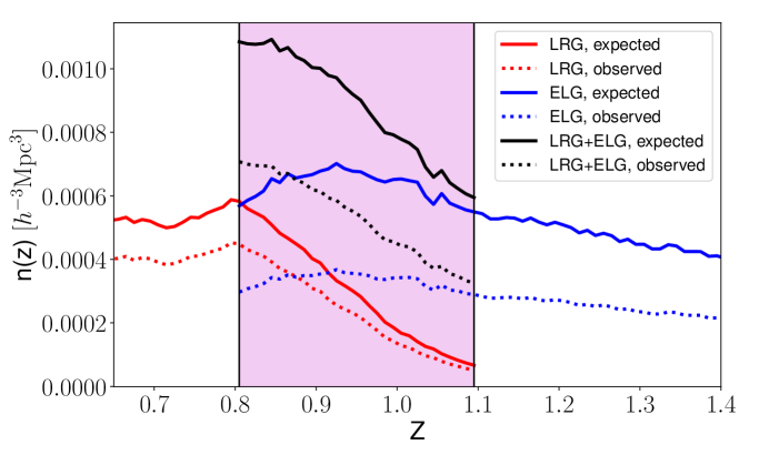
Combining the tracers into a unified catalog before the BAO analysis can have additional advantages compared to combining the BAO analysis results from multiple tracers. First, in case a tracer suffers from high noise, its BAO constraint would be weak with a highly non-Gaussian distribution. This is the case for the DR1 ELG sample at due to its low fiber assignment completeness (35.3%). The sample represents less than 1/4 of the final DESI ELG sample. Fig.˜1 shows the raw observed number density (dotted lines) and the expected number density corrected for completeness (solid lines); the difference between the two lines is much greater for ELGs than for LRGs, due to their low completeness. Besides, as we can see on the right panel of Fig.˜1, the clustering amplitude of ELGs is also lower. Both of these lower the signal-to-noise ratio of the BAO for ELGs, making the analysis suffer more from non-Gaussianity in the likelihood and less robust compared to other tracers. Second, the combined tracer clustering includes information from the auto-clustering statistics of the single tracers as well as the cross-clustering statistics between the tracers. The combination of tracers into a unified catalog before the clustering measurements and BAO analysis, therefore, enables a more robust (i.e., not impacted by non-Gaussianity of the single tracer ELG analysis) and complete (i.e., includes auto as well as the cross-clustering information with ELG) integration of the ELG information. Third, the lower shot noise of the combined tracer can potentially improve the reconstruction efficiency beyond the reconstruction of the individual tracers, especially for ELGs. This is why we expect the combination of the LRG and ELG catalogs over the overlapping redshifts to be beneficial to BAO analyses. Whereas we also have QSOs in this redshift bin, due to its very low sample density, the gain by including quasars in this combined tracer is expected to be marginal. Therefore, in this paper, we focus on the combined tracer of LRGs and ELGs. Based on the results presented in this paper, DESI DR1 BAO [39] adopted the combined tracer LRGELG as the baseline for this redshift bin.
The structure of the paper is as follows: in Section˜2 we briefly summarize the DESI DR1 dataset and the properties of the large-scale structure catalogs, focusing on the ELGs and LRGs . In Section˜3 we describe the DESI DR1 mocks we used for the tests in this paper. In Section˜4 we present how we construct the combined catalog, measure and analyze the clustering statistics, and perform the BAO analysis. In Section˜5 we assess the gain of the combined catalog using mocks as well as using DR1 data and test for systematics in the BAO measurements using the overlapping tracers. Finally, in Section˜6 we summarize the benefits of the combination of overlapping tracers and the prospects for future data releases.
2 DESI Data Release 1 (DR1)
The DESI instrument [40, 41] is located on the Mayall Telescope at Kitt Peak, Arizona. It can simultaneously observe up to 5000 targets using robotic positioners that precisely place optical fibers on the focal plane at the celestial coordinates of the targets [42, 43, 44, 45, 46]. The collected light is then carried out to one of the 10 spectrographs available. A set of targets at a specific sky position is collected through observations of ‘tiles’ [47]. DESI observing strategy is separated into two categories depending on the observing conditions. BGS observations are scheduled during “bright” time (with moonlight or during twilight), while QSO, LRG, and ELG targets are prioritized during “dark” time when the sky background is low. During these observations, the tracers compete for fiber assignment based on a predefined priority system designed to optimize science goals.
The galaxies observed in the DESI Data Release 1 (DR1, [48]) were collected during the main survey operations starting from May 14, 2021, after a period of survey validation [49], through to June 14, 2022. During this period, 2744 dark time tiles and 2275 bright time tiles were observed covering a surface area of order 7,500 deg2, just over half of the expected final coverage of 14,200 deg2. The observed data are processed by the DESI spectroscopic pipeline [50] daily for immediate quality checks. The redshift catalogs used for this analysis and released with DESI DR1 are obtained from a spectroscopic reduction run with a fixed pipeline version internally denoted as “iron”. From the redshifts and parent target catalogs, large-scale structure catalogs and two-point function measurements were made following the procedure described in [51, 52]. Along with the data, random sample catalogs (“randoms”), designed to account for the survey geometry, were also produced (cf. [47, 52, 51] for the detailed methodology). The redshift distributions are matched between data and randoms in each region separately (North or South Galactic cap — NGC/SGC).
One of the key science goals of DESI is to measure the BAO scale from redshift to redshift . To cover such a wide range of redshifts, DESI relies on different types of galaxies, which we will briefly introduce here. At the lowest redshift (), DESI observes a r-band magnitude-limited sample BGS, which has a significantly higher density compared to past surveys in this redshift range [53, 54, 55]. At higher redshift (), DESI observes LRGs, similar to the Baryon Oscillation Spectroscopic Survey (BOSS, [56]). At even higher redshift (), DESI observes ELGs, which make up the largest sample in DESI. ELGs suffer from low completeness (fiber assignment completeness is only 35.3% for DR1), due to the observing strategy of DESI, which favors quasars and LRGs during dark time. To go beyond redshift , DESI targets quasars. There are two different QSO selections: a homogeneous QSO selection up to redshift is designed for the study of the BAO feature in the QSO auto-correlation [39], and another QSO selection up to redshift is designed for the BAO study of the Lyman- forest [57].
| Tracer | (Gpc3) | |||
| LRG | 859,824 | 0.92 | 5.0 | |
| ELG | 1,016,340 | 0.95 | 2.0 | |
| LRG+ELG | 1,876,164 | 0.93 |
In this paper, we only focus on the LRGs, ELGs, and their combination (LRGELG) in the redshift range . Note that these correspond to LRG3, ELG1 and LRG3+ELG1 in [58] 111DESI DR1 analysis splits LRGs () into 3 redshift bins, LRG1, LRG2, and LRG3 and ELGs () into 2 redshift bins, ELG1 and ELG2. , respectively. Table˜1 provides some details on the properties of each sample, taken from [39]. Here represents the redshift at which the BAO fit parameters can be converted into physical distances and is calculated weighting by the square of the weighted number density of randoms (with the weights—including FKP222We follow the prescription from [59], which balances the cosmic-variance-dominated regions (high-density regions) and the shot noise-dominated regions (low-density regions) to minimize the variance.), :
| (2.1) |
where is the comoving distance to the redshift . The effective volume estimate is obtained for each redshift bin via
| (2.2) |
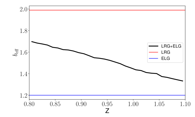
where are taken from Table˜1 and represent the amplitude of the observed power spectrum at the wave mode that is considered most relevant for the BAO information.333Values for are taken from [60]. Specifically, the ones that remove the effect of angular separations less than 0.05 degrees. was chosen to maximize the trade-off between area and number density at a fixed total number of objects for [61]. The comoving number density as a function of redshift for each sample is shown in the left panel of Fig.˜1. The right panel of Fig.˜1 shows the galaxy bias (right panel) of individual LRGs (red), ELGs (blue), and the weighted combination for LRGELG (black) in this redshift range (shaded region).
3 DR1 Mock catalogs
We utilize mock catalogs for multiple purposes. First, to test the realistic gain given the survey realism. Second, to identify any potential systematics when using the combined tracer. Third, to understand the expected range of consistency between the single-tracer and combined-tracer BAO measurements. The details of mocks are presented in various DESI DR1 papers [51, 39]; here, we summarize the key details once again to make this paper self-contained.
3.1 Abacus-2 DR1 mocks
The Abacus simulations are high-resolution gravity-only N-body simulations [62]. We use a set of 25 simulation boxes from the AbacusSummit suite [63], each with a volume of and particles. These AbacusSummit simulations assumed the Planck 2018 CDM cosmology, specifically the mean estimates of the Planck TT,TE,EE+lowE+lensing likelihood chains: , , , , , and [64]. This is also the fiducial cosmology used throughout the DESI DR1 analysis.
The Abacus-2 halos444Identified with the CompaSO halo finder [65]. are populated with galaxies using a flexible halo occupation distribution model (HOD) [66] which has been fitted to the galaxy two-point correlation functions of the final Early Data Release (EDR) [67, 68, 69] that included correction for all the systematics and included a detailed model for DESI focal plane effects. More details about the production and utilization of the mocks are provided in [39]. From these simulations, we create mock catalogs designed to mimic the survey realism, called “cutsky” Abacus-2 mocks, after applying the DESI footprint and survey selection function, including realistic redshift failures and targeting masks as described in [51]. As a caveat, the LRG DR1 mocks are produced using the simulation output at , while the ELG DR1 mocks were produced using the simulation output at [51]. In comparison, the actual effective redshifts of the two DR1 samples (LRG3, ELG1) are very close: 0.92 and 0.95, respectively (Table˜1). Despite the offset in the output redshifts of the mocks, the cross-correlations between the two tracers reasonably agree between the mocks and the data on the BAO scale, as will be shown in Section˜5 (Fig.˜4). We, therefore, ignore the effect of this redshift offset.
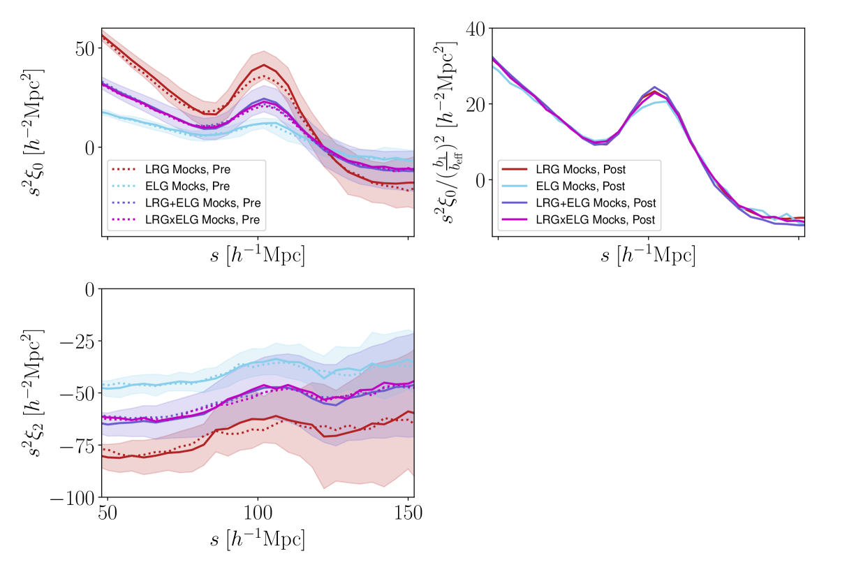
As the final step, fiber assignment in the mocks is modeled using the DESI fiber assignment pipeline, which replicates the actual survey tiling, priority, and collision logic. It is important to simulate this effect as it might bias our observation and so our BAO measurements. For details, see [52, 70]. This is called the ‘altmtl’ (the Alternate Merged Target Ledgers [71]) Abacus DR1 mocks. Even though they are more computationally expensive, they are the most realistic simulations of the DR1 data as they accurately reproduce DESI fiber assignments. Fig.˜2 shows the clustering amplitude of the DR1 mocks for LRG, ELG, their cross correlation LRGELG and their combination LRGELG.
3.2 EZmock DR1
The second type of mocks is based on the effective Zel’dovich approximation mocks [72], which we call EZmocks. EZmocks are almost as accurate as mocks on linear scales but less computationally expensive. We use 1000 realizations of DR1 EZmocks that are calibrated to produce two-point clustering statistics of Abacus-2 DR1, while constructed from a cubic volume of , as described in [39]. When applying the survey realisms to EZmocks, instead of applying and simulating fiberassign, we use the ‘fast-fiberassign (FFA)’ method that emulates the fiber assignment process by generating and averaging realizations from the average targeting probability as a function of number of overlapping tiles and local (angular) clustering, learned from the data. This ‘FFA’ method approximately reproduces the fiber-collisions pairwise incompleteness and is much faster than ‘altmtl’. We use these DR1 EZmocks only for the tests of the gain in BAO precision (Section˜5.1.2), which requires a greater number of independent simulations and needs to avoid a potential box replication effect 555To reach the full survey volume, the simulation box must be periodically replicated. This artificial tiling can introduce spurious large-scale correlations or suppress variance on scales approaching or exceeding the box size. [51]. The rest of the mock tests in this paper are performed using Abacus-2 DR1 mocks.
4 Methods
4.1 Nomenclature and fiducial cosmology
Our analysis requires an assumption of the fiducial cosmology for transforming the observational coordinates to the comoving coordinates and calculating the two-point correlation function, as well as in the BAO fitting. Whereas we use the Planck 2018 CDM cosmology as the DESI fiducial cosmology (Section˜3.1), the robustness against the choice of fiducial cosmology is extensively demonstrated in [73].
Throughout this paper, we follow the definition of from the DESI DR1 BAO analysis [39].:
| (4.1) | ||||
| (4.2) |
where is the sound horizon at the drag epoch, is the angular diameter distance, is the Hubble parameter, and and are the dilations along and across the line of sight, respectively. Quantities with the superscript “fid” are measured in the fiducial cosmology that we introduced above. Because also depends on , the two parameters are correlated at some level. It is useful in some cases to express the 2-D dilation in terms of the isotropic and anisotropic distortion parameters defined as
| (4.3) | ||||
| (4.4) |
where measures the spherically averaged BAO scale, and 666AP refers to the Alcock-Paczynski effect [74] i.e anisotropic distortion of the BAO feature. captures the anisotropy in the BAO feature.
4.2 Creation and weighting of the combined catalogs
The size and location of the BAO feature have been demonstrated to be approximately tracer-independent, especially after reconstruction [75, 76]. Therefore, the most naive approach to combining different BAO tracers is to concatenate the catalogs. However, given the different galaxy biases and sampling noise of the two tracers, an optimal approach would be to weight each tracer according to its signal-to-noise ratio when combining the catalogs. In this paper, we propose and test an approximate optimal weight assuming a scale-independent and isotropic signal-to-noise ratio. Once combined, we treat this as a single catalog, where the information it provides should be equivalent to or better than (especially if there is a gain during reconstruction) the combined information from all three clustering measurements available: the two auto-clustering measurements of the individual tracers and their cross-clustering. The cross-covariance among these three clustering statistics is naturally accounted for by treating them as a single catalog (at least within the approximation we use to derive the weight for the combination).
The ultimate information we want to derive from the combined tracer is the underlying matter density field (and the BAO feature in it) and the corresponding displacement field. LRG and ELG trace the underlying matter density field in a biased way. We construct an approximate maximum likelihood estimator of the matter density field, ignoring the anisotropies due to redshift-space distortions and scale-dependence of bias:
| (4.5) |
where and refer to the linear galaxy bias parameters for LRGs and ELGs, and are the observed number densities of LRG and ELG at a given location/pixel and and are the average number densities expected at given location/pixel, which are typically traced with randoms. The derivation for Eq.˜4.5 is presented in Appendix˜A.
Based on the estimator, we choose to weight each tracer with its estimated linear galaxy bias before merging the two catalogs. Then, the overdensity field of this combined catalog can be written as:
| (4.6) |
and the effective bias of this combined field is:
| (4.7) |
When comparing Eqs.˜4.6 and 4.7 with Eq.˜4.5, one can show
| (4.8) |
For simplicity, we ignore the position/redshift-dependence on when deriving the displacement field during reconstruction (Section˜4.4). But we account for the redshift-dependence of when updating the FKP weight for the combined tracer (Section˜4.2.2). The procedure for constructing the combined catalog can be summarized as follows:
-
1.
Estimate of the combined galaxy density field, assuming that each tracer is weighted with its estimated linear galaxy bias, and compute the new FKP weight based on it (Section˜4.2.2). This can be done without altering the clustering catalogs.
-
2.
In the clustering catalogs, weight LRGs with and ELGs with , i.e., multiply the existing clustering weight by the corresponding bias for each galaxy. Weight the random particles in the same way.
-
3.
Renormalize the randoms so that the data-to-randoms weighted sum ratio is the same for both tracers. See Section˜4.2.3.
-
4.
Concatenate the two galaxy catalogs with the new weights (with biases, the new FKP weight). Do the same to the randoms (with the additional renormalization).
In the following subsections, we present practical details of each step for interested readers.
4.2.1 Single-tracer weights for galaxies and randoms
As we mentioned in Section˜2, each data and random in the DESI catalogs is associated with a set of weights; ("WEIGHT" column in the catalog file) corrects for the variations in the selection function and the FKP weight, ("WEIGHT_FKP" column), is designed to construct a minimum variance power spectrum estimator given the redshift-dependent number density. Each source is then multiplied by the net weight :
| (4.9) |
The FKP weight is defined as
| (4.10) |
where 777For details of , please refer to [51]. is the mean tile completeness at a given (discrete) number of overlapping tiles , is the expected comoving number density (solid lines in Fig.˜1), , is the actual, observed comoving number density (dashed lines in Fig.˜1), and represents an approximate value of the power spectrum monopole at . It is used as a reference amplitude in the FKP weighting scheme, and is set to for Luminous Red Galaxies (LRGs) and for Emission Line Galaxies (ELGs) in DESI DR1 [51].
Since we want to treat the combined catalog as a single tracer after weighing each tracer with its linear bias, we need to redefine effective FKP weights for the combined sample.
4.2.2 Updating the FKP weights
Here we are going to describe how we derive the combined quantities leading to the effective FKP weights:
-
1.
First we split the complete redshift range of the two tracers (with an overlap between . See Fig.˜1) in bins of . We then construct the effective redshift-dependent bias from
(4.11) where , stand for the expected comoving number density, and , for the linear bias assumed for LRG and ELG, respectively. The extra factor of and in the numerator reflects each tracer being weighed with its own .
-
2.
Now that we have the effective bias, the next step is to derive the effective comoving density distribution as follows:
(4.12) -
3.
Based on the mean when averaged over all sources between , we choose for LRGELG. Given the formula of the FKP weights, we derive the new effective FKP weight:
(4.13) is position-dependent in a way that is specific to the type of the tracers so that would be calculated differently between LRG targets versus ELG targets within the concatenated catalog, despite the common : and . Therefore, although combined, we are weighing different tracers in the same location slightly differently depending on their tiling completeness888Ideally, we would use in the denominator of Eq. 4.13, where for each tracer..
4.2.3 Re-weighting and concatenating the catalogs
Before combining, we first update the weight () by multiplying it with the estimated linear bias for each tracer . Then, with the new FKP weight (Eq.˜4.13), the weight assigned for data and randoms inside this combined catalog is:
| (4.14a) | ||||
| (4.14b) | ||||
| (4.14c) | ||||
Here , and corresponds to the WEIGHT in the original catalogs. Note that we renormalize the weights for ELG randoms to match the LRG (weighted) data-to-random ratio999Symmetric weight renormalization for both randoms must give equivalent results. Still, we prioritize exact documentation of the DESI DR1 combined catalog production.. This relative normalization ensures that when the combined random catalog is normalized to match the weighted sum of the combined tracer catalog, the weighted sum of randoms for each tracer also matches that of the corresponding tracer. Without this step, the combined randoms might misrepresent the combined catalog’s selection function due to the tracers’ different structures. We then merge all these sources into a single catalog.
4.3 Two-point correlation function
Following the pipeline defined in [39, 77], the correlation functions are computed using the Landy-Szalay estimator [78]
| (4.15) |
with being the cosine of the angle between the galaxy pair and the line of sight, refer respectively to points from the data and random catalogs, and is the pair separation (here we use bins with a width of ). To compute the two-point correlation we use the publicly available code pycorr101010https://github.com/cosmodesi/pycorr [79] based on the Corrfunc111111https://github.com/manodeep/Corrfunc engine [80, 81]. For our analyses, we convert the output to Legendre multipoles (specifically the monopole () and the quadrupole ()). To extract the maximum out of the clustering measurement, we weigh each galaxy by a combination of weights, as described in Section˜4.2 (Eq.˜4.14 for the combined tracer, analogous to Eq.˜4.9 for regular single tracers).
Since the data reduction produces catalogs for each of the galactic caps, we choose to compute the correlation functions for NGC and SGC separately. Accordingly, we perform the catalog combination separately for NGC and SGC. Then the combination is performed by summing the pair counts computed in each region independently. This allows us to compare the consistency of the two regions and test for possible systematics. In some cases, an insufficient number of randoms can degrade the computation of the two-point statistics. To avoid this, we concatenate multiple random catalogs (typically 18) so that the number of randoms is more than 50 times the number of data galaxies.
4.4 Density field reconstruction and specific configuration
We apply the density field reconstruction technique [82] on the catalogs considered in this paper, single and combined tracers, to partially recover the BAO feature that has been degraded due to structure growth and redshift-space distortions (RSD). We follow the DESI DR1 default reconstruction setup in [39], which was determined based on a set of extensive tests in [77, 83].
To summarize, we use pyrecon,121212https://github.com/cosmodesi/pyrecon a Python package developed by the DESI collaboration, and adopt IterativeFFTReconstruction (hereafter, ‘IFFT’) that implements the iterative procedure described in [84], with the RecSym convention. 131313RecSym is a choice to recover the large-scale anisotropy due to redshift-space distortions in the process of reconstruction. The overdensity field is smoothed by a Gaussian kernel of width for all of the tracers we consider in this paper. For reconstruction, we use the linear bias in Table˜2 and the growth rate in Table˜1. The value of linear bias, , is computed from Eq.˜4.11 where the formula is integrated over the redshift range.
| Tracer | Linear bias | Growth rate | Reconstruction range | ||||
| Pre-recon | Post-recon | Pre-recon | Post-recon | ||||
| LRG | 4.5 | 3.0 | 9.0 | 6.0 | 2.0 | 0.83 | 0.4 – 1.1 |
| ELG | 4.5 | 3.0 | 8.5 | 6.0 | 1.2 | 0.90 | 0.8 – 1.6 |
| LRG+ELG | 4.5 | 3.0 | 9.0 | 6.0 | 1.6 | 0.87 | 0.8 – 1.1 |
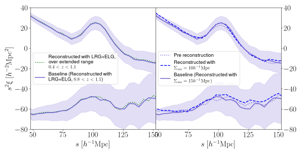
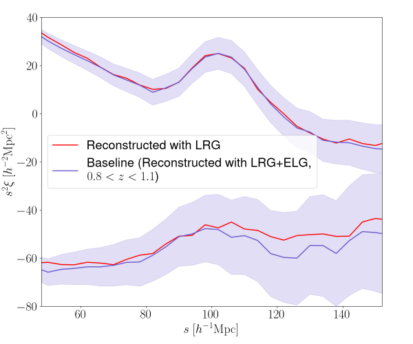
As a caveat, whereas the default reconstruction setup of the individual tracers is performed using the displacement field constructed over the full redshift range for LRG and ELG, i.e., for LRG and for ELG, the reconstruction of the combined catalog is performed using the displacement field estimated from , i.e., the range where the two tracers overlap, as stated in [39]. The latter choice was made to input bias and growth rate that are better representative of the overlapping sample to the reconstruction pipeline, rather than using an effective bias and the growth rate averaged over a wide range of redshift (i.e. or ). The downside of this choice is a potentially greater boundary effect at when estimating the displacement field across the boundaries. The left panel of Fig.˜3 shows the mean correlation functions of five LRGELG mocks over using the displacement field constructed from (green-dotted, the convention used for LRGs) and from (blue, our default choice for LRG+ELG). The figure shows that the choice of the reconstruction redshift range between the two options has little impact on the reconstructed correlation function. Therefore, the comparisons of LRG and the combined tracer in this paper are minimally impacted by the different reconstruction redshift ranges.
In the right panel, we also test the effect of the Gaussian smoothing kernel for reconstruction. Given the effective number density of the combined tracer, greater than LRG and ELG, we test a more aggressive kernel (dashed blue line): the gain of using a smaller smoothing kernel does not appear obvious in the BAO feature of the monopoles, which mainly determines the constraint on . While there is a slight difference in the quadrupole, based on the little visible impact on the monopole, we adopt that is the default for DR1 LRG and ELG samples.
For the cross-correlation LRGELG of LRG and ELG, we cross-correlate after each of LRG and ELG is separately reconstructed. One could also use the cross-correlation of the two tracers after reconstructing using the common, combined displacement field, especially given the potentially noisy displacement field from ELG alone. For a more conservative systematic/consistency check, we, however, decided to cross-correlate the individually reconstructed two fields, which can be subject to more errors.
4.5 Covariance matrices
| Name | Tracer | Notes |
| RascalC-LRG | LRG | RascalC calibrated on DR1 LRG clustering (pre and post) |
| RascalC-ELG | ELG | RascalC calibrated on DR1 ELG clustering (pre and post) |
| RascalC- | LRGELG | RascalC calibrated on DR1 LRG, LRGELG and ELG clustering (only post-recon) |
| RascalC-comb | LRGELG | RascalC calibrated on DR1 LRGELG clustering (pre and post) |
In this work, we used semi-analytical covariance matrices for the 2-point correlation function multipoles produced with the RascalC code141414https://github.com/oliverphilcox/RascalC [85, 86, 87, 88, 89]. It computes the covariance matrix terms based on an empirical 2-point function (but not 3- and connected 4-point functions) and applies a shot-noise rescaling to mimic non-Gaussian effects. We refer the readers to [89] for further details on the methodology.
The covariance matrix for the combined tracer was produced similarly to other single tracers, using the combined data and random catalogs151515Scripts are available at https://github.com/misharash/RascalC-scripts/tree/DESI2024/DESI/Y1/comb.. Therefore, the LRG, ELG and LRGELG RascalC covariance matrices in this paper are the same as in the main DESI 2024 galaxy BAO analysis [39]. The covariance matrix of the cross-correlation function (LRGELG) was produced based on data correlation functions and random catalogs according to Appendix A of [89]161616Scripts are available at https://github.com/misharash/RascalC-scripts/tree/DESI2024/DESI/Y1/cross., using the shot-noise rescaling values calibrated with jackknives on LRG and ELG auto-correlations. Table˜3 summarizes the covariances we use in this paper.
4.6 BAO fitting
The BAO fitting procedure for the DESI collaboration is based on the extensive tests that are summarized in [38]. The model consists of a combination of a physically motivated model from quasi-linear theory and a parameterized model to marginalize over non-linearities that may otherwise affect our measurements of the BAO scale. For interested readers, [39, 38] explain the fitting model for different choices of the reconstruction convention, how the power spectrum multipoles are transformed into configuration space multipoles, the broadband modeling and its marginalization, etc. Here we simply show in Table˜4, a few of the parameters of interest.
To summarize, we use a mixture of flat () and Gaussian priors (damping terms). To isolate the BAO feature, the range of galaxy separation is restricted to . The fit is performed with the publicly available code on two-point correlation functions of combined galactic caps (NGC+SGC) using the desilike171717https://github.com/cosmodesi/desilike. Fitting methods available are MCMC sampling (e.g. emcee [90], pocoMC [91]) or posterior profiling (MINUIT [92]). The software offers the possibility to fit in several parameter spaces. In this paper, we chose to present our results in or .
| Parameter | prior | Description |
| [0.8, 1.2] | Isotropic BAO dilation | |
| [0.8, 1.2] | Anisotropic (AP) BAO dilation | |
| Transverse BAO damping [] | ||
| Line-of-sight BAO damping [] | ||
| Finger of God damping [] | ||
| Fitting range | [48, 152] | Measurement bin edges |
| Data binning | Measurement bin width |
For the priors on the damping parameters, the central values denoted by the superscript ‘fid’ are tracer-specific and they are shown in Table˜2. These fiducial values are motivated by a combination of theoretical calculations, measurements of the cross-correlation between the initial and post-reconstruction density fields, and fits to mock catalogs. Finally, the total number of free parameters for our 1D and 2D fits is 7 and 13, respectively, for . The corresponding numbers of degrees of freedom for our 1D and 2D fits are 19 and 39.
5 Results
In this section, we demonstrate that our method of combining tracers yields an unbiased BAO estimator and mildly enhances the precision compared to the single catalog. After validating the method with the mocks, we apply it to the DR1 data, quantify the gain, and test for potential tracer-dependent systematics in the BAO measurements by comparing different tracers, including the cross-correlation LRGELG.
5.1 Application to the DESI DR1 mock catalogs
We first apply our pipeline on the 25 Abacus-2 DR1 mocks and estimate the expected level of systematics and the gain from the combination of catalogs.
In Fig.˜4 we show the mean of the correlation function for the 25 realizations of pre- and post-reconstruction for LRGs, ELGs, LRGELG, and LRGELG. The amplitude of clustering is proportional to the product of the galaxy biases of the two samples, and we can estimate the galaxy bias of LRGELG and LRGELG from LRG () and ELG () 181818The default bias values for LRG and ELG are taken from [39].. One can see a clear BAO feature around the 100 with a slightly sharper peak after reconstruction (a sign that some of the non-linearities have been successfully corrected). This is especially the case for LRG and LRGELG. The ELG reconstruction was likely hindered by its low completeness, which should be improved with future data releases of the DESI survey.
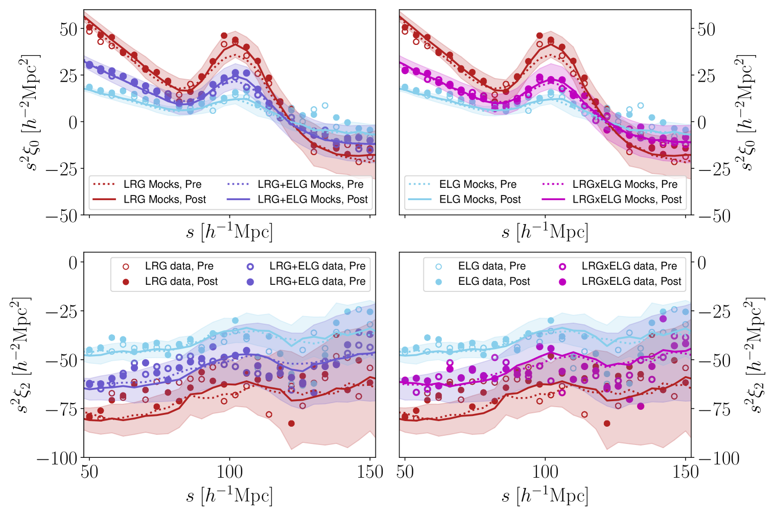
5.1.1 Effects of tracer combination on the reconstruction efficiency
One of the advantages we are seeking by using the combined tracer is to leverage the lower shot noise of the combined tracer to potentially improve the reconstruction efficiency beyond the reconstruction of the individual tracers. On the other hand, DESI DR1 ELG over suffers a much larger residual observational systematics [51, 93] in addition to the higher shot noise associated with its low completeness, which could end up increasing undesired systematics when combined to estimate the displacement field.
Therefore, we first investigate the impact of ELGs in the displacement field calculation. In Fig.˜5, we test the reconstruction of the combined catalog using the displacement calculated with LRG density fields (red line, i.e., without ELG), in comparison to the default case using the displacement fields from the combined catalog (black line). We find little difference in the BAO feature in the monopole, implying that most of the signal in the displacement field is coming from LRGs and that ELGs do not significantly impact reconstruction. That is, the primary benefit of the combined tracer for DR1, relative to LRGs alone, appears mainly to be the stable and robust integration of the low signal-to-noise ELGs by constructing a unified catalog before the BAO analysis, without an obvious additional gain in the reconstruction efficiency. We will revisit this quantitatively by comparing the reconstruction efficiency of LRGELG in terms of the BAO constraint in the following section.
5.1.2 The impact on the BAO constraints
We perform a two-dimensional fit using the monopole and quadrupole of the simulations and constrain BAO scales in the basis of the isotropic and anisotropic , and equivalently, in the basis of the radial () and perpendicular () directions. We estimate the precision in terms of the dispersion of the 191919Here refers to the number of realizations of Abacus-2 DR1 mocks best fits and the average of the likelihood errors , as presented in Table˜5. We also present the correlation coefficient between the isotropic and anisotropic parameters , and the chi-square per degrees of freedom .
| Tracer | Recon | ||||||||
| LRG | Pre | 0.9989 | 0.0143 | 0.0133 | 1.0037 | 0.0322 | 0.0491 | 0.1278 | 52.0/39 |
| ELG | Pre | 1.0014 | 0.0322 | 0.0282 | 0.9840 | 0.0495 | 0.0755 | -0.2354 | 41.4/39 |
| LRGELG | Pre | 1.0000 | 0.0159 | 0.0133 | 0.9916 | 0.0433 | 0.0463 | 0.0043 | 44.7/39 |
| LRG+ELG | Pre | 0.9998 | 0.0148 | 0.0120 | 0.9937 | 0.0374 | 0.0433 | 0.0803 | 39.4/39 |
| LRG | Post | 0.9956 | 0.0094 | 0.0097 | 0.9926 | 0.0240 | 0.0339 | 0.0388 | 42.1/39 |
| ELG | Post | 0.9977 | 0.0235 | 0.0250 | 1.0000 | 0.0492 | 0.0680 | -0.4545 | 40.9/39 |
| LRGELG | Post | 0.9973 | 0.0136 | 0.0108 | 0.9979 | 0.0318 | 0.0359 | -0.1340 | 43.0/39 |
| LRG+ELG | Post | 0.9971 | 0.0108 | 0.0086 | 0.9983 | 0.0258 | 0.0294 | -0.0188 | 39.9/39 |
| LRGEZ | Post | 0.9993 | 0.0100 | 0.0101 | 0.9996 | 0.0329 | 0.0343 | 36.8/39 | |
| LRG+ELGEZ | Post | 1.0001 | 0.0083 | 0.0088 | 1.0005 | 0.0270 | 0.0294 | 32.1/39 |
First, we inspect the efficiency of reconstruction between the single and the combined tracers. Table˜5 shows that, as expected from Fig.˜4, reconstruction improves the precision of our BAO measurements. Both the dispersion and the mean likelihood error show improvement for and : by 40% for LRGELG for both BAO parameters, a level of improvement similar to LRG. Since the improvement fraction in reconstruction is not larger for LRGELG than for LRG alone, we again do not find an obvious gain from constructing the combined displacement field during reconstruction. The cross statistics after reconstruction, LRGELG present a reconstruction improvement of .
We next estimate the net gain of constructing a combined catalog relative to the LRG catalog alone. The effective volumes ( for LRGELG and for LRG according to Table˜1) predicts about 14% improvement between LRGELG and LRG (assuming no additional gain during reconstruction). Given that cosmology constraints from ELG at this redshift bin were excluded from the DESI DR1 analysis [39, 94] due to their low signal-to-noise, this modest improvement makes a case for using the combined tracer.
We want to confirm this gain by inspecting the BAO constraints, and/or of simulations. If the likelihood distribution of the parameter is perfectly Gaussian, two estimates of precision should match in the infinite sample limit. With the 25 realizations, unfortunately, the typical dispersion associated with the standard deviation of 25 samples, , is expected to be as large as 14% 202020 with ., which is the level of gain we want to prove. Also, Abacus-2 DR1 mocks potentially suffer the box replication effect due to it being constructed from a box size of . On the other hand, reflects the property of the DR1 data through the DR1 covariance matrix, which may not perfectly resemble the dispersion of the mocks in a way that depends on tracers. For example, and of Abacus-2 LRG shows a difference of a factor of 1.4. We therefore cannot be confident that the from Abacus-2 DR1 should be sufficiently precise or consistent with . Table˜5 indeed gives inconclusive implications about the gain, being different depending on and 212121The gains were calculated by dividing the difference in precision by the precision of the LRG case..
To increase the statistical precision of this comparison without the box replication effect, we adopt 1000 DR1 EZmocks that were constructed from simulation boxes. The estimation of gains based on (last two rows of Table 5) now allows the statistical comparison at the level of 2% 222222As LRGELG and LRG are covariant, this 2% does not directly translate to the precision of comparing the two constraint values.. With , we find a gain in both BAO parameters with LRGELG over LRG, 17% for and 11% for . This is primarily because LRG from 1000 EZmocks is much more consistent with its , likely due to reduced sample variance, unlike the large discrepancy seen with 25 Abacus-2, which results in coherent gain with LRGELG over LRG for both and .
We next focus on that reflects the gain expected given the variance of the DR1 data. Note that the variance of DR1 is shown to be different from the variance of the EZmock; higher by 1.22-1.25 (i.e., 11-12% larger values in error) [51, 95] mainly due to the approximation in the fiber assignment process in EZmock. For LRGELG of 1000 EZmock, is greater than for both and by , i.e., being fairly consistent after accounting for the expected variance difference between EZmock and the DR1 data [51, 95].
With 1000 EZmocks, the overall gain of LRGELG over LRG in is 13% for both and , well-aligned with the difference and with the 17% (11%) gain in terms of (). This is also consistent with the gain estimated using Abacus-2 : 11% (13%) for (). We therefore consider Abacus-2 DR1 as a more reliable measure of precision than for the rest of the paper. Fig.˜6 shows the gain distribution from the 25 DR1 mocks.
5.1.3 Testing BAO systematic errors using the overlapping tracers
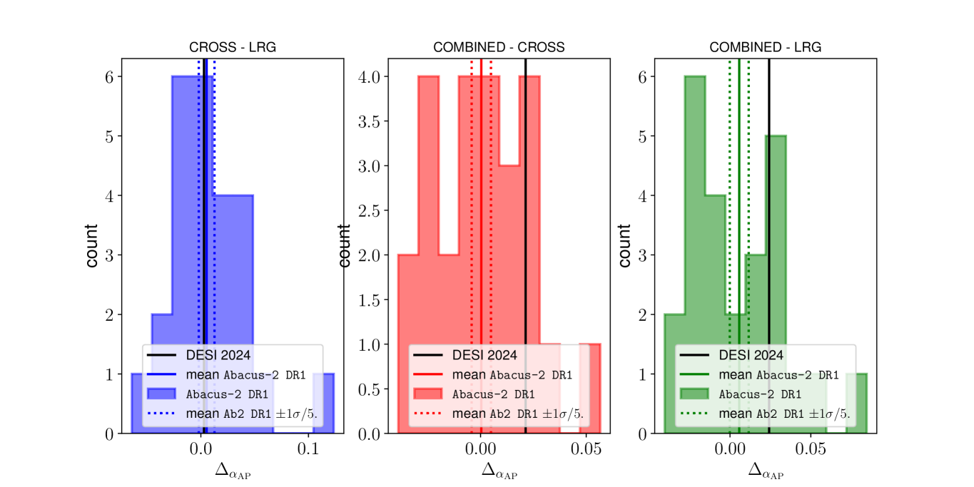
The best fit post-reconstruction BAO values of Abacus-2 in Table˜5 demonstrate that LRGELG as well as LRGELG return unbiased estimates of the BAO scales, all within , where is the significance defined in terms of the typical dispersion of the average differences of the mocks 232323 where is the number of realizations.. This validates the use of LRGELG as well as LRGELG as the BAO tracers. Note that the offset from the unity in LRG was discussed in [39], and considered non-detection of systematics, as it does not pass the threshold.
With multiple unbiased BAO tracers for this redshift bin, we can test the consistency among the BAO measurements. A disagreement between the BAO scales in real data can potentially indicate a tracer-dependent source of systematics, either due to observational artifacts or due to a cosmological effect such as the relative velocity effect [31]. Since the tracers are correlated, tracing the same underlying matter distribution with a different clustering bias, this consistency test can benefit from the sample variance cancellation. Using Abacus-2, we first test how much consistency is expected between the different but correlated tracers due to statistical fluctuations, in the absence of unknown systematics. As a reminder, these mocks include the fiber assignment effects ‘altmtl’, the level of which is different between ELG and LRG, but do not include any other observational systematics. The impact of the observational systematics, such as the imaging systematics and spectroscopic systematics, was shown to be negligible in [39].
| Estimates | Recon | ||||
| Post | 0.209 | 0.458 | 0.743 | 1.178 | |
| Post | 0.169 | 0.228 | 0.533 | 0.730 | |
| Post | 0.156 | 0.159 | 0.568 | 0.586 | |
| Post | 0.0017 | 0.0028 | 0.0036 | 0.0276 | |
| Pre | 0.252 | 0.554 | -1.973 | 0.985 | |
| Pre | 0.106 | 0.280 | -1.207 | 0.599 | |
| Pre | 0.083 | 0.197 | -1.005 | 0.518 | |
| Pre | 0.0014 | 0.0053 | 0.0385 | 0.0334 |
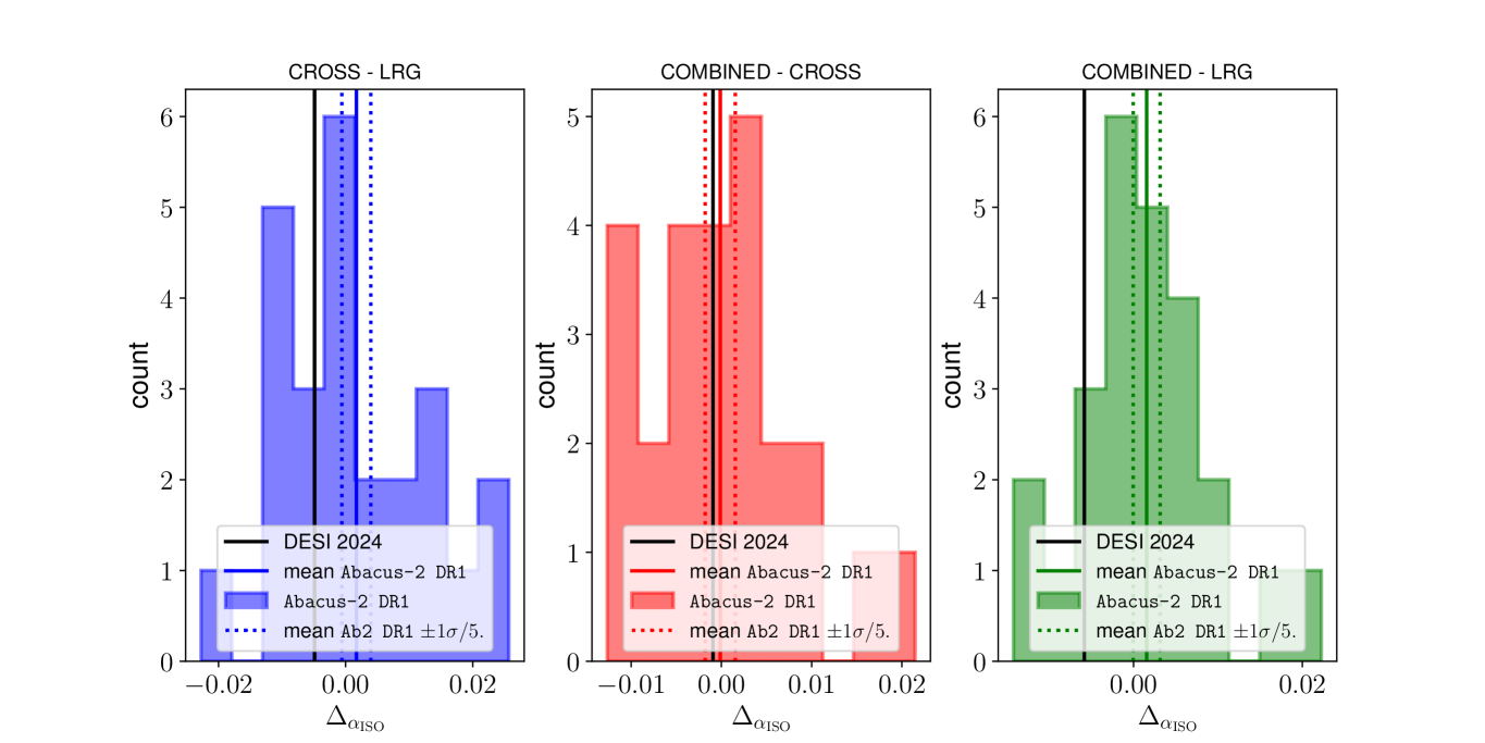
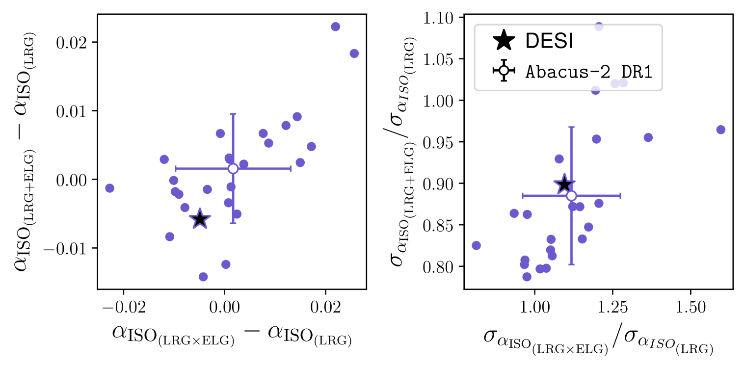
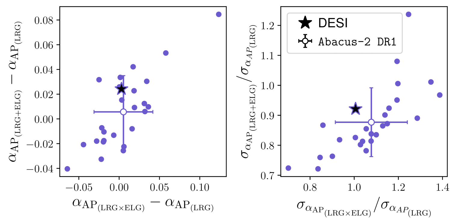
Table˜6 presents the average and the dispersion of the differences between different BAO tracers. The dispersions are divided by with to represent the error associated with the average difference. In Fig.˜7 we compare (left panel in blue), (middle panel in red) and (right panel in green) for and . For every case, the differences are expected to be zero within the statistical precision; the mean of the mocks (solid colored vertical lines) agrees with zero difference within of the statistical precision associated with the mean (vertical dashed lines). The next section compares the differences measured from the DESI DR1 data with the expectation.
5.2 Application to the DESI DR1 data catalog
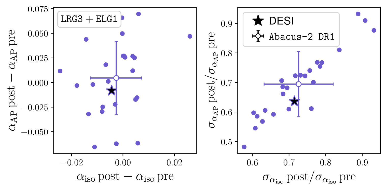
The last step of our analysis is to apply the combined tracer analysis on the DR1 data and investigate the gain and potential systematics. In Table˜7, we present the results of BAO fits applied to the DESI DR1 data. First, Fig.˜8 repeats one of the sanity checks presented in [39]: pre- and post-reconstruction BAO measurements for LRGELG, comparing DESI DR1 measurements (stars) with the 25 Abacus-2 DR1. Therefore, the reconstruction efficiency of DESI DR1 LRGELG is consistent with what is expected from the mocks.
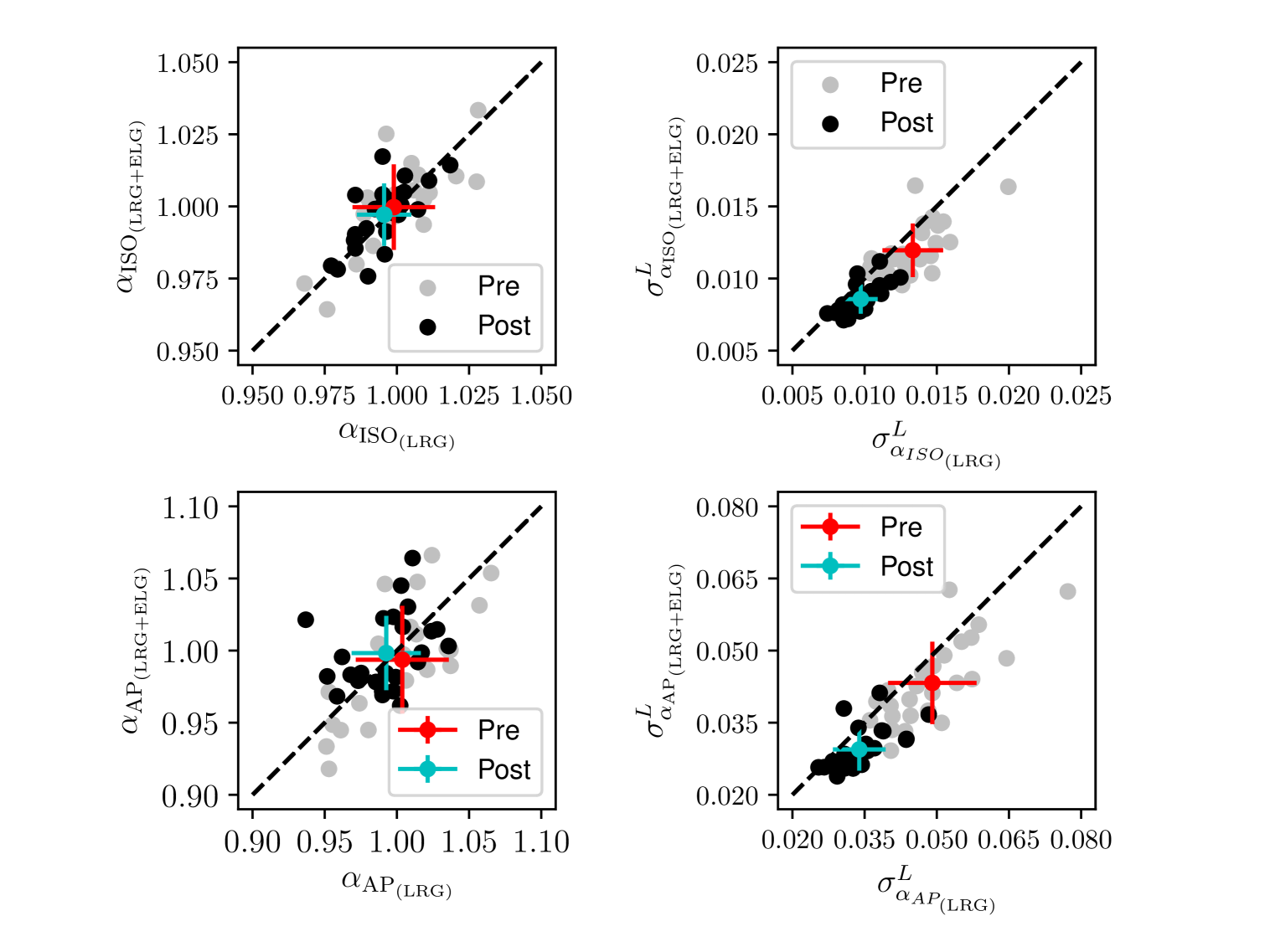
In terms of a gain in precision between LRGELG and LRGs, Table˜7 shows that, for we find a gain of pre recon and post reconstruction, while the gain for is pre recon and post reconstruction. Fig.˜9 visualizes that post-reconstruction BAO measurements between LRG and LRGELG (y-axis) as well as LRG and LRGELG (x-axis) fall within the distribution of the mocks. Especially, the gain in precision of the combined tracer observed from the data (right panels) is consistent with the gain in terms of of the Abacus-2 mocks.
Fig.˜7 shows differences in ’s from pairs of the BAO tracers, including LRGELG, comparing those of the mocks to the data. All differences from DR1 data are within the range of the histograms, therefore consistent with zero offsets, and therefore no indication of a tracer-dependent systematics/physics242424Since we are testing a single realization, DR1, we compare the DR1 constraint with the entire width of the distribution, instead of the width divided by .. As a caveat, while LRGELG returns consistent precisions compared to the mocks, the data returns much higher than the average of the mocks in Table˜5. Although this implies may need a more careful inspection in terms of the goodness of the fits, we defer such a test to future study.
| Tracer | Redshift | Recon | ||||
| LRG | 0.8–1.1 | Post | 0.0090 | 0.0299 | -0.0597 | 46.2/39 |
| LRGELG | 0.8–1.1 | Post | 0.0081 | 0.0278 | -0.1019 | 33.1/39 |
| LRGELG | 0.8-1.1 | Post | 0.0099 | 0.0303 | -0.4203 | 63.5/39 |
| ELG | 0.8–1.1 | Post | 0.0200 | 20.4/19 | ||
| LRG | 0.8–1.1 | Pre | 0.0120 | 0.0446 | 0.2737 | 48.4/39 |
| LRGELG | 0.8–1.1 | Pre | 0.0114 | 0.0436 | 0.2569 | 53.0/39 |
| LRGELG | 0.8-1.1 | Pre | 0.0126 | 0.0473 | 0.2987 | 48.3/39 |
| ELG | 0.8–1.1 | Pre | 0.0620 | 29.2/19 |
6 Conclusion
In this paper, we presented how the Dark Energy Spectroscopic Instrument (DESI) current and future BAO analyses can optimally combine overlapping tracers in the same redshift range. We focused on the two tracers, DESI DR1 Luminous red galaxies (LRGs) and Emission line galaxies (ELGs) in the redshift range and investigated the impact of the combined tracer on the BAO constraints.
The combination of tracers into a unified catalog enables a more robust integration of the two tracers, including the information from the cross-correlation of the two tracers. This paper presented a simple method of combining the two catalogs and tested the robustness of the combined catalog as a BAO tracer. In parallel, we tested if the lower shot noise of the combined tracer could potentially improve the reconstruction efficiency beyond the reconstruction of the individual tracers. We also tested if the different tracer types in the same volume allow for tests of potential tracer-dependent systematic effects, either observational or physics missing in our model, such as the relative velocity effect.
We find that due to the low completeness of DR1 ELGs, the combined LRGELG tracer does not exhibit a clear gain in reconstruction efficiency compared to that of the dominant tracer, LRG. Instead, it achieves a similar level of efficiency. We expect future DESI data with higher ELG completeness near the final DESI dataset to yield improved displacement field estimates.
We observe a gain of of improvement in the BAO precision with the combined tracer, which appears to be consistent with the additional information from the ELG BAO feature. Therefore, the main advantage of the combined tracer over LRGs alone in DR1 is its stable and complete integration of low–S/N ELG data through a unified pre-analysis catalog, naturally incorporating auto- and cross-clustering to maximize information extraction. This benefit remains applicable to future data releases with a higher S/N ELG as well and is indeed utilized in [96, 97, 98].
Using DR1 mocks, we demonstrate that the combined tracer LRGELG constructed using our method, as well as the cross-statistics, LRGELG, are unbiased tracers of BAO post-reconstruction in the presence of the simulated survey realism. Using these BAO tracers from the DR1 data in addition to LRG and ELGs, we tested for the systematics on the BAO scale at the redshift range of and found results that are consistent with no tracer-dependency between different tracers. That is, we detect neither the net effect of systematics nor the effect of relative velocity effects, within the statistical precision of DR1. With DR2, we revisit and extend the set of tests to other tracers and redshift ranges [98].
The method presented in this paper was integrated into the DESI DR1 BAO analysis to produce the LRGELG at the redshift bin of , which provided the most precise DESI BAO measurement of DR1 with a 0.86% constraint on corresponding to a 9.1 detection of the isotropic BAO feature.
Data Availability
Data Release 1 is available at https://data.desi.lbl.gov/doc/releases/. Additional clustering data and Python scripts used to produce the figures presented in this manuscript will be made available.
Acknowledgments
DV and H-JS acknowledge support from the U.S. Department of Energy, Office of Science, Office of High Energy Physics under grant No. DE-SC0019091 and No. DE-SC0023241. MR has been supported by U.S. Department of Energy grant DE-SC0013718 and by the Simons Foundation Investigator program.
This material is based upon work supported by the U.S. Department of Energy (DOE), Office of Science, Office of High-Energy Physics, under Contract No. DE–AC02–05CH11231, and by the National Energy Research Scientific Computing Center, a DOE Office of Science User Facility under the same contract. Additional support for DESI was provided by the U.S. National Science Foundation (NSF), Division of Astronomical Sciences under Contract No. AST-0950945 to the NSF’s National Optical-Infrared Astronomy Research Laboratory; the Science and Technology Facilities Council of the United Kingdom; the Gordon and Betty Moore Foundation; the Heising-Simons Foundation; the French Alternative Energies and Atomic Energy Commission (CEA); the National Council of Humanities, Science and Technology of Mexico (CONAHCYT); the Ministry of Science, Innovation and Universities of Spain (MICIU/AEI/10.13039/501100011033), and by the DESI Member Institutions: https://www.desi.lbl.gov/collaborating-institutions. Any opinions, findings, and conclusions or recommendations expressed in this material are those of the author(s) and do not necessarily reflect the views of the U. S. National Science Foundation, the U. S. Department of Energy, or any of the listed funding agencies.
The authors are honored to be permitted to conduct scientific research on I’oligam Du’ag (Kitt Peak), a mountain with particular significance to the Tohono O’odham Nation.
This work has used the following software packages: astropy [99, 100, 101], healpy and HEALPix252525https://healpix.sourceforge.net [102, 103, 104], Jupyter [105, 106], matplotlib [107], numpy [108], pycorr262626https://github.com/cosmodesi/pycorr [79, 80, 81], python [109], RascalC272727https://github.com/oliverphilcox/RascalC [85, 86, 87, 88, 89], scipy [110, 111], and scikit-learn [112, 113, 114].
This research has used NASA’s Astrophysics Data System. Software citation information has been aggregated using The Software Citation Station [115, 116].
References
- [1] P.J.E. Peebles and J.T. Yu, Primeval Adiabatic Perturbation in an Expanding Universe, ApJ 162 (1970) 815.
- [2] R.A. Sunyaev and Y.B. Zeldovich, The interaction of matter and radiation in the hot model of the Universe, II, Ap&SS 7 (1970) 20.
- [3] J.R. Bond and G. Efstathiou, The statistics of cosmic background radiation fluctuations, MNRAS 226 (1987) 655.
- [4] C. Blake and K. Glazebrook, Probing Dark Energy Using Baryonic Oscillations in the Galaxy Power Spectrum as a Cosmological Ruler, ApJ 594 (2003) 665 [astro-ph/0301632].
- [5] H.-J. Seo and D.J. Eisenstein, Probing Dark Energy with Baryonic Acoustic Oscillations from Future Large Galaxy Redshift Surveys, ApJ 598 (2003) 720 [astro-ph/0307460].
- [6] W.J. Percival, C.M. Baugh, J. Bland-Hawthorn, T. Bridges, R. Cannon, S. Cole et al., The 2dF Galaxy Redshift Survey: the power spectrum and the matter content of the Universe, MNRAS 327 (2001) 1297 [astro-ph/0105252].
- [7] S. Cole, W.J. Percival, J.A. Peacock, P. Norberg, C.M. Baugh, C.S. Frenk et al., The 2dF Galaxy Redshift Survey: power-spectrum analysis of the final data set and cosmological implications, MNRAS 362 (2005) 505 [astro-ph/0501174].
- [8] D.J. Eisenstein, I. Zehavi, D.W. Hogg, R. Scoccimarro, M.R. Blanton, R.C. Nichol et al., Detection of the Baryon Acoustic Peak in the Large-Scale Correlation Function of SDSS Luminous Red Galaxies, ApJ 633 (2005) 560 [astro-ph/0501171].
- [9] S. Alam, M. Ata, S. Bailey, F. Beutler, D. Bizyaev, J.A. Blazek et al., The clustering of galaxies in the completed SDSS-III Baryon Oscillation Spectroscopic Survey: cosmological analysis of the DR12 galaxy sample, MNRAS 470 (2017) 2617 [1607.03155].
- [10] S. Alam, M. Aubert, S. Avila, C. Balland, J.E. Bautista, M.A. Bershady et al., Completed SDSS-IV extended Baryon Oscillation Spectroscopic Survey: Cosmological implications from two decades of spectroscopic surveys at the Apache Point Observatory, Phys. Rev. D 103 (2021) 083533 [2007.08991].
- [11] F. Beutler, C. Blake, M. Colless, D.H. Jones, L. Staveley-Smith, L. Campbell et al., The 6dF Galaxy Survey: baryon acoustic oscillations and the local Hubble constant, MNRAS 416 (2011) 3017 [1106.3366].
- [12] P. Carter, F. Beutler, W.J. Percival, C. Blake, J. Koda and A.J. Ross, Low redshift baryon acoustic oscillation measurement from the reconstructed 6-degree field galaxy survey, MNRAS 481 (2018) 2371 [1803.01746].
- [13] R. Neveux, E. Burtin, A. de Mattia, A. Smith, A.J. Ross, J. Hou et al., The completed SDSS-IV extended Baryon Oscillation Spectroscopic Survey: BAO and RSD measurements from the anisotropic power spectrum of the quasar sample between redshift 0.8 and 2.2, MNRAS 499 (2020) 210 [2007.08999].
- [14] H. du Mas des Bourboux, J. Rich, A. Font-Ribera, V. de Sainte Agathe, J. Farr, T. Etourneau et al., The Completed SDSS-IV Extended Baryon Oscillation Spectroscopic Survey: Baryon Acoustic Oscillations with Ly Forests, ApJ 901 (2020) 153 [2007.08995].
- [15] M. Crocce and R. Scoccimarro, Nonlinear evolution of baryon acoustic oscillations, Phys. Rev. D 77 (2008) 023533 [0704.2783].
- [16] D.J. Eisenstein, H.-J. Seo and M. White, On the Robustness of the Acoustic Scale in the Low-Redshift Clustering of Matter, ApJ 664 (2007) 660 [astro-ph/0604361].
- [17] R.E. Smith, R. Scoccimarro and R.K. Sheth, Motion of the acoustic peak in the correlation function, Phys. Rev. D 77 (2008) 043525 [astro-ph/0703620].
- [18] J. Guzik, G. Bernstein and R.E. Smith, Systematic effects in the sound horizon scale measurements, MNRAS 375 (2007) 1329 [astro-ph/0605594].
- [19] D.J. Eisenstein, H.-J. Seo, E. Sirko and D.N. Spergel, Improving Cosmological Distance Measurements by Reconstruction of the Baryon Acoustic Peak, ApJ 664 (2007) 675 [astro-ph/0604362].
- [20] N. Padmanabhan, X. Xu, D.J. Eisenstein, R. Scalzo, A.J. Cuesta, K.T. Mehta et al., A 2 per cent distance to z = 0.35 by reconstructing baryon acoustic oscillations - I. Methods and application to the Sloan Digital Sky Survey, MNRAS 427 (2012) 2132 [1202.0090].
- [21] K.T. Mehta, H.-J. Seo, J. Eckel, D.J. Eisenstein, M. Metchnik, P. Pinto et al., Galaxy Bias and Its Effects on the Baryon Acoustic Oscillation Measurements, ApJ 734 (2011) 94 [1104.1178].
- [22] Z. Ding, H.-J. Seo, Z. Vlah, Y. Feng, M. Schmittfull and F. Beutler, Theoretical systematics of future baryon acoustic oscillation surveys, Monthly Notices of the Royal Astronomical Society 479 (2018) 1021 [Arxiv:1708.01297v2].
- [23] M. Levi, C. Bebek, T. Beers, R. Blum, R. Cahn, D. Eisenstein et al., The DESI Experiment, a whitepaper for Snowmass 2013, arXiv e-prints (2013) arXiv:1308.0847 [1308.0847].
- [24] DESI Collaboration, A. Aghamousa, J. Aguilar, S. Ahlen, S. Alam, L.E. Allen et al., The DESI Experiment Part I: Science,Targeting, and Survey Design, arXiv e-prints (2016) arXiv:1611.00036 [1611.00036].
- [25] R. Zhou, B. Dey, J.A. Newman, D.J. Eisenstein, K. Dawson, S. Bailey et al., Target Selection and Validation of DESI Luminous Red Galaxies, AJ 165 (2023) 58 [2208.08515].
- [26] A. Raichoor, J. Moustakas, J.A. Newman, T. Karim, S. Ahlen, S. Alam et al., Target Selection and Validation of DESI Emission Line Galaxies, AJ 165 (2023) 126 [2208.08513].
- [27] S.-F. Chen, C. Howlett, M. White, P. McDonald, A.J. Ross, H.-J. Seo et al., Baryon Acoustic Oscillation Theory and Modelling Systematics for the DESI 2024 results, arXiv e-prints (2024) arXiv:2402.14070 [2402.14070].
- [28] J. Mena-Fernández, C. Garcia-Quintero, S. Yuan, B. Hadzhiyska, O. Alves, M. Rashkovetskyi et al., HOD-dependent systematics for luminous red galaxies in the DESI 2024 BAO analysis, J. Cosmology Astropart. Phys 2025 (2025) 133 [2404.03008].
- [29] C. Garcia-Quintero, J. Mena-Fernández, A. Rocher, S. Yuan, B. Hadzhiyska, O. Alves et al., HOD-dependent systematics in Emission Line Galaxies for the DESI 2024 BAO analysis, J. Cosmology Astropart. Phys 2025 (2025) 132 [2404.03009].
- [30] BOSS collaboration, The clustering of galaxies in the completed SDSS-III Baryon Oscillation Spectroscopic Survey: Observational systematics and baryon acoustic oscillations in the correlation function, Mon. Not. Roy. Astron. Soc. 464 (2017) 1168 [1607.03145].
- [31] D. Tseliakhovich and C. Hirata, Relative velocity of dark matter and baryonic fluids and the formation of the first structures, Phys. Rev. D 82 (2010) 083520 [1005.2416].
- [32] J. Yoo and U. Seljak, Signatures of first stars in galaxy surveys: Multitracer analysis of the supersonic relative velocity effect and the constraints from the BOSS power spectrum measurements, Phys. Rev. D 88 (2013) 103520 [1308.1401].
- [33] F. Beutler, C. Blake, J. Koda, F.A. Marín, H.-J. Seo, A.J. Cuesta et al., The BOSS-WiggleZ overlap region - I. Baryon acoustic oscillations, MNRAS 455 (2016) 3230 [1506.03900].
- [34] F. Beutler, U. Seljak and Z. Vlah, Constraining the relative velocity effect using the Baryon Oscillation Spectroscopic Survey, MNRAS 470 (2017) 2723 [1612.04720].
- [35] Z. Slepian, D.J. Eisenstein, J.A. Blazek, J.R. Brownstein, C.-H. Chuang, H. Gil-Marín et al., Constraining the baryon-dark matter relative velocity with the large-scale three-point correlation function of the SDSS BOSS DR12 CMASS galaxies, MNRAS 474 (2018) 2109 [1607.06098].
- [36] A. Barreira, G. Cabass, D. Nelson and F. Schmidt, Baryon-CDM isocurvature galaxy bias with IllustrisTNG, Journal of Cosmology and Astroparticle Physics 2020 (2020) 005.
- [37] C.M. Hirata, Small-scale structure and the Lyman- forest baryon acoustic oscillation feature, MNRAS 474 (2018) 2173 [1707.03358].
- [38] S.F. Chen, C. Howlett, M. White, P. McDonald, A.J. Ross, H.J. Seo et al., Baryon acoustic oscillation theory and modelling systematics for the DESI 2024 results, MNRAS 534 (2024) 544 [2402.14070].
- [39] DESI Collaboration, A.G. Adame, J. Aguilar, S. Ahlen, S. Alam, D.M. Alexander et al., DESI 2024 III: baryon acoustic oscillations from galaxies and quasars, J. Cosmology Astropart. Phys 2025 (2025) 012 [2404.03000].
- [40] DESI Collaboration, A. Aghamousa, J. Aguilar, S. Ahlen, S. Alam, L.E. Allen et al., The DESI Experiment Part II: Instrument Design, arXiv e-prints (2016) arXiv:1611.00037 [1611.00037].
- [41] DESI Collaboration, B. Abareshi, J. Aguilar, S. Ahlen, S. Alam, D.M. Alexander et al., Overview of the Instrumentation for the Dark Energy Spectroscopic Instrument, AJ 164 (2022) 207 [2205.10939].
- [42] J.H. Silber, P. Fagrelius, K. Fanning, M. Schubnell, J.N. Aguilar, S. Ahlen et al., The Robotic Multiobject Focal Plane System of the Dark Energy Spectroscopic Instrument (DESI), AJ 165 (2023) 9 [2205.09014].
- [43] Raichoor et al., in preparation (2025) .
- [44] T.N. Miller, P. Doel, G. Gutierrez, R. Besuner, D. Brooks, G. Gallo et al., The Optical Corrector for the Dark Energy Spectroscopic Instrument, AJ 168 (2024) 95 [2306.06310].
- [45] C. Poppett, L. Tyas, J. Aguilar, C. Bebek, D. Bramall, T. Claybaugh et al., Overview of the Fiber System for the Dark Energy Spectroscopic Instrument, AJ 168 (2024) 245.
- [46] E.F. Schlafly, D. Kirkby, D.J. Schlegel, A.D. Myers, A. Raichoor, K. Dawson et al., Survey Operations for the Dark Energy Spectroscopic Instrument, AJ 166 (2023) 259 [2306.06309].
- [47] A.D. Myers, J. Moustakas, S. Bailey, B.A. Weaver, A.P. Cooper, J.E. Forero-Romero et al., The Target-selection Pipeline for the Dark Energy Spectroscopic Instrument, AJ 165 (2023) 50 [2208.08518].
- [48] DESI Collaboration, M. Abdul-Karim, A.G. Adame, D. Aguado, J. Aguilar, S. Ahlen et al., Data Release 1 of the Dark Energy Spectroscopic Instrument, arXiv e-prints (2025) arXiv:2503.14745 [2503.14745].
- [49] DESI Collaboration, A.G. Adame, J. Aguilar, S. Ahlen, S. Alam, G. Aldering et al., Validation of the Scientific Program for the Dark Energy Spectroscopic Instrument, AJ 167 (2024) 62 [2306.06307].
- [50] J. Guy, S. Bailey, A. Kremin, S. Alam, D.M. Alexander, C. Allende Prieto et al., The Spectroscopic Data Processing Pipeline for the Dark Energy Spectroscopic Instrument, AJ 165 (2023) 144 [2209.14482].
- [51] DESI Collaboration, A.G. Adame, J. Aguilar, S. Ahlen, S. Alam, D.M. Alexander et al., DESI 2024 II: sample definitions, characteristics, and two-point clustering statistics, J. Cosmology Astropart. Phys 2025 (2025) 017 [2411.12020].
- [52] A.J. Ross, J. Aguilar, S. Ahlen, S. Alam, A. Anand, S. Bailey et al., The construction of large-scale structure catalogs for the Dark Energy Spectroscopic Instrument, J. Cosmology Astropart. Phys 2025 (2025) 125 [2405.16593].
- [53] M. Colless, G. Dalton, S. Maddox, W. Sutherland, P. Norberg, S. Cole et al., The 2dF Galaxy Redshift Survey: spectra and redshifts, MNRAS 328 (2001) 1039 [astro-ph/0106498].
- [54] K.N. Abazajian, J.K. Adelman-McCarthy, M.A. Agüeros, S.S. Allam, C. Allende Prieto, D. An et al., The Seventh Data Release of the Sloan Digital Sky Survey, ApJS 182 (2009) 543 [0812.0649].
- [55] S.P. Driver, D.T. Hill, L.S. Kelvin, A.S.G. Robotham, J. Liske, P. Norberg et al., Galaxy and Mass Assembly (GAMA): survey diagnostics and core data release, MNRAS 413 (2011) 971 [1009.0614].
- [56] B. Reid, S. Ho, N. Padmanabhan, W.J. Percival, J. Tinker, R. Tojeiro et al., SDSS-III Baryon Oscillation Spectroscopic Survey Data Release 12: galaxy target selection and large-scale structure catalogues, MNRAS 455 (2016) 1553 [1509.06529].
- [57] DESI Collaboration, A.G. Adame, J. Aguilar, S. Ahlen, S. Alam, D.M. Alexander et al., DESI 2024 IV: Baryon Acoustic Oscillations from the Lyman alpha forest, J. Cosmology Astropart. Phys 2025 (2025) 124 [2404.03001].
- [58] D. Collaboration, A.G. Adame, J. Aguilar, S. Ahlen, S. Alam, D.M. Alexander et al., Desi 2024 vi: Cosmological constraints from the measurements of baryon acoustic oscillations, Arxiv:2404.03002v1.
- [59] H.A. Feldman, N. Kaiser and J.A. Peacock, Power-Spectrum Analysis of Three-dimensional Redshift Surveys, ApJ 426 (1994) 23 [astro-ph/9304022].
- [60] M. Pinon, A. de Mattia, P. McDonald, E. Burtin, V. Ruhlmann-Kleider, M. White et al., Mitigation of DESI fiber assignment incompleteness effect on two-point clustering with small angular scale truncated estimators, J. Cosmology Astropart. Phys 2025 (2025) 131 [2406.04804].
- [61] A. Font-Ribera, P. McDonald, N. Mostek, B.A. Reid, H.-J. Seo and A. Slosar, DESI and other dark energy experiments in the era of neutrino mass measurements, JCAP 05 (2014) 023 [1308.4164].
- [62] L.H. Garrison, D.J. Eisenstein, D. Ferrer, N.A. Maksimova and P.A. Pinto, The ABACUS cosmological N-body code, MNRAS 508 (2021) 575 [2110.11392].
- [63] N.A. Maksimova, L.H. Garrison, D.J. Eisenstein, B. Hadzhiyska, S. Bose and T.P. Satterthwaite, ABACUSSUMMIT: a massive set of high-accuracy, high-resolution N-body simulations, MNRAS 508 (2021) 4017 [2110.11398].
- [64] Planck Collaboration, N. Aghanim, Y. Akrami, M. Ashdown, J. Aumont, C. Baccigalupi et al., Planck 2018 results. VI. Cosmological parameters, A&A 641 (2020) A6 [1807.06209].
- [65] B. Hadzhiyska, D. Eisenstein, S. Bose, L.H. Garrison and N. Maksimova, COMPASO: A new halo finder for competitive assignment to spherical overdensities, MNRAS 509 (2022) 501 [2110.11408].
- [66] S. Yuan, L.H. Garrison, B. Hadzhiyska, S. Bose and D.J. Eisenstein, ABACUSHOD: A highly efficient extended multi-tracer HOD framework and its application to BOSS and eBOSS data, MNRAS 510 (2021) 3301 [2110.11412].
- [67] DESI Collaboration, A.G. Adame, J. Aguilar, S. Ahlen, S. Alam, G. Aldering et al., The Early Data Release of the Dark Energy Spectroscopic Instrument, AJ 168 (2024) 58 [2306.06308].
- [68] S. Yuan, H. Zhang, A.J. Ross, J. Donald-McCann, B. Hadzhiyska, R.H. Wechsler et al., The DESI One-Percent Survey: Exploring the Halo Occupation Distribution of Luminous Red Galaxies and Quasi-Stellar Objects with AbacusSummit, arXiv e-prints (2023) arXiv:2306.06314 [2306.06314].
- [69] A. Rocher, V. Ruhlmann-Kleider, E. Burtin, S. Yuan, A. de Mattia, A.J. Ross et al., The DESI One-Percent survey: exploring the Halo Occupation Distribution of Emission Line Galaxies with ABACUSSUMMIT simulations, J. Cosmology Astropart. Phys 2023 (2023) 016 [2306.06319].
- [70] M. M. S Hanif et al., Fast Fiber Assign: Emulating fiber assignment effects for realistic DESI catalogs, in preparation (2025) .
- [71] J. Lasker, A. Carnero Rosell, A.D. Myers, A.J. Ross, D. Bianchi, M.M.S. Hanif et al., Production of alternate realizations of DESI fiber assignment for unbiased clustering measurement in data and simulations, J. Cosmology Astropart. Phys 2025 (2025) 127 [2404.03006].
- [72] C.-H. Chuang, F.-S. Kitaura, F. Prada, C. Zhao and G. Yepes, EZmocks: extending the Zel’dovich approximation to generate mock galaxy catalogues with accurate clustering statistics, MNRAS 446 (2015) 2621 [1409.1124].
- [73] A. Pérez-Fernández, L. Medina-Varela, R. Ruggeri, M. Vargas-Magaña, H. Seo, N. Padmanabhan et al., Fiducial-cosmology-dependent systematics for the DESI 2024 BAO analysis, J. Cosmology Astropart. Phys 2025 (2025) 144 [2406.06085].
- [74] C. Alcock and B. Paczynski, An evolution free test for non-zero cosmological constant, Nature 281 (1979) 358.
- [75] K.T. Mehta, H.-J. Seo, J. Eckel, D.J. Eisenstein, M. Metchnik, P. Pinto et al., Galaxy bias and its effects on the baryon acoustic oscillations measurements, The Astrophysical Journal 734 (2011) 94 [Arxiv:1104.1178v1].
- [76] N. Padmanabhan, M. White and J.D. Cohn, Reconstructing baryon oscillations: A lagrangian theory perspective, Physical Review D 79 (2008) [Arxiv:0812.2905v3].
- [77] E. Paillas, Z. Ding, X. Chen, H. Seo, N. Padmanabhan, A. de Mattia et al., Optimal reconstruction of baryon acoustic oscillations for DESI 2024, J. Cosmology Astropart. Phys 2025 (2025) 142 [2404.03005].
- [78] S.D. Landy and A.S. Szalay, Bias and Variance of Angular Correlation Functions, ApJ 412 (1993) 64.
- [79] A. de Mattia, M. Rashkovetskyi, M. Sinha and L.H. Garrison, “pycorr: Two-point correlation function estimation.” Astrophysics Source Code Library, record ascl:2403.009, Mar., 2024.
- [80] M. Sinha and L.H. Garrison, CORRFUNC - a suite of blazing fast correlation functions on the CPU, MNRAS 491 (2020) 3022 [1911.03545].
- [81] M. Sinha and L.H. Garrison, Corrfunc: Blazing fast correlation functions with AVX512F SIMD Intrinsics, in Software Challenges to Exascale Computing. Second Workshop, pp. 3–20, Jan., 2019, DOI [1911.08275].
- [82] D.J. Eisenstein, H.-J. Seo, E. Sirko and D.N. Spergel, Improving Cosmological Distance Measurements by Reconstruction of the Baryon Acoustic Peak, ApJ 664 (2007) 675 [astro-ph/0604362].
- [83] X. Chen, Z. Ding, E. Paillas, S. Nadathur, H. Seo, S. Chen et al., Extensive analysis of reconstruction algorithms for DESI 2024 baryon acoustic oscillations, arXiv e-prints (2024) arXiv:2411.19738 [2411.19738].
- [84] A. Burden, W.J. Percival and C. Howlett, Reconstruction in Fourier space, MNRAS 453 (2015) 456 [1504.02591].
- [85] R. O’Connell, D. Eisenstein, M. Vargas, S. Ho and N. Padmanabhan, Large covariance matrices: smooth models from the two-point correlation function, MNRAS 462 (2016) 2681 [1510.01740].
- [86] R. O’Connell and D.J. Eisenstein, Large covariance matrices: accurate models without mocks, MNRAS 487 (2019) 2701 [1808.05978].
- [87] O.H.E. Philcox, D.J. Eisenstein, R. O’Connell and A. Wiegand, RASCALC: a jackknife approach to estimating single- and multitracer galaxy covariance matrices, MNRAS 491 (2020) 3290 [1904.11070].
- [88] M. Rashkovetskyi, D.J. Eisenstein, J.N. Aguilar, D. Brooks, T. Claybaugh, S. Cole et al., Validation of semi-analytical, semi-empirical covariance matrices for two-point correlation function for early DESI data, MNRAS 524 (2023) 3894 [2306.06320].
- [89] M. Rashkovetskyi, D. Forero-Sánchez, A. de Mattia, D.J. Eisenstein, N. Padmanabhan, H. Seo et al., Semi-analytical covariance matrices for two-point correlation function for DESI 2024 data, J. Cosmology Astropart. Phys 2025 (2025) 145 [2404.03007].
- [90] D. Foreman-Mackey, D.W. Hogg, D. Lang and J. Goodman, emcee: The MCMC Hammer, PASP 125 (2013) 306 [1202.3665].
- [91] M. Karamanis, F. Beutler, J.A. Peacock, D. Nabergoj and U. Seljak, Accelerating astronomical and cosmological inference with preconditioned monte carlo, Monthly Notices of the Royal Astronomical Society 516 (2022) 1644.
- [92] F. James and M. Roos, Minuit - a system for function minimization and analysis of the parameter errors and correlations, Computer Physics Communications 10 (1975) 343.
- [93] A.J. Rosado-Marín, A.J. Ross, H. Seo, M. Rezaie, H. Kong, A. de Mattia et al., Mitigating Imaging Systematics for DESI 2024 Emission Line Galaxies and Beyond, arXiv e-prints (2024) arXiv:2411.12024 [2411.12024].
- [94] DESI Collaboration, A.G. Adame, J. Aguilar, S. Ahlen, S. Alam, D.M. Alexander et al., DESI 2024 V: Full-Shape Galaxy Clustering from Galaxies and Quasars, arXiv e-prints (2024) arXiv:2411.12021 [2411.12021].
- [95] D. Forero-Sánchez, M. Rashkovetskyi, O. Alves, A. de Mattia, S. Nadathur, P. Zarrouk et al., Analytical and EZmock covariance validation for the DESI 2024 results, arXiv e-prints (2024) arXiv:2411.12027 [2411.12027].
- [96] DESI Collaboration, M. Abdul-Karim, J. Aguilar, S. Ahlen, S. Alam, L. Allen et al., DESI DR2 Results II: Measurements of Baryon Acoustic Oscillations and Cosmological Constraints, arXiv e-prints (2025) arXiv:2503.14738 [2503.14738].
- [97] U. Andrade et al., Validation of the DESI DR2 Measurements Baryon Acoustic Oscillations from Galaxies and Quasars, in preparation (2025) .
- [98] Sanders et al., Optimizing combined tracers for DESI DR2 BAO, in preparation (2025) .
- [99] Astropy Collaboration, T.P. Robitaille, E.J. Tollerud, P. Greenfield, M. Droettboom, E. Bray et al., Astropy: A community Python package for astronomy, A&A 558 (2013) A33 [1307.6212].
- [100] Astropy Collaboration, A.M. Price-Whelan, B.M. Sipőcz, H.M. Günther, P.L. Lim, S.M. Crawford et al., The Astropy Project: Building an Open-science Project and Status of the v2.0 Core Package, AJ 156 (2018) 123 [1801.02634].
- [101] Astropy Collaboration, A.M. Price-Whelan, P.L. Lim, N. Earl, N. Starkman, L. Bradley et al., The Astropy Project: Sustaining and Growing a Community-oriented Open-source Project and the Latest Major Release (v5.0) of the Core Package, ApJ 935 (2022) 167 [2206.14220].
- [102] A. Zonca, L. Singer, D. Lenz, M. Reinecke, C. Rosset, E. Hivon et al., healpy: equal area pixelization and spherical harmonics transforms for data on the sphere in python, Journal of Open Source Software 4 (2019) 1298.
- [103] K.M. Górski, E. Hivon, A.J. Banday, B.D. Wandelt, F.K. Hansen, M. Reinecke et al., HEALPix: A Framework for High-Resolution Discretization and Fast Analysis of Data Distributed on the Sphere, ApJ 622 (2005) 759 [arXiv:astro-ph/0409513].
- [104] A. Zonca, L. Singer, crosset, mreineck, T.L. Svalheim, D. Lenz et al., healpy/healpy: 1.16.6, Oct., 2023. 10.5281/zenodo.8404216.
- [105] F. Perez and B.E. Granger, IPython: A System for Interactive Scientific Computing, Computing in Science and Engineering 9 (2007) 21.
- [106] T. Kluyver, B. Ragan-Kelley, F. Pérez, B. Granger, M. Bussonnier, J. Frederic et al., Jupyter notebooks – a publishing format for reproducible computational workflows, in Positioning and Power in Academic Publishing: Players, Agents and Agendas, F. Loizides and B. Schmidt, eds., pp. 87 – 90, IOS Press, 2016.
- [107] J.D. Hunter, Matplotlib: A 2d graphics environment, Computing in Science & Engineering 9 (2007) 90.
- [108] C.R. Harris, K.J. Millman, S.J. van der Walt, R. Gommers, P. Virtanen, D. Cournapeau et al., Array programming with NumPy, Nature 585 (2020) 357.
- [109] G. Van Rossum and F.L. Drake, Python 3 Reference Manual, CreateSpace, Scotts Valley, CA (2009).
- [110] P. Virtanen, R. Gommers, T.E. Oliphant, M. Haberland, T. Reddy, D. Cournapeau et al., SciPy 1.0: Fundamental Algorithms for Scientific Computing in Python, Nature Methods 17 (2020) 261.
- [111] R. Gommers, P. Virtanen, M. Haberland, E. Burovski, W. Weckesser, T. Reddy et al., scipy/scipy: Scipy 1.11.4, Nov., 2023. 10.5281/zenodo.10155614.
- [112] F. Pedregosa, G. Varoquaux, A. Gramfort, V. Michel, B. Thirion, O. Grisel et al., Scikit-learn: Machine learning in Python, Journal of Machine Learning Research 12 (2011) 2825.
- [113] L. Buitinck, G. Louppe, M. Blondel, F. Pedregosa, A. Mueller, O. Grisel et al., API design for machine learning software: experiences from the scikit-learn project, in ECML PKDD Workshop: Languages for Data Mining and Machine Learning, pp. 108–122, 2013.
- [114] O. Grisel, A. Mueller, Lars, A. Gramfort, G. Louppe, T.J. Fan et al., scikit-learn/scikit-learn: Scikit-learn 1.3.2, Oct., 2023. 10.5281/zenodo.10034229.
- [115] T. Wagg and F.S. Broekgaarden, Streamlining and standardizing software citations with The Software Citation Station, arXiv e-prints (2024) arXiv:2406.04405 [2406.04405].
- [116] T. Wagg, F. Broekgaarden and K. Gültekin, Tomwagg/software-citation-station: v1.2, Aug., 2024. 10.5281/zenodo.13225824.
Appendix A Constructing a multi-tracer density field
Approximating the fields as Gaussian, we have the following log-likelihood function:
| (A.1) | ||||
where is the underlying density field we would like to estimate, is the covariance (power spectrum) of this, is the counts of tracer , is the mean of this (left as a matrix for now to allow for, e.g., redshift evolution), is the bias (left as a matrix to allow for, e.g., damping or redshift space distortions), and is the noise covariance (e.g., in the simplest case (not because this is for the raw field )). Taking a derivative with respect to and setting it to zero, we find a maximum likelihood solution
| (A.2) |
Setting aside (which does not contain s) for the moment, and taking the simplest scenario of constant bias and standard shot noise, we have
| (A.3) | ||||
i.e., we see that the basic field we want to construct is simply the bias weighted counts (where note that is a set of delta functions at the positions of objects — e.g., constructing this field on a grid of amounts to summing over bias-weighted galaxies — the part would be similarly constructed from randoms).
is like a Wiener filter kernel:
| (A.4) |
In the simplest case, it is just a diagonal constant, i.e., related to the normalization of the estimated (in any case, we can see it separates from the issue of how to combine the two tracers, i.e., it just tells us what to do with the combination).
For the simplest high signal-to-noise case the full is then
| (A.5) |
where , which is Eq.˜4.5. The denominator is related to the fact that you are dividing out the effective bias of your field to get to . The bias in this simplest case is
| (A.6) |
giving Eq.˜4.7.
With full symmetry, even the full matrix equations would diagonalize in Fourier space, which would allow one to include RSD and possibly different damping in and do a and -dependent combination. Also, the term, which gives a Wiener filter-like suppression of low S/N modes, turns into a simple here. For a simple hack combination in redshift space, could just be replaced by e.g., or the redshift space bias at some typical . We will test these improvements in future data analysis.
Appendix B Author Affiliations
1Department of Physics & Astronomy, Ohio University, 139 University Terrace, Athens, OH 45701, USA
2University of California, Berkeley, 110 Sproul Hall #5800 Berkeley, CA 94720, USA
3Center for Astrophysics Harvard & Smithsonian, 60 Garden Street, Cambridge, MA 02138, USA
4Institute for Astronomy, University of Edinburgh, Royal Observatory, Blackford Hill, Edinburgh EH9 3HJ, UK
5Lawrence Berkeley National Laboratory, 1 Cyclotron Road, Berkeley, CA 94720, USA
6IRFU, CEA, Université Paris-Saclay, F-91191 Gif-sur-Yvette, France
7Center for Cosmology and AstroParticle Physics, The Ohio State University, 191 West Woodruff Avenue, Columbus, OH 43210, USA
8Department of Astronomy, The Ohio State University, 4055 McPherson Laboratory, 140 W 18th Avenue, Columbus, OH 43210, USA
9The Ohio State University, Columbus, 43210 OH, USA
10Physics Department, Yale University, P.O. Box 208120, New Haven, CT 06511, USA
11Department of Physics, Boston University, 590 Commonwealth Avenue, Boston, MA 02215 USA
12Leinweber Center for Theoretical Physics, University of Michigan, 450 Church Street, Ann Arbor, Michigan 48109-1040, USA
13University of Michigan, 500 S. State Street, Ann Arbor, MI 48109, USA
14Dipartimento di Fisica “Aldo Pontremoli”, Università degli Studi di Milano, Via Celoria 16, I-20133 Milano, Italy
15INAF-Osservatorio Astronomico di Brera, Via Brera 28, 20122 Milano, Italy
16Department of Physics & Astronomy, University College London, Gower Street, London, WC1E 6BT, UK
17Institute for Advanced Study, 1 Einstein Drive, Princeton, NJ 08540, USA
18Department of Physics and Astronomy, The University of Utah, 115 South 1400 East, Salt Lake City, UT 84112, USA
19Instituto de Física, Universidad Nacional Autónoma de México, Circuito de la Investigación Científica, Ciudad Universitaria, Cd. de México C. P. 04510, México
20Department of Astronomy & Astrophysics, University of Toronto, Toronto, ON M5S 3H4, Canada
21Department of Physics & Astronomy and Pittsburgh Particle Physics, Astrophysics, and Cosmology Center (PITT PACC), University of Pittsburgh, 3941 O’Hara Street, Pittsburgh, PA 15260, USA
22University of Chinese Academy of Sciences, Nanjing 211135, People’s Republic of China.
23Institut de Física d’Altes Energies (IFAE), The Barcelona Institute of Science and Technology, Edifici Cn, Campus UAB, 08193, Bellaterra (Barcelona), Spain
24Departamento de Física, Universidad de los Andes, Cra. 1 No. 18A-10, Edificio Ip, CP 111711, Bogotá, Colombia
25Observatorio Astronómico, Universidad de los Andes, Cra. 1 No. 18A-10, Edificio H, CP 111711 Bogotá, Colombia
26Institut d’Estudis Espacials de Catalunya (IEEC), c/ Esteve Terradas 1, Edifici RDIT, Campus PMT-UPC, 08860 Castelldefels, Spain
27Institute of Cosmology and Gravitation, University of Portsmouth, Dennis Sciama Building, Portsmouth, PO1 3FX, UK
28Institute of Space Sciences, ICE-CSIC, Campus UAB, Carrer de Can Magrans s/n, 08913 Bellaterra, Barcelona, Spain
29University of Virginia, Department of Astronomy, Charlottesville, VA 22904, USA
30Fermi National Accelerator Laboratory, PO Box 500, Batavia, IL 60510, USA
31Steward Observatory, University of Arizona, 933 N. Cherry Avenue, Tucson, AZ 85721, USA
32Department of Physics, The Ohio State University, 191 West Woodruff Avenue, Columbus, OH 43210, USA
33School of Mathematics and Physics, University of Queensland, Brisbane, QLD 4072, Australia
34Department of Physics, The University of Texas at Dallas, 800 W. Campbell Rd., Richardson, TX 75080, USA
35Department of Physics, Southern Methodist University, 3215 Daniel Avenue, Dallas, TX 75275, USA
36Department of Physics and Astronomy, University of California, Irvine, 92697, USA
37Departament de Física, Serra Húnter, Universitat Autònoma de Barcelona, 08193 Bellaterra (Barcelona), Spain
38NSF NOIRLab, 950 N. Cherry Ave., Tucson, AZ 85719, USA
39Laboratoire de Physique Subatomique et de Cosmologie, 53 Avenue des Martyrs, 38000 Grenoble, France
40Institució Catalana de Recerca i Estudis Avançats, Passeig de Lluís Companys, 23, 08010 Barcelona, Spain
41Department of Physics and Astronomy, Siena College, 515 Loudon Road, Loudonville, NY 12211, USA
42Instituto de Estudios Astrofísicos, Facultad de Ingeniería y Ciencias, Universidad Diego Portales, Av. Ejército Libertador 441, Santiago, Chile
43Department of Physics and Astronomy, University of Waterloo, 200 University Ave W, Waterloo, ON N2L 3G1, Canada
44Perimeter Institute for Theoretical Physics, 31 Caroline St. North, Waterloo, ON N2L 2Y5, Canada
45Waterloo Centre for Astrophysics, University of Waterloo, 200 University Ave W, Waterloo, ON N2L 3G1, Canada
46Instituto de Astrofísica de Andalucía (CSIC), Glorieta de la Astronomía, s/n, E-18008 Granada, Spain
47Departament de Física, EEBE, Universitat Politècnica de Catalunya, c/Eduard Maristany 10, 08930 Barcelona, Spain
48Department of Physics and Astronomy, Sejong University, 209 Neungdong-ro, Gwangjin-gu, Seoul 05006, Republic of Korea
49Queensland University of Technology, School of Chemistry & Physics, George St, Brisbane 4001, Australia
50Abastumani Astrophysical Observatory, Tbilisi, GE-0179, Georgia
51Department of Physics, Kansas State University, 116 Cardwell Hall, Manhattan, KS 66506, USA
52Faculty of Natural Sciences and Medicine, Ilia State University, 0194 Tbilisi, Georgia
53CIEMAT, Avenida Complutense 40, E-28040 Madrid, Spain
54Department of Physics, University of Michigan, 450 Church Street, Ann Arbor, MI 48109, USA
55Ecole Polytechnique Fédérale de Lausanne, CH-1015 Lausanne, Switzerland
56Kavli IPMU (WPI), UTIAS, The University of Tokyo, Kashiwa, Chiba 277-8583, Japan
57National Astronomical Observatories, Chinese Academy of Sciences, A20 Datun Road, Chaoyang District, Beijing, 100101, P. R. China