Combining Biomarkers by Maximizing the True Positive Rate for a Fixed False Positive Rate
Abstract
Biomarkers abound in many areas of clinical research, and often investigators are interested in combining them for diagnosis, prognosis, or screening. In many applications, the true positive rate for a biomarker combination at a prespecified, clinically acceptable false positive rate is the most relevant measure of predictive capacity. We propose a distribution-free method for constructing biomarker combinations by maximizing the true positive rate while constraining the false positive rate. Theoretical results demonstrate desirable properties of biomarker combinations produced by the new method. In simulations, the biomarker combination provided by our method demonstrated improved operating characteristics in a variety of scenarios when compared with alternative methods for constructing biomarker combinations. Biomarker combinations; False positive rate; Sensitivity; Specificity; True positive rate.
ALLISON MEISNER
Department of Biostatistics, Johns Hopkins University, Baltimore, MD, USA
ameisne1@jhu.edu
MARCO CARONE
Department of Biostatistics, University of Washington, Seattle, WA, USA
MARGARET S. PEPE
Public Health Sciences Division, Fred Hutchinson Cancer Research Center, Seattle, WA, USA
KATHLEEN F. KERR
Department of Biostatistics, University of Washington, Seattle, WA, USA
1 Introduction
As the number of available biomarkers has grown, so has the interest in combining them for the purposes of diagnosis, prognosis, or screening. Over the past decade, much work has been done to develop methods for constructing biomarker combinations by targeting measures of performance, including those related to the receiver operating characteristic, or ROC, curve. This is in contrast to more traditional methods that construct biomarker combinations by optimizing general global fit criteria, such as the maximum likelihood approach. While methods to construct both linear and nonlinear combinations have been proposed, linear biomarker combinations are more common than nonlinear combinations, due to their greater interpretability and ease of construction (Wang and Chang, 2011; Hsu and Hsueh, 2013).
Although the area under the ROC curve, the AUC, is arguably the most popular way to summarize the ROC curve, there is often interest in identifying a biomarker combination with a high true positive rate (TPR), the proportion of correctly classified diseased individuals, while setting the false positive rate (FPR), the proportion of incorrectly classified nondiseased individuals, at some clinically acceptable level. A common practice among applied researchers is to construct linear biomarker combinations using logistic regression, and then calculate the TPR for the prespecified FPR, e.g., Moore et al. (2008). While methods for constructing biomarker combinations by maximizing the AUC or the partial AUC have been developed, these methods do not directly target the TPR for a specified FPR.
We propose a distribution-free method for constructing linear biomarker combinations by maximizing the TPR while constraining the FPR. We demonstrate desirable theoretical properties of the resulting combination, and provide empirical evidence of good small-sample performance through simulations. To illustrate our method, we consider data from a prospective study of diabetes mellitus in 532 adult women with Pima Indian heritage (Smith et al., 1988). Several variables were measured for each participant, and criteria from the World Health Organization were used to identify women who developed diabetes. A primary goal of the study was to predict the onset of diabetes within five years.
2 Background
2.1 ROC Curve and Related Measures
The ROC curve provides a means to evaluate the ability of a biomarker or, equivalently, biomarker combination to identify individuals who have or will experience a binary outcome . For example, in a diagnostic setting, denotes the presence or absence of disease and may be used to identify individuals with the disease. The ROC curve provides information about how well the biomarker discriminates between individuals who have or will experience the outcome, that is, the cases, and individuals who do not have or will not experience the outcome, that is, the controls (Pepe, 2003). Mathematically, if larger values of are more indicative of having or experiencing the outcome, for each threshold we can define the TPR as and the FPR as (Pepe, 2003). For a given , the TPR is also referred to as the sensitivity, and one minus the specificity equals the FPR (Pepe, 2003). The ROC curve is a plot of the TPR versus the FPR as ranges over all possible values; as such, it is non-decreasing and takes values in the unit square (Pepe, 2003). A perfect biomarker has an ROC curve that reaches the upper left corner of the unit square, and a useless biomarker has an ROC curve on the 45-degree line (Pepe, 2003).
The most common summary of the ROC curve is the AUC, the area under the ROC curve. The AUC ranges between 0.5 for a useless biomarker and 1 for a perfect biomarker (Pepe, 2003). The AUC has a probabilistic interpretation: it is the probability that the biomarker value for a randomly chosen case is larger than that for a randomly chosen control, assuming that higher biomarker values are more indicative of having or experiencing the outcome (Pepe, 2003). Both the ROC curve and the AUC are invariant to monotone increasing transformations of the biomarker (Pepe, 2003).
The AUC summarizes the entire ROC curve, but in many situations it is more appropriate to only consider certain FPR values. For example, screening tests require a very low FPR, while diagnostic tests for fatal diseases may allow for a slightly higher FPR if the corresponding TPR is very high (Hsu and Hsueh, 2013). Such considerations led to the development of the partial AUC, the area under the ROC curve over some range of FPR values (Pepe, 2003). Rather than considering a range of FPR values, there may be interest in fixing the FPR at a single value, determining the corresponding threshold , and evaluating the TPR for that threshold. As opposed to the AUC and the partial AUC, this method returns a single classifier, or decision rule, which may appeal to researchers seeking a tool for clinical decision-making.
2.2 Biomarker Combinations
Many methods to combine biomarkers have been proposed, and they can be divided into two categories. The first includes indirect methods that seek to optimize a measure other than the performance measure of interest, while the second category includes direct methods that optimize the target performance measure. We focus on the latter.
Targeting the entire ROC curve (that is, constructing a combination that produces an ROC curve that dominates the ROC curve for all other linear combinations at all points) is very challenging and is only possible under special circumstances. Su and Liu (1993) demonstrated that, when the vector X of biomarkers has a multivariate normal distribution conditional on with proportional covariance matrices, it is possible to identify the linear combination that maximizes the TPR uniformly over the entire range of FPRs; this linear combination is Fisher’s linear discriminant function.
McIntosh and Pepe (2002) used the Neyman-Pearson lemma to demonstrate optimality (in terms of the ROC curve) of the likelihood ratio function and, consequently, of the risk score and monotone transformations of . Thus, if the biomarkers are conditionally multivariate normal and the -specific covariance matrices are equal, the optimal linear combination dominates not just every other linear combination, but also every nonlinear combination. This results from the fact that in this case, the linear logistic model holds for some -dimensional , where is the dimension of X. If the covariance matrices are proportional but not equal, the likelihood ratio is a nonlinear function of the biomarkers, as shown in the Appendix A for , and the optimal biomarker combination with respect to the ROC curve is nonlinear.
In general, there is no linear combination that dominates all others in terms of the TPR over the entire range of FPR values (Su and Liu, 1993; Anderson and Bahadur, 1962). Thus, methods to optimize the AUC have been proposed. When the biomarkers are conditionally multivariate normal with nonproportional covariance matrices, Su and Liu (1993) gave an explicit form for the best linear combination with respect to the AUC. Others have targeted the AUC without any assumption on the distribution of the biomarkers; many of these methods rely on smooth approximations to the empirical AUC, which involves indicator functions (Ma and Huang, 2007; Fong, Yin, and Huang, 2016; Lin et al., 2011).
Acknowledging that often only a range of FPR values is of interest clinically, methods have been proposed to target the partial AUC for some FPR range . Some methods make parametric assumptions about the joint distribution of the biomarkers (Yu and Park, 2015; Hsu and Hsueh, 2013; Yan et al., 2018) while others do not (Wang and Chang, 2011; Komori and Eguchi, 2010; Yan et al., 2018). The latter group of methods generally uses a smooth approximation to the partial AUC, similar to some of the methods that aim to maximize the AUC (Wang and Chang, 2011; Komori and Eguchi, 2010; Yan et al., 2018). One challenge faced in partial AUC maximization is that for narrow intervals, that is, when is close to , the partial AUC is often very close to 0, which can make optimization difficult (Hsu and Hsueh, 2013).
Some work in constructing biomarker combinations by maximizing the TPR has been done for conditionally multivariate normal biomarkers. In this setting, procedures for constructing a linear combination that maximizes the TPR for a fixed FPR (Anderson and Bahadur, 1962; Gao et al., 2008) as well as methods for constructing a linear combination by maximizing the TPR for a range of FPR values (Liu, Schisterman, and Zhu, 2005) have been proposed. Importantly, in the method proposed by Liu, Schisterman, and Zhu (2005), the range of FPR values over which the fitted combination is optimal may depend on the combination itself; that is, the range of FPR values may be determined by the combination and so may not be fixed in advance. Thus, this method does not optimize the TPR for a prespecified FPR. Baker (2000) proposed a flexible nonparametric method for combining biomarkers by optimizing the ROC curve over a narrow target region of FPR values. However, this method is not well-suited to situations in which more than a few biomarkers are to be combined.
An important benefit of constructing linear biomarker combinations by targeting the performance measure of interest is that the performance of the combination will be at least as good as the performance of the individual biomarkers (Pepe, Cai, and Longton, 2006). Indeed, several authors have recommended matching the objective function to the performance measure, i.e., constructing biomarker combinations by optimizing the relevant measure of performance (Hwang et al., 2013; Liu, Schisterman, and Zhu, 2005; Wang and Chang, 2011; Ricamato and Tortorella, 2011). To that end, we propose a distribution-free method to construct biomarker combinations by maximizing the TPR for a given FPR.
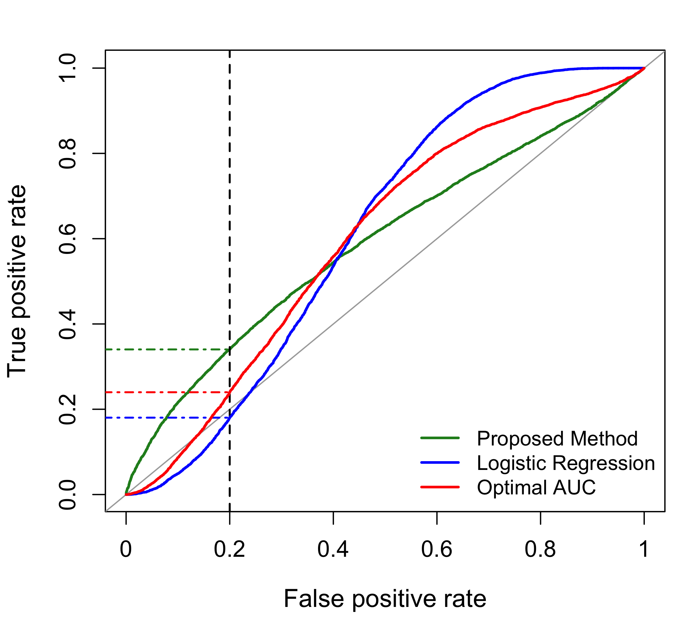
Figure 1 illustrates the importance of targeting the measure of interest in constructing biomarker combinations. In this example, combinations of three biomarkers are constructed by (i) maximizing the logistic likelihood, (ii) maximizing the AUC via the optAUC package in R (i.e., the method of Huang, Qin, and Fang (2011)), and (iii) maximizing the TPR for an FPR of 20% using the proposed method. The ROC curves for the three combinations differ markedly near the prespecified FPR of 20%. In particular, the TPRs at an FPR of 20% for the three combinations are 18.0%, 24.0%, and 34.0% for maximum likelihood, AUC optimization, and maximization of the TPR for a given FPR, respectively. This example highlights the utility of methods that target the TPR for a specific FPR as opposed to methods that target other measures.
3 Methodology
3.1 Description
Cases are denoted by the subscript and controls are denoted by the subscript . Let denote the vector of biomarkers for the case, and let denote the vector of biomarkers for the control.
We propose constructing a linear biomarker combination of the form for a -dimensional X by maximizing the TPR when the FPR is below some prespecified, clinically acceptable value . We define the true and false positive rates for a given X as a function of and :
Since the true and false positive rates for a given combination and threshold are invariant to scaling of the parameters , we must restrict to ensure identifiability. Specifically, we constrain as in Fong, Yin, and Huang (2016). For any fixed , we can consider
where This provides the optimal combination and threshold . We define to be an element of , where may be a set.
Of course, in practice, the true and false positive rates are unknown, so and cannot be computed. We can replace these unknowns by their empirical estimates,
where is the number of cases and is the number of controls, giving the total sample size . We can then define
where It is possible to conduct a grid search over to perform this constrained optimization, though this becomes computationally demanding when combining more than two or three biomarkers.
Since the objective function involves indicator functions, it is not a smooth function of the parameters and thus not amenable to derivative-based methods. However, smooth approximations to indicator functions have been used for AUC maximization (Ma and Huang, 2007; Fong, Yin, and Huang, 2016; Lin et al., 2011). One such smooth approximation is , where is the standard normal distribution function, and is a tuning parameter representing the trade-off between approximation accuracy and estimation feasibility such that tends to zero as the sample size grows (Lin et al., 2011). We can use this smooth approximation to implement the method described above, writing the smooth approximations to the empirical true and false positive rates as
Thus, we propose to compute
| (1) |
where Since both and are smooth functions, we can use gradient-based methods that incorporate the necessary constraints, e.g., Lagrange multipliers. In particular, can be obtained using existing software for constrained optimization of smooth functions, such as the Rsolnp package in R. An R package including code for our method based on Rsolnp, maxTPR, is available on CRAN. Other details related to implementation, including the choice of tuning parameter , are discussed below.
3.2 Asymptotic Properties
We present a theorem establishing that, under certain conditions, the combination obtained by optimizing the smooth approximation to the empirical TPR while constraining the smooth approximation to the empirical FPR has desirable operating characteristics. In particular, its FPR is bounded almost surely by the acceptable level in large samples. In addition, its TPR converges almost surely to the supremum of the TPR over the set where the FPR is constrained. We focus on the operating characteristics of since these are of primary interest to clinicians.
Rather than enforcing to be a strict maximizer, in the theoretical study below we allow it to be a near-maximizer of within in the sense that
where is a decreasing sequence of positive real numbers tending to zero. This provides some flexibility to accommodate situations in which a strict maximizer either does not exist or is numerically difficult to identify.
Before stating our key theorem, we give the following conditions.
-
(1)
Observations are randomly sampled conditional on disease status , and the group sizes tend to infinity proportionally, in the sense that and .
-
(2)
For each , observations , , are independent and identically distributed -dimensional random vectors with distribution function .
-
(3)
For each , no proper linear subspace is such that
-
(4)
For each , the distribution and quantile functions of given are globally Lipschitz continuous uniformly over such that .
-
(5)
The map is globally Lipschitz continuous over .
Theorem 1.
Under conditions (1)–(5), for every fixed , we have that
-
(a)
almost surely; and
-
(b)
tends to zero almost surely.
The proof of Theorem 1 is given in Appendix B. The proof relies on two lemmas, also in Appendix B. Lemma 1 demonstrates almost sure convergence to zero of the difference between the supremum of a function over a fixed set and the supremum of the function over a stochastic set that converges to the fixed set in an appropriate sense. Lemma 2 establishes the almost sure uniform convergence to zero of the difference between the FPR and the smooth approximation to the empirical FPR and the difference between the TPR and the smooth approximation to the empirical TPR. The proof of Theorem 1 demonstrates that Lemma 1 holds for the relevant function and sets, relying in part on the conclusions of Lemma 2. The conclusions of Lemmas 1 and 2 then demonstrate the claims of Theorem 1.
3.3 Implementation Details
Certain considerations must be addressed to implement the proposed method, including the choice of tuning parameter and starting values for the optimization routine. In using similar methods to maximize the AUC, Lin et al. (2011) proposed using , where is the sample standard error of . In simulations, we considered both and and found similar behavior for the convergence of the optimization routine. Thus, we use . We must also identify initial values for our procedure. As done in Fong, Yin, and Huang (2016), we use normalized estimates from robust logistic regression, which is described in greater detail below. Based on this initial value , we choose such that . In addition, we have also found that when is bounded by , the performance of the optimization routine can be poor. Thus, we introduce another tuning parameter, , which allows for a small amount of relaxation in the constraint on the smooth approximation to the empirical FPR, imposing instead Since the effective sample size for the smooth approximation to the empirical FPR is , we chose to scale with , and have found to work well.
Our method involves computing the gradient of the smooth approximations to the true and false positive rates defined above, which is fast regardless of the number of biomarkers involved. This is in contrast with methods that rely on brute force (e.g., grid search), which typically become computationally infeasible for combinations of more than two or three biomarkers. However, we note that for any method, the risk of overfitting is expected to grow as the number of biomarkers increases relative to the sample size. We emphasize that our method does not impose constraints on the distribution of the biomarkers that can be included, except for weak conditions that allow us to establish its large-sample properties.
4 Simulations
4.1 Bivariate Normal Biomarkers with Contamination
First, we considered bivariate normal biomarkers with contamination, similar to a scenario described by Croux and Haesbroeck (2003). In particular, we considered a setting where two biomarkers were independently normally distributed with mean zero and variance one. was then defined as where was distributed as a logistic random variable with location parameter zero and scale parameter one. Next, the sample was contaminated by a set of points with and . We consider simulations where the training set consisted of 800 or 1600 “typical” observations and 50 or 100, respectively, contaminating observations (this yielded a disease prevalence of approximately 47%). The test set consisted of “typical” observations and 62,500 contaminating observations. The maximum acceptable FPR, , was 0.2 or 0.3. We performed 1000 simulations.
We considered five approaches: (1) logistic regression, (2) the robust logistic regression method proposed by Bianco and Yohai (1996), (3) grid search, (4) the method proposed by Su and Liu (1993) and (5) the proposed method. As discussed above, the method proposed by Su and Liu (1993) yields a combination with maximum AUC when the biomarkers have a conditionally multivariate normal distribution. We did not consider the optimal AUC method proposed by Huang, Qin, and Fang (2011) as the implementation provided in R is too slow for use in simulations (and, as illustrated in Figure 1, may not yield a combination with optimal TPR). While the methods recently proposed by Yan et al. (2018) to optimize the partial AUC are compelling and may yield a combination with high TPR at the specified FPR value, implementation of their method, particularly the nonparametric kernel-based method, is non-trivial, and so is not included here. Finally, the method of Liu, Schisterman, and Zhu (2005), discussed above, may also yield a combination with high TPR at a particular FPR. However, given the shortcomings of this method described above (namely, that the range of FPRs over which the combination is optimal cannot be fixed in advanced and the biomarkers are assumed to have a conditionally multivariate normal distribution), we do not include this as a comparison method. Above all, none of these methods specifically target the TPR for a specified FPR which, as indicated by Figure 1, may lead to combinations with reduced TPR at the specified FPR.
We focused on evaluating the operating characteristics of the fitted combination rather than the biomarker coefficients as the former is typically of primary interest. In particular, we evaluated the TPR in the test data for FPR = in the test data. In other words, for each combination, the threshold used to calculate the TPR in the test data was chosen such that the FPR in the test data was equal to . Evaluating the TPR in this way puts the combinations on equal footing in terms of the FPR, and so allows a fair comparison of the TPR. We evaluated the FPR of the fitted combinations in the test data using the thresholds estimated in the training data, i.e., the th quantile of the fitted biomarker combination among controls in the training data. While we could have used the estimate of provided by our method in the evaluation, we found improved performance (that is, better control of the FPR) when re-estimating the threshold based on the fitted combination in the training data.
Table 1 summarizes the results. For both sample sizes and FPR thresholds, all methods adequately controlled the FPR, while for the TPR, the proposed method outperformed logistic regression, robust logistic regression, and the method of Su and Liu (1993). Furthermore, the results from the proposed method were comparable to those from the grid search, which may be regarded as a performance reference but is infeasible for more than two or three biomarkers.
| Measure | Method | |||||
|---|---|---|---|---|---|---|
| GLM | rGLM | Grid Search | Su & Liu | sTPR | ||
| 0.20 | ||||||
| 800 | TPR | 52.7 (15.9) | 55.8 (15.1) | 72.5 (0.9) | 53.6 (15.6) | 72.0 (4.5) |
| FPR | 20.4 (1.4) | 20.4 (1.4) | 20.6 (1.3) | 20.4 (1.4) | 20.4 (1.3) | |
| 1600 | TPR | 57.5 (13.2) | 60.0 (12.1) | 72.7 (0.5) | 58.3 (12.8) | 72.8 (0.5) |
| FPR | 20.3 (1.0) | 20.3 (1.0) | 20.4 (1.0) | 20.3 (1.0) | 20.3 (1.0) | |
| 0.30 | ||||||
| 800 | TPR | 68.5 (14.3) | 71.4 (13.6) | 86.0 (0.5) | 69.3 (13.9) | 86.0 (1.2) |
| FPR | 30.6 (1.8) | 30.6 (1.8) | 30.6 (1.8) | 30.6 (1.8) | 30.4 (1.8) | |
| 1600 | TPR | 74.0 (11.5) | 76.1 (10.3) | 86.1 (0.3) | 74.7 (11.1) | 86.1 (0.3) |
| FPR | 30.4 (1.3) | 30.3 (1.3) | 30.4 (1.3) | 30.4 (1.3) | 30.2 (1.3) | |
4.2 Conditionally Multivariate Lognormal Biomarkers
We also considered simulations with conditionally multivariate lognormal biomarkers (Mishra, 2019). In particular, we considered three biomarkers . Among controls, and had a bivariate normal distribution with and . Among cases, and had a bivariate normal distribution with and . The third biomarker, was simulated from an independent lognormal distribution with and among both cases and controls. Given the performance of the method of Su and Liu (1993) and the performance of the proposed method relative to grid search observed above (and the computational challenges of implementing grid search for three biomarkers), we considered three methods here: (1) logistic regression, (2) robust logistic regression, and (3) the proposed method. Although neither logistic regression nor robust logistic regression performed particularly well in the simulations in Section 4.1, these methods represent the most commonly used approach for constructing biomarker combinations and the method used to provide starting values for the proposed method, respectively. Thus, it was important to include them here.
The maximum acceptable FPR, , was 0.2 and 1000 simulations were performed. The training data consisted of either 400 cases and 400 controls, or 800 cases and 800 controls. The test data consisted of observations. The TPR and FPR were evaluated as described above. We present the results in Table 2. All three methods did well in controlling the FPR at the specified value. Furthermore, the proposed method substantially outperformed logistic regression and robust logistic regression: the mean TPR based on the proposed method was at least 20% larger than the mean TPRs from logistic regression and robust logistic regression.
| Measure | Method | |||
|---|---|---|---|---|
| GLM | rGLM | sTPR | ||
| 800 | TPR | 34.1 (6.0) | 34.1 (6.0) | 41.5 (5.7) |
| FPR | 30.3 (2.3) | 30.3 (2.3) | 31.2 (2.4) | |
| 1600 | TPR | 34.7 (4.2) | 34.7 (4.2) | 41.9 (4.9) |
| FPR | 30.2 (1.6) | 30.2 (1.6) | 30.7 (1.7) | |
4.3 Bivariate Normal Biomarkers and Bivariate Normal Mixture Biomarkers
The above simulations demonstrate superiority of our approach relative to alternative methods in particular scenarios. We conducted further simulations to demonstrate the feasibility of our approach in other settings (for instance, small sample size, small and large prevalence, and low FPR cutoffs) relative to logistic regression and robust logistic regression.
We considered simulations with and without outliers in the data-generating distribution, and simulated data under a model similar to that used by Fong, Yin, and Huang (2016). We considered two biomarkers and constructed as
where was a Bernoulli random variable with success probability when outliers were simulated and otherwise, and and were independent bivariate normal random variables with mean zero and respective covariance matrices
was then simulated as a Bernoulli random variable with success probability . We considered two functions: and a piecewise logistic function,
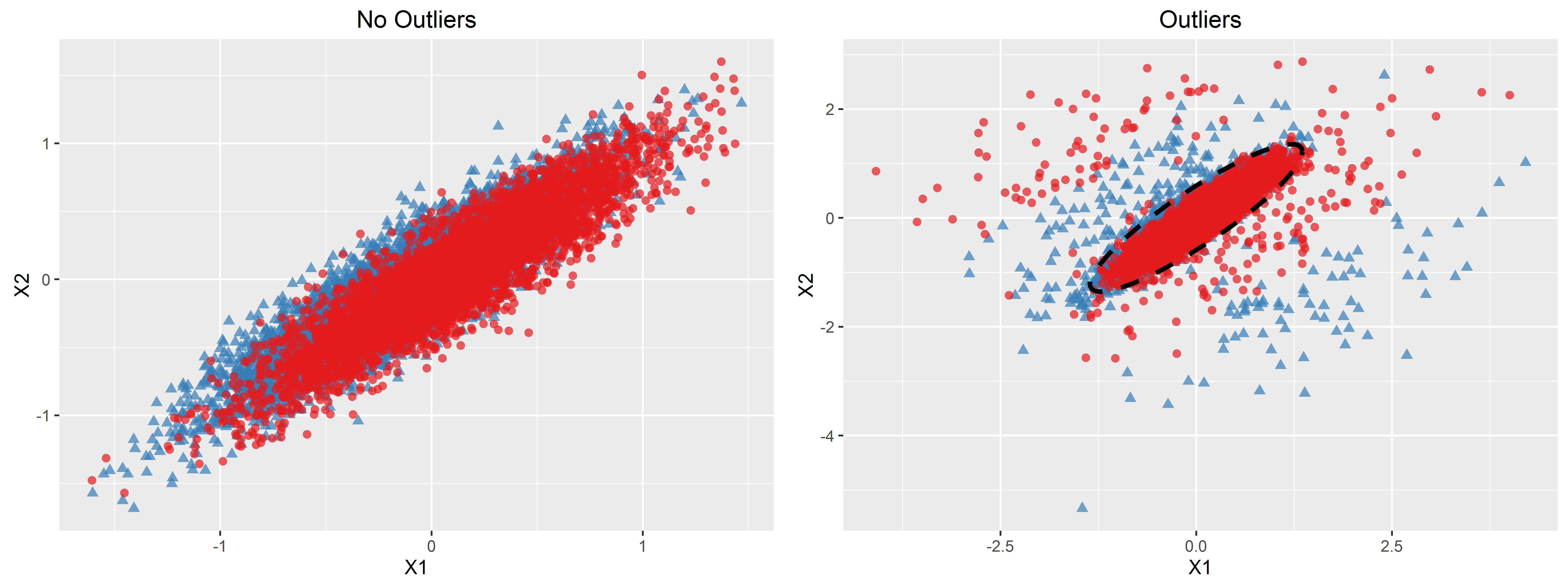
We varied to reflect varying prevalences, with a prevalence of approximately 50–60% for 0, 16–18% for 0, and 77–82% for 0. We considered 0.05, 0.1, and 0.2. A plot illustrating the data-generating distribution with and 0, with and without outliers, is given in Appendix D.
The training data consisted of 200, 400, or 800 observations while the test set included observations. The TPR and FPR were evaluated as described above. The results are presented in Appendix C. When no outliers were present, the proposed method was comparable to logistic regression and robust logistic regression in terms of both the TPR and FPR. In the presence of outliers, robust logistic regression tended to provide combinations with higher TPRs than did logistic regression, and the TPRs of the combinations provided by the proposed method tended to be comparable to or somewhat better than the results from robust logistic regression. In all scenarios, all three methods controlled the FPR, particularly as sample size increased. In addition to demonstrating feasibility of our approach, these simulations highlight the fact that logistic regression is relatively robust to violations of the linear-logistic model (e.g., nonlinear biomarker combinations and deviations from the logit link).
4.4 Convergence
In most simulation settings, convergence of the proposed method was achieved in more than of simulations. For some of the more extreme outlier scenarios considered in Section 4.3, convergence failed in up to of simulations.
5 Application to Diabetes Data
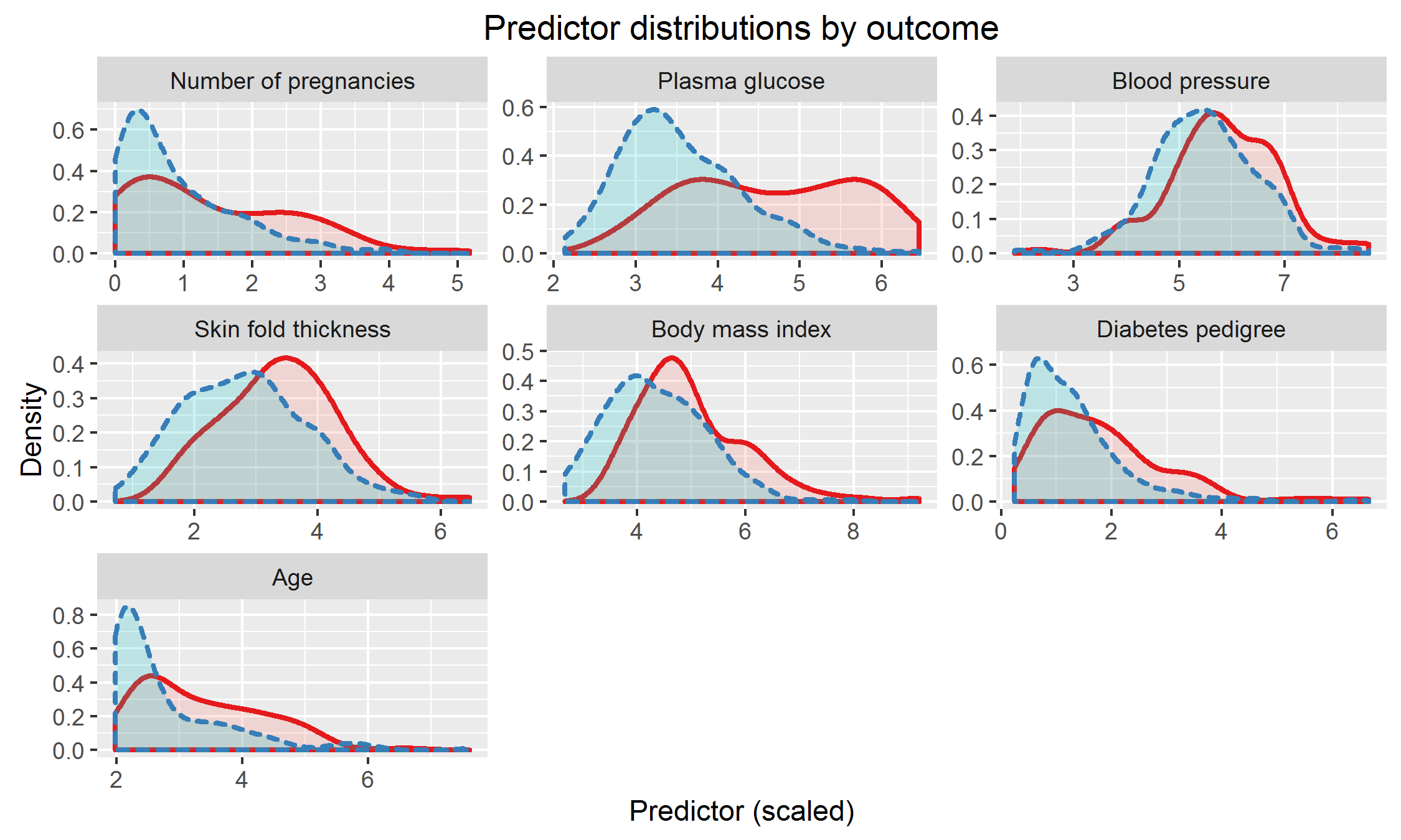
We applied the method we have developed to a study of diabetes in women with Pima Indian heritage (Smith et al., 1988). We considered seven predictors measured in this study: number of pregnancies, plasma glucose concentration, diastolic blood pressure, triceps skin fold thickness, body mass index, age, and diabetes pedigree function (a measure of family history of diabetes (Smith et al., 1988)). We used 332 observations as training data and reserved the remaining 200 observations for testing. The training and test datasets had 109 and 68 diabetes cases, respectively. We scaled the variables to have equal variance. The distribution of predictors is depicted in Appendix E. The combinations were fitted using the training data and evaluated using the test data. We fixed the acceptable FPR at . We used logistic regression, robust logistic regression, and the proposed method to construct the combinations, giving the results in Table 3, where the fitted combinations from logistic regression and robust logistic regression have been normalized to aid in comparison.
| Predictor | GLM | rGLM | sTPR |
|---|---|---|---|
| Number of pregnancies | 0.321 | 0.320 | 0.403 |
| Plasma glucose | 0.793 | 0.792 | 0.627 |
| Blood pressure | 0.077 | 0.073 | 0.026 |
| Skin fold thickness | 0.089 | 0.090 | 0.146 |
| Body mass index | 0.399 | 0.400 | 0.609 |
| Diabetes pedigree | 0.280 | 0.281 | 0.191 |
| Age | 0.133 | 0.134 | 0.123 |
Using thresholds based on an FPR of 10% in the test data, the estimated TPR in the test data was 54.4% for both logistic regression and robust logistic regression, and 55.9% for the proposed method. The estimated FPR in the test data using thresholds corresponding to an FPR of 10% in the training data was 18.2% for both logistic regression and robust logistic regression and 26.5% for the proposed method. The fact that these FPRs exceeded the target value for all three methods indicates potentially important differences in the controls between the training and test data.
6 Discussion
We have proposed a distribution-free method for constructing linear biomarker combinations by maximizing a smooth approximation to the TPR while constraining a smooth approximation to the FPR. Ours is the first distribution-free approach targeting the TPR for a specified FPR that can be used with more than two or three biomarkers. While we do not expect our method to outperform every other approach in every dataset, we have demonstrated broad feasibility of our method and, importantly, we have identified scenarios where the performance of our method is superior to alternative approaches.
The proposed method could be adapted to minimize the FPR while controlling the TPR to be above some acceptable level. Since the TPR and FPR condition on disease status, the proposed method can be used with case-control data. For case-control data matched on a covariate, however, it becomes necessary to consider the covariate-adjusted ROC curve and corresponding covariate-adjusted summaries, and thus the methods presented here are not immediately applicable (Janes and Pepe, 2008).
As our smooth approximation function is non-convex, the choice of starting values should be considered further. Extensions of convex methods, such as the ramp function method proposed by Fong, Yin, and Huang (2016) for the AUC, could also be considered. The idea of partitioning the search space, proposed by Yan et al. (2018), may also be useful. Further research could investigate methods for evaluating the true and false positive rates of biomarker combinations after estimation, for example, sample-splitting, bootstrapping, or -fold cross-validation.
7 Software
An R package containing code to implement the proposed method, maxTPR, is publicly available via CRAN.
Funding
This work was supported by the National Institutes of Health [F31 DK108356, R01 CA152089, and R01 HL085757]; and the University of Washington Department of Biostatistics Career Development Fund [to M.C.]. The opinions, results, and conclusions reported in this article are those of the authors and are independent of the funding sources.
Appendix A
Proposition 1.
If the biomarkers are conditionally multivariate normal with proportional covariance matrices given , that is,
then the optimal biomarker combination in the sense of the ROC curve is of the form
for some vector .
Proof.
It is known that the optimal combination of in terms of the ROC curve is the likelihood ratio, , or any monotone increasing function thereof (McIntosh and Pepe, 2002). Let . Without loss of generality, let and . Then
Denote the entries of by
Then, we can write that
as claimed, where
∎
Appendix B
The proof of Theorem 1 relies on Lemmas 1 and 2, which are stated and proved below.
Lemma 1.
Say that a bounded function and possibly random sets are given, and let be a decreasing sequence of positive real numbers tending to zero. For each , suppose that and are near-maximizers of over and , respectively, in the sense that and . Further, define
where is the Euclidean distance in . If and tend to zero almost surely, and is globally Lipschitz continuous, then tends to zero almost surely. In particular, this implies that
almost surely.
Proof.
Say that both and tend to zero almost surely, and denote by the Lipschitz constant of . Suppose that for some we have that
We will show that this leads to a contradiction, and thus that it must be true that
for each , thus establishing the desired result.
On a set of probability one, there exists an such that, for each , there exists and satisfying and . Then, on this same set, for , and , so that and in particular. Since and , it must also be true that and . This then implies that for all on a set of probability one. Since tends to zero deterministically, this yields the sought contradiction.
To establish the last portion of the Lemma, we simply use the first part along with the fact that
∎
Lemma 2.
Under conditions (1)–(5), we have that
almost surely as tends to , where .
Proof.
We prove the claim for the false positive rate (FPR); the proof for the true positive rate (TPR) is analogous. We can write
First, we consider . We can write this as
The class of functions is a Vapnik–Chervonenkis (VC) class. Since is monotone for each , the class of functions is also VC (Kosorok, 2008; van der Vaart, 1998; van der Vaart and Wellner, 2000). Since the constant 1 is an applicable envelope function for this class, is –Glivenko-Cantelli, giving that (Kosorok, 2008; van der Vaart and Wellner, 2000)
almost surely.
Next, we consider . We can write this as
For a general random variable with distribution function that is Lipschitz continuous, say with constant , we can write
with . Using integration by parts and Lemma 2.1 from Winter (1979), this becomes
and so, we find that
Since tends to zero as tends to infinity, this implies that
We now return to and consider the case , so that Let and . Then, we have that , where and . We find that
for any . Since , we can write
implying, in view of condition (4) and the results above, that
The result for can be proved analogously.
Combining these results, we conclude that tends to zero almost surely, as claimed. ∎
Proof of Theorem 1.
First, we show that almost surely. We can write
As such, it follows that
in view of Lemma 2, thereby establishing the first part of the theorem.
Let be fixed. We now establish that
almost surely. For convenience, denote by . Consider the function defined pointwise as , and set and for each . We verify that the conditions of Lemma 1 hold for these particular choices. We have that is a bounded function. We must show and tend to zero almost surely, where
and is the Euclidean distance in . We consider first. Denote by the conditional distribution function of given . By assumption, the corresponding conditional quantile function, denoted by , is uniformly Lipschitz continuous over , say with constant independent of . Suppose that, for some , . Because it is true that
then , giving and for each .
For any given , write , giving . If , note also that and set . Otherwise, find such that , namely by taking . Defining , observe that
Thus, for each , it is true that and therefore . As such, if for some , then for . This implies that
by Lemma 2. Thus, tends to zero almost surely since, for each ,
Using similar arguments, we may show that also tends to zero almost surely.
The fact that and tend to zero almost surely implies, in view of Lemma 1, that we have that tends to zero almost surely. Combining this with an application of Lemma 2, we have that
almost surely. Since and, by Lemma 2, tends to zero almost surely, tends to zero almost surely. In addition, since is a near-maximizer of , , giving
almost surely, completing the proof. ∎
Appendix C: Simulation results for data with outliers
Note: When simulating with outliers, the true biomarker combination was occasionally so large that it returned a non-value for the outcome ; for example, with , this occurs in R when . These observations had to be removed from the simulated dataset, though this affected an extremely small fraction of observations.
| Outliers | Measure | Method | |||
|---|---|---|---|---|---|
| GLM | rGLM | sTPR | |||
| 0.05 | |||||
| Yes | 200 | TPR | 12.2 (2.1) | 13.6 (2.6) | 13.4 (2.7) |
| FPR | 5.7 (2.2) | 5.9 (2.3) | 6.4 (2.4) | ||
| 400 | TPR | 12.1 (1.7) | 14.1 (2.3) | 13.9 (2.4) | |
| FPR | 5.4 (1.6) | 5.4 (1.6) | 5.9 (1.7) | ||
| 800 | TPR | 11.8 (1.2) | 14.4 (2.2) | 14.4 (2.3) | |
| FPR | 5.1 (1.1) | 5.2 (1.1) | 5.5 (1.2) | ||
| No | 200 | TPR | 18.3 (0.6) | 18.3 (0.6) | 17.8 (1.8) |
| FPR | 5.5 (2.2) | 5.5 (2.2) | 6.2 (2.4) | ||
| 400 | TPR | 18.5 (0.3) | 18.5 (0.3) | 18.1 (1.6) | |
| FPR | 5.3 (1.5) | 5.3 (1.5) | 5.7 (1.6) | ||
| 800 | TPR | 18.6 (0.2) | 18.6 (0.2) | 18.4 (1.2) | |
| FPR | 5.2 (1.1) | 5.2 (1.1) | 5.5 (1.2) | ||
| 0.10 | |||||
| Yes | 200 | TPR | 22.5 (3.8) | 24.6 (4.3) | 24.6 (4.2) |
| FPR | 10.9 (3.1) | 11.1 (3.0) | 11.7 (3.2) | ||
| 400 | TPR | 21.8 (2.8) | 25.1 (4.0) | 25.2 (4.0) | |
| FPR | 10.4 (2.0) | 10.5 (2.1) | 11.0 (2.1) | ||
| 800 | TPR | 21.4 (2.0) | 25.7 (3.6) | 25.8 (3.6) | |
| FPR | 10.1 (1.5) | 10.1 (1.5) | 10.5 (1.5) | ||
| No | 200 | TPR | 29.4 (0.8) | 29.5 (0.8) | 28.9 (2.2) |
| FPR | 10.5 (3.1) | 10.5 (3.1) | 11.4 (3.2) | ||
| 400 | TPR | 29.8 (0.4) | 29.8 (0.4) | 29.5 (1.3) | |
| FPR | 10.4 (2.1) | 10.4 (2.1) | 10.9 (2.2) | ||
| 800 | TPR | 29.9 (0.2) | 29.9 (0.2) | 29.7 (1.5) | |
| FPR | 10.2 (1.5) | 10.2 (1.5) | 10.6 (1.5) | ||
| 0.20 | |||||
| Yes | 200 | TPR | 38.0 (5.1) | 40.8 (5.8) | 41.0 (5.7) |
| FPR | 20.9 (4.0) | 21.1 (4.0) | 21.8 (4.0) | ||
| 400 | TPR | 37.4 (3.9) | 41.7 (5.3) | 41.9 (5.2) | |
| FPR | 20.5 (2.8) | 20.6 (2.9) | 21.1 (2.9) | ||
| 800 | TPR | 36.9 (2.9) | 42.4 (4.6) | 43.0 (4.4) | |
| FPR | 20.2 (2.0) | 20.4 (2.0) | 20.7 (2.0) | ||
| No | 200 | TPR | 46.1 (0.9) | 46.1 (0.9) | 45.7 (1.5) |
| FPR | 20.7 (4.1) | 20.8 (4.1) | 21.7 (4.2) | ||
| 400 | TPR | 46.4 (0.5) | 46.4 (0.5) | 46.2 (0.8) | |
| FPR | 20.3 (2.8) | 20.3 (2.8) | 21.0 (2.8) | ||
| 800 | TPR | 46.5 (0.2) | 46.5 (0.3) | 46.4 (0.6) | |
| FPR | 20.1 (2.0) | 20.1 (2.0) | 20.5 (2.0) | ||
| Outliers | Measure | Method | |||
|---|---|---|---|---|---|
| GLM | rGLM | sTPR | |||
| 0.05 | |||||
| Yes | 200 | TPR | 20.2 (7.3) | 26.4 (9.1) | 27.7 (9.2) |
| FPR | 5.9 (2.6) | 6.0 (2.6) | 6.5 (2.8) | ||
| 400 | TPR | 19.0 (5.9) | 27.6 (8.5) | 29.3 (8.2) | |
| FPR | 5.5 (1.8) | 5.5 (1.7) | 5.8 (1.8) | ||
| 800 | TPR | 17.9 (4.1) | 29.4 (7.5) | 30.8 (7.3) | |
| FPR | 5.3 (1.3) | 5.3 (1.2) | 5.5 (1.3) | ||
| No | 200 | TPR | 37.9 (1.7) | 37.8 (1.9) | 37.5 (3.1) |
| FPR | 5.8 (2.7) | 5.7 (2.7) | 6.5 (2.9) | ||
| 400 | TPR | 38.6 (0.9) | 38.5 (1.0) | 38.3 (2.1) | |
| FPR | 5.3 (1.8) | 5.3 (1.8) | 5.8 (1.8) | ||
| 800 | TPR | 38.9 (0.4) | 38.9 (0.5) | 38.6 (2.2) | |
| FPR | 5.2 (1.3) | 5.2 (1.3) | 5.5 (1.3) | ||
| 0.10 | |||||
| Yes | 200 | TPR | 31.1 (8.9) | 37.4 (10.8) | 39.3 (11.0) |
| FPR | 11.0 (3.5) | 11.3 (3.6) | 12.0 (3.6) | ||
| 400 | TPR | 30.3 (7.1) | 39.9 (9.8) | 41.5 (9.6) | |
| FPR | 10.5 (2.5) | 10.7 (2.4) | 11.0 (2.5) | ||
| 800 | TPR | 28.9 (5.0) | 41.1 (8.9) | 43.1 (8.6) | |
| FPR | 10.1 (1.7) | 10.3 (1.7) | 10.6 (1.8) | ||
| No | 200 | TPR | 48.2 (1.8) | 48.0 (1.9) | 48.2 (2.0) |
| FPR | 10.9 (3.5) | 10.9 (3.5) | 11.7 (3.6) | ||
| 400 | TPR | 48.8 (0.9) | 48.7 (1.0) | 48.7 (1.1) | |
| FPR | 10.4 (2.4) | 10.4 (2.4) | 10.9 (2.5) | ||
| 800 | TPR | 49.2 (0.4) | 49.1 (0.5) | 49.0 (0.6) | |
| FPR | 10.2 (1.7) | 10.2 (1.7) | 10.7 (1.8) | ||
| 0.20 | |||||
| Yes | 200 | TPR | 45.0 (8.1) | 50.4 (9.8) | 51.9 (9.7) |
| FPR | 21.2 (4.6) | 21.5 (4.7) | 22.0 (4.8) | ||
| 400 | TPR | 44.4 (6.3) | 52.8 (8.6) | 54.0 (8.5) | |
| FPR | 20.4 (3.2) | 20.8 (3.3) | 21.2 (3.4) | ||
| 800 | TPR | 44.1 (4.8) | 54.8 (7.3) | 56.5 (6.6) | |
| FPR | 20.2 (2.3) | 20.3 (2.3) | 20.7 (2.3) | ||
| No | 200 | TPR | 59.5 (1.3) | 59.4 (1.4) | 59.3 (1.8) |
| FPR | 21.1 (4.6) | 21.1 (4.6) | 22.1 (4.7) | ||
| 400 | TPR | 60.0 (0.6) | 59.9 (0.7) | 59.8 (0.9) | |
| FPR | 20.5 (3.4) | 20.6 (3.4) | 21.2 (3.4) | ||
| 800 | TPR | 60.2 (0.4) | 60.1 (0.4) | 60.1 (0.5) | |
| FPR | 20.3 (2.2) | 20.3 (2.2) | 20.7 (2.3) | ||
| Outliers | Measure | Method | |||
|---|---|---|---|---|---|
| GLM | rGLM | sTPR | |||
| 0.05 | |||||
| Yes | 200 | TPR | 13.0 (2.8) | 13.4 (3.4) | 13.5 (3.4) |
| FPR | 5.3 (1.7) | 5.4 (1.7) | 5.7 (1.8) | ||
| 400 | TPR | 12.7 (1.9) | 13.4 (2.7) | 13.6 (2.9) | |
| FPR | 5.2 (1.2) | 5.2 (1.2) | 5.4 (1.2) | ||
| 800 | TPR | 12.5 (1.3) | 13.2 (2.1) | 13.6 (2.5) | |
| FPR | 5.1 (0.8) | 5.2 (0.8) | 5.2 (0.9) | ||
| No | 200 | TPR | 18.1 (1.0) | 18.1 (1.1) | 17.5 (2.2) |
| FPR | 5.5 (1.8) | 5.5 (1.8) | 5.9 (1.8) | ||
| 400 | TPR | 18.5 (0.6) | 18.5 (0.6) | 18.2 (1.6) | |
| FPR | 5.1 (1.2) | 5.2 (1.2) | 5.4 (1.3) | ||
| 800 | TPR | 18.7 (0.3) | 18.7 (0.3) | 18.5 (1.1) | |
| FPR | 5.1 (0.9) | 5.1 (0.9) | 5.3 (0.9) | ||
| 0.10 | |||||
| Yes | 200 | TPR | 22.1 (4.5) | 22.7 (5.3) | 23.1 (5.3) |
| FPR | 10.4 (2.4) | 10.5 (2.4) | 10.8 (2.4) | ||
| 400 | TPR | 21.9 (3.6) | 22.8 (4.7) | 23.4 (4.8) | |
| FPR | 10.1 (1.7) | 10.2 (1.7) | 10.4 (1.8) | ||
| 800 | TPR | 21.4 (2.3) | 22.3 (3.4) | 23.3 (4.3) | |
| FPR | 10.1 (1.2) | 10.1 (1.2) | 10.3 (1.2) | ||
| No | 200 | TPR | 29.5 (1.3) | 29.4 (1.3) | 28.8 (2.5) |
| FPR | 10.3 (2.3) | 10.4 (2.3) | 10.9 (2.3) | ||
| 400 | TPR | 29.8 (0.7) | 29.8 (0.7) | 29.5 (1.5) | |
| FPR | 10.2 (1.7) | 10.2 (1.7) | 10.6 (1.7) | ||
| 800 | TPR | 30.1 (0.4) | 30.1 (0.4) | 29.8 (1.1) | |
| FPR | 10.1 (1.1) | 10.1 (1.1) | 10.3 (1.1) | ||
| 0.20 | |||||
| Yes | 200 | TPR | 36.4 (6.6) | 37.2 (7.8) | 38.1 (7.4) |
| FPR | 20.5 (3.2) | 20.6 (3.1) | 21.0 (3.2) | ||
| 400 | TPR | 36.2 (4.7) | 37.3 (6.2) | 38.5 (6.4) | |
| FPR | 20.1 (2.2) | 20.2 (2.3) | 20.4 (2.2) | ||
| 800 | TPR | 35.7 (3.0) | 37.0 (4.6) | 38.8 (5.7) | |
| FPR | 20.2 (1.5) | 20.2 (1.5) | 20.4 (1.5) | ||
| No | 200 | TPR | 46.1 (1.7) | 46.1 (1.7) | 45.5 (2.6) |
| FPR | 20.4 (3.1) | 20.5 (3.2) | 21.0 (3.2) | ||
| 400 | TPR | 46.7 (0.8) | 46.7 (0.8) | 46.4 (1.3) | |
| FPR | 20.1 (2.1) | 20.2 (2.1) | 20.5 (2.1) | ||
| 800 | TPR | 47.0 (0.4) | 47.0 (0.4) | 46.8 (0.7) | |
| FPR | 20.0 (1.6) | 20.0 (1.6) | 20.2 (1.6) | ||
| Outliers | Measure | Method | |||
|---|---|---|---|---|---|
| GLM | rGLM | sTPR | |||
| 0.05 | |||||
| Yes | 200 | TPR | 8.4 (1.2) | 8.4 (1.4) | 8.2 (1.8) |
| FPR | 7.3 (4.0) | 6.9 (3.9) | 7.7 (4.6) | ||
| 400 | TPR | 8.6 (0.9) | 8.5 (1.1) | 8.3 (1.6) | |
| FPR | 6.3 (2.7) | 6.3 (2.7) | 6.7 (2.9) | ||
| 800 | TPR | 8.7 (0.6) | 8.6 (0.7) | 8.5 (1.5) | |
| FPR | 5.8 (1.8) | 5.8 (1.8) | 6.1 (2.0) | ||
| No | 200 | TPR | 18.7 (1.0) | 18.7 (1.0) | 17.2 (3.5) |
| FPR | 6.3 (4.1) | 6.1 (4.0) | 7.4 (4.5) | ||
| 400 | TPR | 19.0 (0.5) | 19.0 (0.6) | 17.9 (2.9) | |
| FPR | 5.7 (2.7) | 5.6 (2.7) | 6.4 (3.0) | ||
| 800 | TPR | 19.2 (0.3) | 19.2 (0.3) | 18.3 (2.9) | |
| FPR | 5.3 (1.9) | 5.3 (1.9) | 5.9 (2.0) | ||
| 0.10 | |||||
| Yes | 200 | TPR | 18.6 (3.9) | 19.1 (4.7) | 19.4 (4.8) |
| FPR | 12.4 (5.1) | 12.4 (5.0) | 13.5 (5.4) | ||
| 400 | TPR | 18.6 (2.5) | 19.2 (3.5) | 19.8 (3.8) | |
| FPR | 11.1 (3.4) | 11.1 (3.5) | 12.0 (3.7) | ||
| 800 | TPR | 18.4 (1.4) | 19.2 (2.6) | 19.8 (3.4) | |
| FPR | 10.8 (2.6) | 10.8 (2.6) | 11.3 (2.7) | ||
| No | 200 | TPR | 29.9 (1.3) | 29.9 (1.3) | 28.7 (3.6) |
| FPR | 11.7 (5.2) | 11.5 (5.2) | 13.1 (5.6) | ||
| 400 | TPR | 30.4 (0.6) | 30.3 (0.7) | 29.4 (3.4) | |
| FPR | 10.7 (3.6) | 10.6 (3.6) | 11.7 (3.8) | ||
| 800 | TPR | 30.6 (0.3) | 30.6 (0.3) | 30.2 (2.0) | |
| FPR | 10.4 (2.5) | 10.4 (2.5) | 11.1 (2.5) | ||
| 0.20 | |||||
| Yes | 200 | TPR | 34.2 (6.4) | 34.9 (7.7) | 35.9 (7.1) |
| FPR | 22.5 (6.5) | 22.7 (6.3) | 24.0 (6.7) | ||
| 400 | TPR | 34.2 (4.3) | 35.0 (5.6) | 36.3 (5.9) | |
| FPR | 21.4 (4.7) | 21.5 (4.7) | 22.4 (4.8) | ||
| 800 | TPR | 33.9 (2.8) | 35.0 (4.4) | 36.2 (5.0) | |
| FPR | 20.6 (3.3) | 20.7 (3.3) | 21.3 (3.4) | ||
| No | 200 | TPR | 46.4 (1.6) | 46.4 (1.6) | 45.6 (3.3) |
| FPR | 22.2 (7.0) | 22.0 (7.0) | 23.9 (7.1) | ||
| 400 | TPR | 47.0 (0.8) | 47.0 (0.8) | 46.5 (2.2) | |
| FPR | 20.8 (5.0) | 20.7 (4.9) | 22.0 (5.0) | ||
| 800 | TPR | 47.2 (0.4) | 47.2 (0.4) | 46.9 (1.9) | |
| FPR | 20.6 (3.4) | 20.6 (3.4) | 21.4 (3.5) | ||
| Outliers | Measure | Method | |||
|---|---|---|---|---|---|
| GLM | rGLM | sTPR | |||
| 0.05 | |||||
| Yes | 200 | TPR | 7.1 (1.1) | 7.1 (1.1) | 7.1 (1.1) |
| FPR | 5.7 (1.8) | 5.7 (1.8) | 5.9 (1.9) | ||
| 400 | TPR | 7.4 (1.0) | 7.3 (0.9) | 7.3 (1.0) | |
| FPR | 5.3 (1.2) | 5.4 (1.2) | 5.5 (1.2) | ||
| 800 | TPR | 7.6 (0.8) | 7.5 (0.8) | 7.5 (0.9) | |
| FPR | 5.1 (0.8) | 5.2 (0.8) | 5.2 (0.9) | ||
| No | 200 | TPR | 7.3 (1.4) | 7.3 (1.4) | 7.2 (1.4) |
| FPR | 5.5 (1.7) | 5.6 (1.7) | 5.9 (1.8) | ||
| 400 | TPR | 7.8 (0.9) | 7.8 (1.0) | 7.7 (1.1) | |
| FPR | 5.2 (1.2) | 5.2 (1.1) | 5.4 (1.2) | ||
| 800 | TPR | 8.1 (0.4) | 8.1 (0.4) | 8.0 (0.7) | |
| FPR | 5.1 (0.9) | 5.1 (0.9) | 5.2 (0.9) | ||
| 0.10 | |||||
| Yes | 200 | TPR | 12.4 (2.0) | 12.3 (2.0) | 12.4 (2.0) |
| FPR | 10.6 (2.3) | 10.6 (2.3) | 10.9 (2.4) | ||
| 400 | TPR | 12.6 (1.7) | 12.4 (1.7) | 12.6 (1.8) | |
| FPR | 10.4 (1.7) | 10.4 (1.7) | 10.6 (1.7) | ||
| 800 | TPR | 12.8 (1.5) | 12.5 (1.5) | 12.7 (1.6) | |
| FPR | 10.2 (1.2) | 10.2 (1.1) | 10.3 (1.2) | ||
| No | 200 | TPR | 13.9 (2.2) | 13.9 (2.2) | 13.6 (2.3) |
| FPR | 10.7 (2.3) | 10.8 (2.3) | 11.2 (2.4) | ||
| 400 | TPR | 14.5 (1.5) | 14.5 (1.5) | 14.4 (1.6) | |
| FPR | 10.2 (1.6) | 10.2 (1.6) | 10.5 (1.6) | ||
| 800 | TPR | 15.0 (0.8) | 15.0 (0.8) | 14.9 (1.0) | |
| FPR | 10.2 (1.2) | 10.2 (1.2) | 10.4 (1.2) | ||
| 0.20 | |||||
| Yes | 200 | TPR | 22.4 (3.6) | 22.2 (3.7) | 22.5 (3.7) |
| FPR | 20.9 (3.1) | 20.9 (3.2) | 21.3 (3.2) | ||
| 400 | TPR | 22.6 (3.3) | 22.3 (3.3) | 22.7 (3.3) | |
| FPR | 20.6 (2.2) | 20.6 (2.2) | 20.9 (2.2) | ||
| 800 | TPR | 22.8 (2.7) | 22.3 (2.8) | 22.8 (2.8) | |
| FPR | 20.2 (1.5) | 20.2 (1.6) | 20.4 (1.6) | ||
| No | 200 | TPR | 25.8 (3.5) | 25.7 (3.5) | 25.5 (3.6) |
| FPR | 20.9 (3.1) | 20.9 (3.1) | 21.4 (3.1) | ||
| 400 | TPR | 26.9 (2.3) | 26.9 (2.3) | 26.8 (2.3) | |
| FPR | 20.5 (2.1) | 20.5 (2.1) | 20.8 (2.1) | ||
| 800 | TPR | 27.7 (1.1) | 27.7 (1.1) | 27.5 (1.3) | |
| FPR | 20.3 (1.6) | 20.3 (1.6) | 20.5 (1.6) | ||
| Outliers | Measure | Method | |||
|---|---|---|---|---|---|
| GLM | rGLM | sTPR | |||
| 0.05 | |||||
| Yes | 200 | TPR | 23.0 (8.6) | 30.5 (10.9) | 31.9 (10.8) |
| FPR | 6.4 (3.3) | 6.3 (3.4) | 6.8 (3.7) | ||
| Yes | 400 | TPR | 21.5 (6.9) | 31.8 (10.5) | 33.5 (10.1) |
| FPR | 5.8 (2.3) | 5.8 (2.4) | 6.2 (2.6) | ||
| Yes | 800 | TPR | 20.0 (4.4) | 34.6 (9.2) | 35.8 (8.5) |
| FPR | 5.4 (1.6) | 5.3 (1.6) | 5.7 (1.7) | ||
| No | 200 | TPR | 49.7 (1.5) | 49.5 (1.7) | 48.6 (4.4) |
| FPR | 6.0 (3.5) | 5.9 (3.5) | 6.8 (3.7) | ||
| No | 400 | TPR | 50.3 (0.7) | 50.1 (0.8) | 49.7 (2.3) |
| FPR | 5.5 (2.5) | 5.4 (2.5) | 6.1 (2.6) | ||
| No | 800 | TPR | 50.5 (0.4) | 50.5 (0.5) | 50.1 (2.0) |
| FPR | 5.2 (1.6) | 5.2 (1.6) | 5.6 (1.7) | ||
| 0.10 | |||||
| Yes | 200 | TPR | 37.3 (11.0) | 45.7 (13.7) | 48.4 (13.2) |
| FPR | 11.5 (4.5) | 11.6 (4.5) | 12.4 (4.6) | ||
| Yes | 400 | TPR | 35.2 (8.5) | 47.5 (12.9) | 50.6 (12.1) |
| FPR | 10.8 (3.1) | 10.9 (3.2) | 11.4 (3.3) | ||
| Yes | 800 | TPR | 34.5 (6.6) | 51.3 (10.7) | 53.6 (10.2) |
| FPR | 10.4 (2.2) | 10.4 (2.2) | 10.8 (2.3) | ||
| No | 200 | TPR | 61.3 (1.4) | 61.1 (1.6) | 60.7 (3.2) |
| FPR | 10.9 (4.5) | 10.9 (4.5) | 12.1 (4.7) | ||
| No | 400 | TPR | 61.8 (0.7) | 61.6 (0.8) | 61.4 (1.2) |
| FPR | 10.6 (3.2) | 10.6 (3.2) | 11.4 (3.3) | ||
| No | 800 | TPR | 62.0 (0.4) | 62.0 (0.4) | 61.8 (0.8) |
| FPR | 10.3 (2.3) | 10.3 (2.3) | 10.9 (2.4) | ||
| 0.20 | |||||
| Yes | 200 | TPR | 53.2 (10.6) | 60.9 (13.0) | 64.2 (12.3) |
| FPR | 21.2 (5.9) | 21.8 (6.0) | 22.8 (6.0) | ||
| Yes | 400 | TPR | 52.0 (8.5) | 63.5 (11.8) | 65.4 (11.3) |
| FPR | 20.7 (4.1) | 21.1 (4.2) | 21.7 (4.1) | ||
| Yes | 800 | TPR | 51.1 (6.0) | 66.3 (9.7) | 68.6 (8.2) |
| FPR | 20.4 (3.0) | 20.6 (3.0) | 21.1 (3.0) | ||
| No | 200 | TPR | 73.3 (1.1) | 73.1 (1.3) | 73.0 (1.5) |
| FPR | 21.4 (6.4) | 21.4 (6.4) | 22.5 (6.3) | ||
| No | 400 | TPR | 73.6 (0.6) | 73.5 (0.7) | 73.5 (0.8) |
| FPR | 20.7 (4.4) | 20.7 (4.4) | 21.6 (4.4) | ||
| No | 800 | TPR | 73.8 (0.3) | 73.8 (0.4) | 73.8 (0.4) |
| FPR | 20.4 (3.0) | 20.4 (3.0) | 21.0 (3.0) | ||
Appendix D: Illustration of data simulated with outliers
Appendix E: Biomarker distribution in Pima Indian diabetes dataset
References
- Anderson and Bahadur (1962) Anderson, T. W. and Bahadur, R. R. (1962). Classification into two multivariate normal distributions with different covariance matrices. The Annals of Mathematical Statistics 89, 315–331.
- Baker (2000) Baker, S. G. (2000). Identifying combinations of cancer markers for further study as triggers of early intervention. Biometrics 56, 1082–1087.
- Bianco and Yohai (1996) Bianco, A. M. and Yohai, V. J. (1996). Robust Estimation in the Logistic Regression Model. In Robust Statistics, Data Analysis, and Computer Intensive Methods, pages 17–34. New York: Springer-Verlag.
- Croux and Haesbroeck (2003) Croux, C. and Haesbroeck, G. (2003). Implementing the Bianco and Yohai estimatorfor logistic regression. Computational Statistics & Data Analysis 44, 273–295.
- Fong, Yin, and Huang (2016) Fong, Y., Yin, S., and Huang, Y. (2016). Combining biomarkers linearly and nonlinearly for classification using the area under the ROC curve. Statistics in Medicine 35, 3792–3809.
- Gao et al. (2008) Gao, F., Xiong, C., Yan, Y., Yu, K. and Zhang, Z. (2008). Estimating optimum linear combination of multiple correlated diagnostic tests at a fixed specificity with receiver operating characteristic curves. Journal of Data Science 6, 105–123.
- Hsu and Hsueh (2013) Hsu, M.-J. and Hsueh, H.-M. (2013). The linear combinations of biomarkers which maximize the partial area under the ROC curves. Computational Statistics 28, 647–666.
- Huang, Qin, and Fang (2011) Huang, X., Qin G., and Fang, Y. (2011). Optimal combinations of diagnostic tests based on AUC. Biometrics 67, 568–576.
- Hwang et al. (2013) Hwang, K.-B., Ha, B.-Y., Ju, S., and Kim, S. (2013). Partial AUC maximization for essential gene prediction using genetic algorithms. BMB Reports 46, 41–46.
- Janes and Pepe (2008) Janes, H. and Pepe, M. S. (2008). Adjusting for covariates in studies of diagnostic, screening or prognostic markers: an old concept in a new setting. American Journal of Epidemiology 168, 89–97.
- Komori and Eguchi (2010) Komori, O. and Eguchi, S. (2010). A boosting method for maximizing the partial area under the ROC curve. BMC Bioinformatics.
- Kosorok (2008) Kosorok, M.R. (2008). Introduction to Empirical Processes and Semiparametric Inference, pp 155–178. Springer-Verlag New York.
- Lin et al. (2011) Lin, H., Zhou, L., Peng, H., and Zhou, X.-H. (2011). Selection and combination of biomarkers using ROC method for disease classification and prediction. The Canadian Journal of Statistics 39, 324–343.
- Liu, Schisterman, and Zhu (2005) Liu, A., Schisterman, E. F. and Zhu, Y. (2005). On linear combinations of biomarkers to improve diagnostic accuracy. Statistics in Medicine 24, 37–47.
- Ma and Huang (2007) Ma, S. and Huang, J. (2007). Combining multiple markers for classification using ROC. Biometrics 63, 751–757.
- McIntosh and Pepe (2002) McIntosh, M. W. and Pepe, M. S. (2002). Combining several screening tests: optimality of the risk score. Biometrics 58, 657–664.
- Mishra (2019) Mishra, A. (2019). Methods for risk markers that incorporate clinical utility. [PhD Thesis], University of Washington.
- Moore et al. (2008) Moore, R. G., Brown, A. K., Miller, M. C., Skates, S., Allard, W. J., Verch, T., Steinhoff M., Messerlian G., DiSilvestro P., Granai C, O., Bast R. C. Jr (2008). The use of multiple novel tumor biomarkers for the detection of ovarian carcinoma in patients with a pelvic mass. Gynecologic Oncology 108, 402–408.
- Pepe (2003) Pepe, M. S. (2003). The Statistical Evaluation of Medical Tests for Classification and Prediction, pages 66–95. Oxford University Press.
- Pepe et al. (2006) Pepe, M. S., Cai, T. and Longton, G. (2006). Combining predictors for classification using the area under the receiver operating characteristic curve. Biometrics 62, 221–229.
- Ricamato and Tortorella (2011) Ricamato, M. T. and Tortorella, F. (2011). Partial AUC maximization in a linear combination of dichotomizers. Pattern Recognition 44, 2669–2677.
- Smith et al. (1988) Smith, J. W., Everhart, J. E., Dickson, W. C., Knowler, W. C. and Johannes, R. S. (1988). Using the ADAP learning algorithm to forecast the onset of diabetes mellitus. Proceedings of the Symposium on Computer Applications and Medical Care, 261–265.
- Su and Liu (1993) Su, J. Q. and Liu, J. S. (1993). Linear combinations of multiple diagnostic markers. Journal of the American Statistical Association 88, 1350–1355.
- van der Vaart (1998) van der Vaart, A. W. (1998). Asymptotic Statistics, pp 265–290. Cambridge University Press.
- van der Vaart and Wellner (2000) van der Vaart, A. W. and Wellner, J. A. (2000). Weak Convergence and Empirical Processes, pp 166–168. Springer Series in Statistics.
- Wang and Chang (2011) Wang, Z. and Chang, Y.-C. I. (2011). Marker selection via maximizing the partial area under the ROC curve of linear risk scores. Biostatistics 12, 369–385.
- Winter (1979) Winter, B. B. (1979). Convergence rate of perturbed empirical distribution functions. J. Appl. Probab. 16, 163–173.
- Yan et al. (2018) Yan, Q., Bantis, L.-E., Stanford, J. L., and Feng, Z. (2013). Combining multiple biomarkers linearly to maximize the partial area under the ROC curve. Statistics in Medicine 37, 627–642.
- Yu and Park (2015) Yu, W. and Park, T. (2015). Two simple algorithms on linear combination of multiple biomarkers to maximize partial area under the ROC curve. Computational Statistics & Data Analysis 88, 15–27.