Combining Domain-Specific Meta-Learners in the Parameter Space for Cross-Domain Few-Shot Classification

Shuman Peng
School of Computing Science
Simon Fraser University
Weilian Song
School of Computing Science
Simon Fraser University
Martin Ester
School of Computing Science
Simon Fraser University

Abstract

The goal of few-shot classification is to learn a model that can classify novel classes using only a few training examples. Despite the promising results shown by existing meta-learning algorithms in solving the few-shot classification problem, there still remains an important challenge: how to generalize to unseen domains while meta-learning on multiple seen domains? In this paper, we propose an optimization-based meta-learning method, called Combining Domain-Specific Meta-Learners (CosML), that addresses the cross-domain few-shot classification problem. CosML first trains a set of meta-learners, one for each training domain, to learn prior knowledge (i.e., meta-parameters) specific to each domain. The domain-specific meta-learners are then combined in the parameter space, by taking a weighted average of their meta-parameters, which is used as the initialization parameters of a task network that is quickly adapted to novel few-shot classification tasks in an unseen domain. Our experiments show that CosML outperforms a range of state-of-the-art methods and achieves strong cross-domain generalization ability.

1 Introduction

Deep neural networks have achieved great success in the supervised learning setting when trained with large amounts of labeled data. However, they lack the ability to generalize to novel tasks when presented with only a small amount of data. This problem setting is commonly known as few-shot learning lake2015 (12, 13, 10, 14, 24). Meta-learning, also known as learning to learn thrun2012learningtolearn (23), addresses this problem by using the meta-learner to produce prior knowledge in order to enable the learner to rapidly adapt to new tasks when presented with only a few labeled examples vanschoren2018survey (27). Three main approaches of meta-learning include metric-based vinyals2016matchingnet (28, 21, 22), model-based santoro16mann (20, 15), and optimization-based ravi2017OptimizationAA (18, 3, 19, 16) frameworks.

Most of the state-of-the-art meta-learning methods vinyals2016matchingnet (28, 21, 3, 29) rely on the target task to be similar to tasks that have been previously seen during meta-training in order to be able to leverage the prior experiences effectively. In particular, the novel target tasks need to be from the same domain(s) as the training tasks. Recently, there has been an emergence of work that explicitly addresses the cross-domain (domain generalization) scenario in few-shot classification chen2019closerlook (1, 26, 25, 17), where meta-learning models are able to generalize to new datasets. In these studies, the novel task during meta-testing is from some unseen domain which was not used in the meta-training stage. Despite increasing efforts by recent works to improve the domain generalization abilities of few-shot learning, the problem of how to effectively meta-learn across multiple diverse domains without hurting the model’s performance still remains an important challenge triantafillou2019metadataset (25). In this paper, we explore the following research challenges: (1) How can we improve the ability of the meta-learner to meta-learn across multiple heterogeneous domains? (2) How can we generalize the model to unseen domains for optimization-based meta-learning approaches? We will use the terms domain and dataset interchangeably in this paper.

We propose a novel meta-learning method, called Combining Domain-Specific Meta-Learners (CosML), which addresses these challenges, adopting a deep neural network architecture consisting of a feature extractor and a task subnetwork. CosML first trains the domain-specific meta-learners for the seen domains. When presented with a novel task from an unseen domain, CosML combines the domain-specific meta-learners by taking a weighted combination of the meta-parameters to initialize the task subnetwork, which is then tuned using the small support set of the novel task. Throughout this paper, we refer to an episodically trained model, which in our case is the task subnetwork, as a meta-learner that learns the meta-parameters; the meta-parameters are used to derive the initialization parameters of the task subnetwork for a new task.

CosML adopts the model-agnostic optimization-based meta-learning approach pioneered by MAML finn2017maml (3), while using the notion of prototypes in the feature space from ProtoNet snell2017protonet (21) to represent each training domain. Additionally, CosML follows the pre-training and meta-training procedure from chen2019closerlook (1). Different from MAML and chen2019closerlook (1), CosML trains a separate meta-learner for each training domain. Furthermore, CosML aggregates the domain-specific meta-learners in the parameter space, similar to the idea of the Stochastic Weight Averaging (SWA) procedure proposed by izmailov2018averaging (8).

We make the following contributions in this work: (1) We propose an optimization-based meta-learning method, called CosML, that combines meta-learners from seen domains in the parameter space to generalize to unseen domains. (2) We introduce mixed tasks to meta-training in order to simulate novel tasks from an unseen domain and to regularize the domain-specific meta-learners. (3) We show strong empirical results for the cross-domain generalization ability of CosML in comparison to the state-of-the-art few-shot classification baselines.

2 Related work

Metric-based and optimization-based methods are widely used in recent few-shot learning work, and they can be categorized into two areas: within-domain generalization and cross-domain generalization.

Within-domain generalization refers to models that adapt to target tasks that are from the same domain(s) used in the meta-training stage. ProtoNet snell2017protonet (21) is a robust metric-based approach that performs nearest neighbour classification on a learned feature space using the Euclidean distance. MAML finn2017maml (3), LEO rusu2018metalearning (19), and MMAML vuorio2019multimodal (29) are optimization-based meta-learning methods that aim to seek an initialization of parameters for a model $f$ which can be adapted to a novel task with a small number of update steps. MMAML is able to effectively meta-learn across multiple domains by modulating the meta-learned prior (initialization) parameters based on the identified task distribution.

Cross-domain generalization refers to models that can effectively adapt to target tasks from an unseen domain, which is a domain that is not used during the meta-training stage. To address cross-domain few-shot learning, Chen et al. chen2019closerlook (1) proposes to use a pre-training and fine-tuning training procedure. A feature extractor network $f_{\theta}$ is non-episodically trained during pre-training, using large amounts of training examples. In the fine-tuning stage, the pre-trained $f_{\theta}$ is fixed and only the classifier is trained on few-shot learning tasks. Tseng et al. tseng2020crossdomainfewshot (26) integrates feature-wise transformation layers into the feature extractor of metric-based methods such that diverse feature distributions can be produced during meta-training as a way to capture unseen feature distributions. In addition to initializing the weights of the feature extractor, Proto-MAML triantafillou2019metadataset (25) also initializes the weights of the linear classification layer, which are obtained using ProtoNet. MxML park2019mxml (17) consists of an ensemble of meta-learners, where each meta-learner is trained on a different training dataset. In contrast to MxML, our method combines the parameters learned by each meta-learner to initialize the model to be finetuned for a novel task rather than combining the predictions made independently by each meta-learner.

Stochastic Weight Averaging (SWA) izmailov2018averaging (8) is a deep neural network training procedure which takes the running average of SGD weights during model training by aggregating in the parameter space rather than in the output space (i.e., model predictions), leading to better generalization performance. Similar to SWA, we take the weighted average of the parameters across a set of domain-specific neural networks, but the average we take is of the parameters across models from different domains, rather than a running average of parameters proposed by SGD over time for one and the same domain.

Refer to caption — Figure 1: Problem definition and method overview. This figure illustrates CosML performing 5-way 1-shot classification on a novel task $T_{novel}$ from the unseen domain (dataset) CUB. The model is meta-trained on the seen domains Mini-ImageNet, Cars, and Places. The training (support) set $D^{tr}$ of $T_{novel}$ consists of a set of 5 training examples $\mathcal{X_{S}}$ (1 example per class) and their corresponding labels $\mathcal{Y}_{S}$ . The training examples $x_{S}\in\mathcal{X}_{S}$ are used to compute the similarity-based weights $\alpha_{\mathbb{D}_{1}},\alpha_{\mathbb{D}_{2}},\alpha_{\mathbb{D}_{3}}$ for combining the domain-specific meta-parameters $\theta_{\mathbb{D}_{1}},\theta_{\mathbb{D}_{2}},\theta_{\mathbb{D}_{3}}$ . $\theta$ is the initialization parameters for the task subnetwork $f_{\theta}$ of $T_{novel}$ , which can quickly adapt to $T_{novel}$ and predict class labels $\hat{\mathcal{Y}}_{S}$ . Figure best viewed in color.

3 Problem definition

3.1 Background

We formally define the few-shot learning problem as an $N$ -way $K$ -shot classification problem, where each task $T_{i}$ is an $N$ -class classification problem sampled from a task distribution $p(T)$ . Each learning task $T_{i}\sim p(T)$ consists of a training (support) set $D_{T}^{tr}=\{S_{c}=(x_{j},y_{j})|y_{j}=c;j=1,...,K\}$ ¹¹1We omit the subscript $i$ from $T_{i}$ in $D_{T_{i}}^{tr}$ and $D_{T_{i}}^{val}$ for clarity., where $x_{j}$ is an example with corresponding class $y_{j}$ and $K$ is the number of training examples from each class $c\in\{1,...,N\}$ , and a validation (query) set $D_{T}^{val}=\{S_{c}=(x_{j},y_{j})|y_{j}=c;j=1,...,Q\}$ , where $Q$ is an arbitrary number of validation examples from the same set of $N$ classes in $T_{i}$ . $S_{c}$ denotes a set of examples with label $y=c,c\in\{1,...,N\}$ .

Following Tseng et al. tseng2020crossdomainfewshot (26), we define a seen domain $\mathbb{D}^{seen}$ as a domain that is used in the meta-training stage and an unseen domain $\mathbb{D}^{unseen}$ as a domain that is used exclusively in the meta-testing stage. Moreover, the examples in the unseen domain are not accessible by the model during the meta-training stage.

3.2 Problem definition

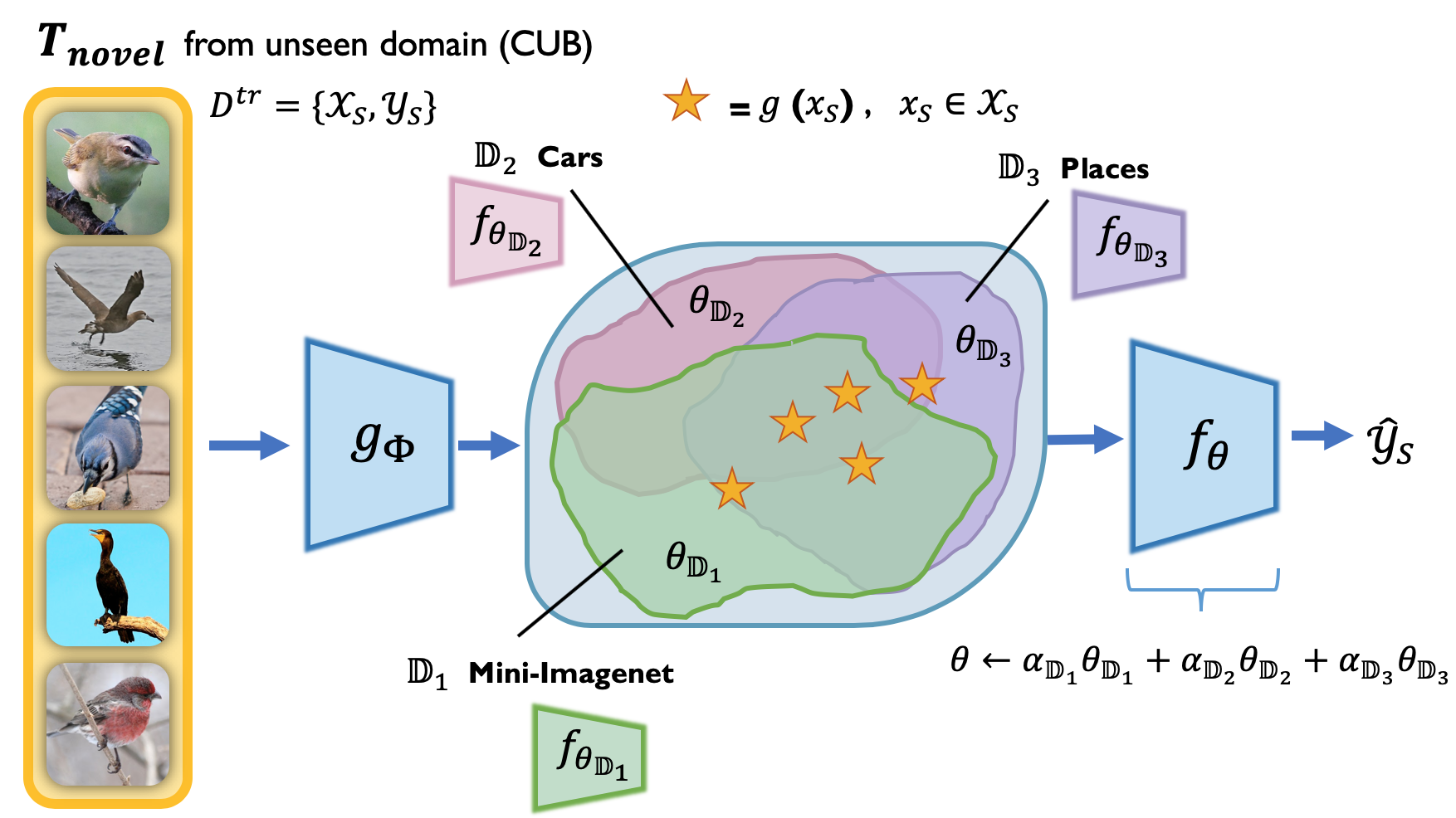
We define the problem as follows: Suppose we train a model on $M$ different seen domains $\mathbb{D}_{1}^{seen},\mathbb{D}_{2}^{seen},\dots,\mathbb{D}_{M}^{seen}$ in the meta-training stage, where each domain has an associated task distribution $p(T_{\mathbb{D}_{k}^{seen}}),k=1,...,M$ . Let $\mathbb{D}^{unseen}$ be an unseen domain with task distribution $p(T_{\mathbb{D}^{unseen}})$ . Our goal is to learn a model that can generalize to novel tasks $T_{novel}\sim p(T_{\mathbb{D}^{unseen}})$ during the meta-testing stage using the meta-learned prior knowledge from each of the $M$ seen domains. Figure 1 illustrates this problem setting.

4 Combining Domain-Specific Meta-Learners (CosML)

Our goal is to improve the cross-domain generalization ability of the model for few-shot classification on unseen domains. In order to achieve this goal, we propose to exploit the meta-parameters of all the different seen domains as a way to enable the few-shot classification model to generalize to novel target tasks from some unseen domain. In particular, our proposed solution takes a weighted combination of the domain-specific meta-parameters from each of the different seen domains to initialize a model that is then optimized for a novel target task from an unseen domain by performing a few steps of gradient descent.

Our deep neural network model consists of two subnetworks: a feature extractor $g_{\Phi}$ that extracts task-invariant features (see section 4.1) and a task subnetwork $f_{\theta}$ (see section 4.2) that extracts task-specific features and performs few-shot classification. CosML consists of three stages: pre-training, meta-training, and meta-testing. We explain each stage in detail in the following sections.

4.1 Pre-training

We apply a non-episodic approach to first pre-train a neural network to perform image classification, similar to the approach of chen2019closerlook (1). In our experiments, the non-episodic training set consists of the Mini-ImageNet dataset. After pre-training, we remove the final classification layer as well as the last two hidden layers of the network. This resulting network is the feature extractor $g_{\Phi}$ , which is then fixed to be used for subsequent stages. Our objective is to learn a non-task-specific representation for examples, in order to extract meaningful feature representations from the examples in a novel target task from some unseen domain $\mathbb{D}^{unseen}$ during meta-testing. Furthermore, we use the feature space determined by $g_{\Phi}$ to compare the similarity between novel tasks from an unseen domain and training tasks from the seen domains, which we will discuss in section 4.2.1.

4.2 Meta-training

The aim of meta-training is to train a set of domain-specific meta-learners that learn the meta-parameters, which are combined using similarity-based weights to initialize a task subnetwork $f_{\theta}$ for novel tasks from an unseen domain during meta-testing. The weights are determined by the similarity between the novel task and the computed domain and task prototypes belonging to each of the seen domains. The high-level meta-training procedure is shown in Algorithm 1.

Algorithm 1 CosML meta-training

1:Require: Pure task distributions

p(T_{\mathbb{D}_{1}}^{p}),\dots,p(T_{\mathbb{D}_{M}}^{p})

and mixed task distribution

p(T^{m})

2:Require: Hyper-parameters

\gamma,\beta

, pre-trained feature extractor

g_{\Phi}

3:Output:

M

meta-parameters

\theta_{\mathbb{D}_{k}}

and prototypes

P_{\mathbb{D}_{k}}=\{Z_{T\mathbb{D}_{k}},Z_{\mathbb{D}_{k}}\}

for

k=1,\dots,M

4:Randomly initialize

\theta_{\mathbb{D}_{1}},\dots,\theta_{\mathbb{D}_{M}}

5:while not done do

6: for each seen domain

\mathbb{D}_{k},k=1,\dots,M

\triangleright

Set 1: pure tasks

\triangleleft

7: Sample a batch of pure tasks

T_{j}^{p}\sim p(T^{p}_{\mathbb{D}_{k}})

8: for each task

T_{j}^{p}=(D_{T_{j}^{p}}^{tr},D_{T_{j}^{p}}^{val})

9: Compute new task prototype

z_{T_{j}}

using equation 1 and append it to

Z_{T\mathbb{D}_{k}}

10: Update

Z_{\mathbb{D}_{k}}

using equation 2

11: Compute adapted parameters with gradient descent using K examples per class:

\theta^{\prime}_{T_{j}^{p}}=\theta_{\mathbb{D}_{k}}-\gamma\nabla_{\theta_{\mathbb{D}_{k}}}\mathcal{L}_{T_{j}^{p}}(f_{\theta_{\mathbb{D}_{k}}}(g_{\Phi}(x));D_{T_{j}^{p}}^{tr})

12: end for

13: Update

\theta_{\mathbb{D}_{k}}\leftarrow\theta_{\mathbb{D}_{k}}-\beta\nabla_{\theta_{\mathbb{D}_{k}}}\sum_{T_{j}^{p}\sim p(T_{\mathbb{D}_{k}}^{p})}\mathcal{L}_{T_{j}^{p}}(f_{\theta^{\prime}_{T_{j}^{p}}}(g_{\Phi}(x));D_{T_{j}^{p}}^{val})

14: end for

15: Sample a batch of mixed tasks

T_{j}^{m}\sim p(T^{m})

\triangleright

Set 2: mixed tasks

\triangleleft

16: for each task

T_{j}^{m}=(D_{T_{j}^{m}}^{tr},D_{T_{j}^{m}}^{val})

17: Compute

\alpha_{\mathbb{D}_{k}{T_{j}^{m}}}

for

k=1,\dots,M

using equations 5 and 6

18: Compute

\theta=\alpha_{\mathbb{D}_{1}{T_{j}^{m}}}\theta_{\mathbb{D}_{1}}+\dots+\alpha_{\mathbb{D}_{M}{T_{j}^{m}}}\theta_{\mathbb{D}_{M}}

19: Compute adapted parameters with gradient descent using K examples per class:

\theta^{\prime}_{T_{j}^{m}}=\theta-\gamma\nabla_{\theta}\mathcal{L}_{T_{j}^{m}}(f_{\theta}(g_{\Phi}(x));D_{T_{j}^{m}}^{tr})

20: end for

21: Update each

\{\theta_{\mathbb{D}_{k}}|k=1,\dots,M\}

using equation 7

22:end while

4.2.1 Prototypes

Similar to and following the notations from snell2017protonet (21), we use task prototypes to represent training tasks used during meta-training in the feature space. Furthermore, we use domain prototypes to represent different domains in the feature space.

Let us first denote $S_{T\mathbb{D}_{k}}=\{T_{i}\;|\;T_{i}=\{D_{T_{i}}^{tr},D_{T_{i}}^{val}\},i=1,2,...\}$ as a set of training tasks from domain $\mathbb{D}_{k}$ used during meta-training; $S_{T\mathbb{D}_{k}}$ grows with the number of training iterations. Let $S_{\mathbb{D}}=\{(x,y)\in D_{T_{i}}^{tr}\cup\;D_{T_{i}}^{val}\;|\;T_{i}\in S_{T\mathbb{D}_{k}}\}$ be the set of all the training task examples belonging to domain $\mathbb{D}_{k}$ . Finally, let $P_{\mathbb{D}_{k}}=\{Z_{T\mathbb{D}_{k}},Z_{\mathbb{D}_{k}}\}$ denote the set of prototypes for domain $\mathbb{D}_{k}$ , which includes a growing set of task prototypes $Z_{T\mathbb{D}_{k}}$ and one domain prototype $Z_{\mathbb{D}_{k}}$ that is updated during meta-training. We formally define a task prototype $z_{T}\in Z_{T\mathbb{D}}$ as the average feature vector of all of the training (support) and validation (query) examples in a given training task $T$ that belongs to a specific domain $\mathbb{D}^{seen}$ :

z_{T}=\frac{1}{|D_{T}^{tr}\cup D_{T}^{val}|}\sum_{x\;\in D_{T}^{tr}\cup D_{T}^{val}}g_{\Phi}(x)

(1)

We also formally define a domain prototype as the average feature vector of all the examples from the training and validation set of training tasks used during meta-training from a given domain $\mathbb{D}^{seen}$ :²²2We omit the superscript $seen$ from $\mathbb{D}^{seen}$ for clarity.

Z_{\mathbb{D}}=\frac{1}{|S_{\mathbb{D}}|}\sum_{x\;\in S_{\mathbb{D}}}g_{\Phi}(x)

(2)

Task and domain prototypes are adaptively computed during meta-training as new training tasks are sampled and used to train the model. The set of task prototypes grows with an increasing number of training tasks, while the number of domain prototypes remains constant, although the domain prototypes themselves change.

Similarity between tasks and prototypes

We define the distance between a task $T$ and a prototype as the average distance between the training examples in the task and the prototype in the feature space determined by $g_{\Phi}$ :

ds(T,z)=\frac{1}{|D_{T}^{tr}|}\sum_{x_{i}\;\in D_{T}^{tr}}d(g_{\Phi}(x_{i}),z)

(3)

where $z$ is a (task or domain) prototype and $D_{T}^{tr}$ is the training set of task $T$ . $T$ is a mixed task $T^{m}$ (see section 4.2.2) during the meta-training stage and a novel task $T_{novel}$ at meta-test time. Finally, $d(\cdot,\cdot)$ is a distance function such as the Euclidean distance, which we are using in our implementation.

To determine the distance between a task and a seen domain $\mathbb{D}_{k}^{seen}$ , we consider both the distance to the domain prototype and the distance to all task prototypes corresponding to $\mathbb{D}_{k}^{seen}$ ³³3We again omit the superscript $seen$ from $\mathbb{D}_{k}^{seen}$ for clarity. as follows:

dist(T,\mathbb{D}_{k})=\frac{1}{2}\times[ds(T,Z_{\mathbb{D}_{k}})+\frac{1}{N_{Tk}}\sum_{z_{T}\in Z_{T\mathbb{D}_{k}}}ds(T,z_{T})]

(4)

where $N_{Tk}$ is the total number of training tasks used so far in $\mathbb{D}_{k}^{seen}$ . We compute $dist(T,\mathbb{D}_{k})$ for all the seen domains, $k=1,...,M$ .

The domain weight $\alpha_{\mathbb{D}_{k}}$ assigned to a seen domain $\mathbb{D}_{k}^{seen}$ is inversely proportional to its distance; the closer the task is to a domain in the feature space, the larger the weight will be for that domain:

\alpha_{\mathbb{D}_{k}}=1/dist(T,\mathbb{D}_{k})

(5)

To combine the domain-specific meta-learners (task subnetworks) by taking a weighted average of their meta-parameters, we normalize the domain weights as follows:

\alpha_{\mathbb{D}_{k}}=\alpha_{\mathbb{D}_{k}}/\sum_{j=1}^{M}\alpha_{\mathbb{D}_{j}}

(6)

4.2.2 Pure tasks and mixed tasks

Following the common practice of meta-learning, we use pure tasks – tasks that consist of classes (and examples) from a single domain – to episodically train a set of model parameters that can be quickly adapted to different tasks from the same domain. In addition, we propose to use mixed tasks – tasks that consist of randomly selected classes from different domains – in order to simulate novel tasks from an unseen domain and to update and regularize the domain-specific meta-parameters so that they will be able to adapt better to unseen domains in the meta-test phase.

In each iteration of our episodic training, we consider two sets of tasks. The first set consists of a mini-batch of pure tasks $T^{p}$ , where each task includes a training set $D_{T^{p}}^{tr}$ and a corresponding validation set $D_{T^{p}}^{val}$ . We first use the set of pure tasks to learn domain-specific meta-parameters, using the same meta-training procedure as MAML. The second set consists of a mini-batch of mixed tasks $T^{m}$ , where each task also includes $D_{T^{m}}^{tr}$ and $D_{T^{m}}^{val}$ . We treat the set of mixed tasks as novel tasks from some unseen domain and initialize their task subnetwork $f_{\theta}$ using the weighted average of the domain-specific meta-parameters $\theta_{\mathbb{D}_{1}},\dots,\theta_{\mathbb{D}_{M}}$ as follows: $\theta=\alpha_{\mathbb{D}_{1}}\theta_{\mathbb{D}_{1}}+\dots+\alpha_{\mathbb{D}_{M}}\theta_{\mathbb{D}_{M}}$ .

Based on the performance of $f$ on the mixed tasks after a few gradient steps using $D_{T^{m}}^{tr}$ , each of the domain-specific meta-parameters $\theta_{\mathbb{D}_{k}}$ will be updated accordingly:

\theta_{\mathbb{D}_{k}}\leftarrow\theta_{\mathbb{D}_{k}}-\beta\nabla_{\theta_{\mathbb{D}_{k}}}\sum_{T_{j}^{m}\sim p(T^{m})}\alpha_{\mathbb{D}_{k}T_{j}^{m}}\mathcal{L}_{T_{j}^{m}}(f_{\theta^{\prime}_{T_{j}^{m}}}(g_{\Phi}(x));D_{T_{j}^{m}}^{val})

(7)

where $\beta$ is the same meta step size used by MAML. In the above update step, the loss is computed by evaluating the adapted model $f$ , using updated task-specific parameters $\theta^{\prime}_{T_{j}^{m}}$ , on the validation set of mixed task $T_{j}^{m}$ . The task-specific parameters $\theta^{\prime}_{T_{j}^{m}}$ are learned using the training set of task $T_{j}^{m}$ .

4.3 Meta-testing

At meta-test time, we employ the meta-parameters of the domain-specific task subnetworks obtained from meta-training to learn a task subnetwork for novel tasks from an unseen domain $\mathbb{D}^{unseen}$ . To do so, we initialize a task subnetwork with the weighted average of the domain-specific meta-parameters, weighted by the similarity of these domains and a novel task $T_{novel}$ from $\mathbb{D}^{unseen}$ . This model is then optimized via a few steps of gradient descent using the training (support) set of $T_{novel}$ . The performance of the final model is evaluated on the test (query) set of $T_{novel}$ .

5 Experiments

5.1 Experimental setup

Dataset

We use the Mini-ImageNet ravi2017OptimizationAA (18), CUB welinder2010cub (30), Cars krause2013cars (11), Places zhou2017places (32), and Plantae vanhorn2018plantae (6) datasets to evaluate the cross-domain few-shot classification performance of CosML in comparison with existing few-shot learning methods. Additional details can be found in the Supplementary Material.

Table 1: Cross-domain few-shot classification accuracy. The dataset listed in each column represents the unseen domain while the remaining 4 datasets are seen domains used during meta-training. All the methods use the PT-miniImagenet pre-trained feature extractor. We include experimental results for MAML initialized with PT-miniImagenet and for MAML without any initialization, denoted by no-PT. All the methods use the Conv-4 backbone except for MatchingNet LFT* and RelationNet LFT*, which use the ResNet-10 he2016resnet (4) backbone. Results for MatchingNet LFT* and RelationNet LFT* are from tseng2020crossdomainfewshot (26).

5-way 1-shot
Method	CUB	Cars	Places	Plantae
MatchingNet LFT*	$43.29\pm 0.59\%$	$30.62\pm 0.48\%$	$52.51\pm 0.67\%$	$\textbf{35.12}\pm\textbf{0.54}\%$
RelationNet LFT*	$\textbf{48.38}\pm\textbf{0.63}\%$	$32.21\pm 0.51\%$	$50.74\pm 0.66\%$	$35.00\pm 0.52\%$
MatchingNet LFT tseng2020crossdomainfewshot (26)	$34.20\pm 0.53\%$	$30.15\pm 0.46\%$	$39.43\pm 0.60\%$	$29.50\pm 0.39\%$
RelationNet LFT tseng2020crossdomainfewshot (26)	$39.70\pm 0.58\%$	$32.59\pm 0.54\%$	$39.92\pm 0.59\%$	$33.11\pm 0.56\%$
ProtoNet snell2017protonet (21)	$36.54\pm 0.52\%$	$29.38\pm 0.42\%$	$40.12\pm 0.59\%$	$31.42\pm 0.49\%$
Proto-MAML triantafillou2019metadataset (25)	$36.05\pm 0.53\%$	$29.46\pm 0.44\%$	$38.71\pm 0.57\%$	$31.20\pm 0.49\%$
MAML finn2017maml (3) (no PT)	$35.06\pm 0.54\%$	$31.12\pm 0.54\%$	$36.14\pm 0.56\%$	$30.95\pm 0.49\%$
MAML finn2017maml (3)	$35.50\pm 0.53\%$	$26.76\pm 0.42\%$	$39.21\pm 0.60\%$	$31.35\pm 0.49\%$
Ours: CosML	$46.89\pm 0.59\%$	$\textbf{47.74}\pm\textbf{0.59}\%$	$\textbf{53.96}\pm\textbf{0.62}\%$	$30.93\pm 0.46\%$
5-way 5-shot
Method	CUB	Cars	Places	Plantae
MatchingNet LFT*	$61.41\pm 0.57\%$	$43.08\pm 0.55\%$	$64.99\pm 0.59\%$	$48.32\pm 0.57\%$
RelationNet LFT*	$64.99\pm 0.54\%$	$43.44\pm 0.59\%$	$67.35\pm 0.54\%$	$\textbf{50.39}\pm\textbf{0.52}\%$
MatchingNet LFT tseng2020crossdomainfewshot (26)	$49.09\pm 0.53\%$	$42.42\pm 0.53\%$	$54.15\pm 0.54\%$	$43.32\pm 0.53\%$
RelationNet LFT tseng2020crossdomainfewshot (26)	$55.53\pm 0.59\%$	$46.05\pm 0.55\%$	$53.17\pm 0.55\%$	$45.66\pm 0.56\%$
ProtoNet snell2017protonet (21)	$56.37\pm 0.53\%$	$43.83\pm 0.55\%$	$59.91\pm 0.56\%$	$\textbf{50.39}\pm\textbf{0.59}\%$
Proto-MAML snell2017protonet (21)	$57.21\pm 0.54\%$	$45.06\pm 0.56\%$	$58.38\pm 0.57\%$	$47.45\pm 0.55\%$
MAML finn2017maml (3) (no PT)	$53.20\pm 0.54\%$	$43.71\pm 0.56\%$	$53.91\pm 0.57\%$	$44.70\pm 0.53\%$
MAML finn2017maml (3)	$52.66\pm 0.52\%$	$43.43\pm 0.53\%$	$56.61\pm 0.58\%$	$42.72\pm 0.55\%$
Ours: CosML	$\textbf{66.15}\pm\textbf{0.63}\%$	$\textbf{60.17}\pm\textbf{0.63}\%$	${\color[rgb]{0,0,0}\textbf{88.08}\pm\textbf{0.46{}}}\%$	$42.96\pm 0.57\%$

Implementation details

We use the 4-module convolutional network (Conv-4) architecture that is commonly used in few-shot classification vinyals2016matchingnet (28, 3, 21). In our implementation of CosML, the feature extractor $g_{\Phi}$ consists of the first two modules, which are fixed, and the task subnetwork $f_{\theta}$ consists of the last two modules and a linear classification layer. Additional implementation details can be found in the Supplementary Material.

Pre-trained feature extractor

We denote the Conv-4 network that is pre-trained on the Mini-ImageNet dataset as PT-miniImagenet.

Baseline methods

The selected baseline methods include both within-domain and cross-domain metric- and optimization-based meta-learning methods: MatchingNet and RelationNet with learning-to-learned feature-wise transformation (LFT)⁴⁴4Implementation from https://github.com/hytseng0509/CrossDomainFewShot. tseng2020crossdomainfewshot (26), ProtoNet⁵⁵5Implementation from https://github.com/wyharveychen/CloserLookFewShot. snell2017protonet (21), MAML⁵ finn2017maml (3), and Proto-MAML⁶⁶6Implementation from https://github.com/google-research/meta-dataset. triantafillou2019metadataset (25). We initialize each baseline method as well as CosML with PT-miniImagenet. The entire pre-trained Conv-4 network is fine-tuned in the baseline methods, whereas we only use the first two modules of the pre-trained network as the feature extractor for our method and keep them fixed.

We follow the same leave-one-out experimental setup as tseng2020crossdomainfewshot (26). This means that only 4 out of the 5 datasets are used as seen domains during meta-training; the held out domain becomes the unseen domain. We do not tune any of the hyper-parameters for our method. For the baseline methods, we use the hyper-parameters that are provided in their original implementations. More experimental details can be found in the Supplementary Material.

Table 2: Ablation studies. The accuracies shown are for leave-one-out 5-way 5-shot cross-domain few-shot classification. CosML₁ uses uniform weights instead of similarity-based weights. CosML₂ is meta-trained without mixed tasks. CosML₃ uses a deeper feature extractor

g_{\Phi}

;

g_{\Phi}

contains 3 conv modules and

f_{\theta}

consists of 1 conv module and a classification layer. The PT-miniImagenet pre-trained feature extractor is used.

Method	CUB	Cars	Places	Plantae
CosML₁ (uniform $\alpha_{k}$ )	$86.46\pm 0.47\%$	$57.71\pm 0.60\%$	$72.36\pm 0.58\%$	$44.37\pm 0.55\%$
CosML₂ (no $T^{m}$ )	$35.26\pm 0.43\%$	$32.24\pm 0.41\%$	$31.95\pm 0.42\%$	$26.27\pm 0.35\%$
CosML₃ (deeper $g_{\Phi}$ )	$52.21\pm 0.59\%$	$41.21\pm 0.50\%$	$52.10\pm 0.61\%$	$26.51\pm 0.36\%$
Complete CosML	$66.15\pm 0.63\%$	$60.17\pm 0.63\%$	${\color[rgb]{0,0,0}88.08\pm 0.46}\%$	$42.96\pm 0.57\%$

5.2 Experimental results

Main results

Table 1 presents the accuracy of CosML and all the baseline methods for 5-way 1-shot and for 5-way 5-shot classification. All of the reported results represent the mean accuracy with a $95\%$ confidence interval of 1000 randomly sampled novel tasks from the selected unseen domain. We observe that CosML consistently outperforms all baseline methods for all unseen domains except for Plantae. We hypothesize the lack of performance improvement for CosML on the unseen domain Plantae is due to a large domain difference between the Plantae dataset and the other datasets. Metric-based baselines – MatchingNet LFT*, RelationNet LFT*, and ProtoNet – perform the best on the unseen domain Plantae. This is consistent with the experimental results from chen2019closerlook (1, 25), where metric-based methods are shown to outperform optimization-based methods when the domain difference is large. The performance of CosML is consistent in both the 5-way 1-shot and 5-shot settings. Our experimental results demonstrate the effectiveness of leveraging domain-specific knowledge by combining meta-learners in the parameter space.

Ablation studies

The results of our ablation studies are reported in Table 2. The performance decreases significantly without the use of mixed-tasks during meta-training. On the CUB and Plantae datasets, we observe better performance when using uniform weights instead of similarity-based weights to combine the domain-specific meta-learners. While this confirms the effectiveness of combining meta-learners, this also suggests that better similarity-based weighting schemes should be investigated in future research. Finally, we observe that increasing the depth of $g_{\Phi}$ by 1 conv module and decreasing the depth of $f_{\theta}$ by 1 conv module for CosML hurts the cross-domain performance substantially. This observation aligns with the experimental findings from yosinki2014how (31). Features that are more specific to the Mini-ImageNet (pre-training) dataset are transferred when we increase the depth of our pre-trained and fixed feature extractor $g_{\Phi}$ , which hurts the performance when we train the remaining layers of the network on a different dataset.

6 Conclusion

In this paper, we proposed a novel method for few-shot classification in the cross-domain setting, called Combining Domain-Specific Meta-Learners (CosML), that leverages the meta-learned knowledge from each of the seen training domains. More specifically, CosML combines the meta-learners by taking a weighted average of the domain-specific meta-parameters, which is used to initialize a new task subnetwork to quickly adapt to a novel task from an unseen domain. We show strong empirical results for CosML in comparison to the state-of-the-art within-domain and cross-domain few-shot learning methods. This shows the effectiveness of leveraging domain-specific knowledge by combining meta-learners in the parameter space.

To the best of our knowledge, CosML is the first meta-learning method that combines model parameters to support quick adaptation to tasks from an unseen domain. Not only is our method simple, it is also effective in a variety of settings. For future work, we believe it is important to investigate how to best divide the neural network into the feature extractor subnetwork and task subnetwork, i.e., how many fixed layers to use for the feature extractor and how many layers to use and train for the task subnetwork. Also, as CosML does not know the confidence of its cross-domain predictions, a method needs to be developed to assess the similarities of the novel tasks from an unseen domain to the seen domain(s) in order to compute confidences, which we leave for future research.

Acknowledgement

We would like to thank Shao-Hua Sun, Hossein Sharifi-Noghabi, Xiang Xu, Jialin Lu, and Yudong Luo for the discussions and support. We would also like to thank Compute Canada for providing the computational resources. This research was supported by the Natural Sciences and Engineering Research Council (NSERC) Discovery Grant "Data mining in heterogeneous information networks with attributes" (to Martin Ester).

References

(1) Wei-Yu Chen, Yen-Cheng Liu, Zsolt Kira, Yu-Chiang Frank Wang and Jia-Bin Huang “A Closer Look at Few-shot Classification” In International Conference on Learning Representations, 2019
(2) Jia Deng, Wei Dong, Richard Socher, Li-Jia Li, Kai Li and Li Fei-Fei “ImageNet: A large-scale hierarchical image database” In IEEE Conference on Computer Vision and Pattern Recognition, 2009
(3) Chelsea Finn, Pieter Abbeel and Sergey Levine “Model-Agnostic Meta-Learning for Fast Adaptation of Deep Networks” In International Conference on Machine Learning, 2017
(4) Kaiming He, Xiangyu Zhang, Shaoqing Ren and Jian Sun “Deep Residual Learning for Image Recognition” In IEEE Conference on Computer Vision and Pattern Recognition, 2016
(5) Nathan Hilliard, Lawrence Phillips, Scott Howland, Artem Yankov, Courtney D Corley and Nathan O Hodas “Few-shot learning with metric-agnostic conditional embeddings” In arXiv preprint arXiv:1802.04376, 2018
(6) Grant Van Horn, Oisin Mac Aodha, Yang Song, Chen Sun Yin Cui, Alex Shepard, Hartwig Adam, Pietro Perona and Serge Belongie “The inaturalist species classification and detection dataset” In IEEE Conference on Computer Vision and Pattern Recognition, 2018
(7) Sergey Ioffe and Christian Szegedy “Batch Normalization: Accelerating Deep Network Training by Reducing Internal Covariate Shift” In arXiv preprint arXiv:1502.03167, 2015
(8) Pavel Izmailov, Dmitrii Podoprikhin, Timur Garipov, Dmitry Vetrov and Andrew Gordon Wilson “Averaging Weights Leads to Wider Optima and Better Generalization” In arXiv preprint arXiv:1803.05407, 2018
(9) Diederik P Kingma and Jimmy Ba “Adam: A method for stochastic optimization” In arXiv preprint arXiv:1412.6980, 2014
(10) Gregory Koch “Siamese neural networks for one-shot image recognition”, 2015
(11) Jonathan Krause, Michael Stark, Jia Deng and Li Fei-Fei “3D Object Representations for Fine-Grained Categorization” In IEEE International Conference on Computer Vision Workshops, 2013
(12) Brenden M Lake, Ruslan Salakhutdinov and Joshua B Tenenbaum “Human-level concept learning through probabilistic program induction” In Science 350.6266 American Association for the Advancement of Science, 2015, pp. 1332–1338 DOI: 10.1126/science.aab3050
(13) Brenden M. Lake, Ruslan Salakhutdinov, Jason Gross and Joshua B. Tenenbaum “One shot learning of simple visual concepts” In CogSci, 2011
(14) Erik G Miller, Nicholas E Matsakis and Paul A Viola “Learning from one example through shared densities on transforms” In IEEE Conference on Computer Vision and Pattern Recognition, 2000
(15) Tsendsuren Munkhdalai and Hong Yu “Meta Networks” In International Conference on Machine Learning, 2017
(16) Alex Nichol and John Schulman “Reptile: a Scalable Metalearning Algorithm” In arXiv preprint arXiv:1803.02999, 2018
(17) Minseop Park, Jungtaek Kim, Saehoon Kim, Yanbin Liu and Seungjin Choi “MxML: Mixture of Meta-Learners for Few-Shot Classification” In arXiv preprint arXiv:1904.05658, 2019
(18) Sachin Ravi and Hugo Larochelle “Optimization as a Model for Few-Shot Learning” In International Conference on Learning Representations, 2017
(19) Andrei A. Rusu, Dushyant Rao, Jakub Sygnowski, Oriol Vinyals, Razvan Pascanu, Simon Osindero and Raia Hadsell “Meta-Learning with Latent Embedding Optimization” In International Conference on Learning Representations, 2019
(20) Adam Santoro, Sergey Bartunov, Matthew Botvinick, Daan Wierstra and Timothy Lillicrap “Meta-Learning with Memory-Augmented Neural Networks” In Proceedings of The 33rd International Conference on Machine Learning, 2016
(21) Jake Snell, Kevin Swersky and Richard Zemel “Prototypical Networks for Few-shot Learning” In Advances in Neural Information Processing Systems, 2017
(22) Flood Sung, Yongxin Yang, Li Zhang, Tao Xiang, Philip H.S. Torr and Timothy M. Hospedales “Learning to Compare: Relation Network for Few-Shot Learning” In IEEE Conference on Computer Vision and Pattern Recognition, 2018
(23) Sebastian Thrun and Lorien Pratt “Learning to learn” In Springer Science & Business Media, 2012
(24) Eleni Triantafillou, Richard Zemel and Raquel Urtasun “Few-shot learning through an information retrieval lens” In Advances in Neural Information Processing Systems, 2017, pp. 2255–2265
(25) Eleni Triantafillou, Tyler Zhu, Vincent Dumoulin, Pascal Lamblin, Utku Evci, Kelvin Xu, Ross Goroshin, Carles Gelada, Kevin Swersky, Pierre-Antoine Manzagol and Hugo Larochelle “Meta-Dataset: A Dataset of Datasets for Learning to Learn from Few Examples” In International Conference on Learning Representations, 2020
(26) Hung-Yu Tseng, Hsin-Ying Lee, Jia-Bin Huang and Ming-Hsuan Yang “Cross-Domain Few-Shot Classification via Learned Feature-Wise Transformation” In International Conference on Learning Representations, 2020
(27) Joaquin Vanschoren “Meta-Learning: A Survey” In arXiv preprint arXiv:1810.03548, 2018
(28) Oriol Vinyals, Charles Blundell, Timothy Lillicrap, koray and Daan Wierstra “Matching Networks for One Shot Learning” In Advances in Neural Information Processing Systems, 2016
(29) Risto Vuorio, Shao-Hua Sun, Hexiang Hu and Joseph J. Lim “Multimodal Model-Agnostic Meta-Learning via Task-Aware Modulation” In Neural Information Processing Systems, 2019
(30) Peter Welinder, Steve Branson, Takeshi Mita, Catherine Wah, Florian Schroff, Serge Belongie and Pietro Perona “Caltech-UCSD Birds 200”, 2010
(31) Jason Yosinki, Jeff Clune, Yoshua Bengio and Hod Lipton “How transferable are features in deep neural networks?” In Advances in Neural Information Processing Systems, 2014
(32) Bolei Zhou, Agata Lapedriza, Aditya Khosla, Aude Oliva and Antonio Torralba “Places: A 10 million Image Database for Scene Recognition” In IEEE Transactions on Pattern Analysis and Machine Intelligence IEEE, 2017

Appendix A Datasets

For our cross-domain few-shot classification experiments, we use the Mini-ImageNet, CUB (birds), Cars, Places, and Plantae datasets. We follow the data pre-processing procedure from ravi2017OptimizationAA (18) and hilliard2018cubsplits (5) for the Mini-ImageNet and CUB datasets respectively. We follow the data pre-processing procedure from tseng2020crossdomainfewshot (26) for the Cars, Places, and Plantae datasets. Table 1 shows a summary of each dataset, which includes the dataset source, the data splits used, as well as the number of classes in each of the train, validation, and test splits.

The Mini-ImageNet dataset contains images of a variety of ojects. The CUB, Cars, Places, and Plantae datasets are fine-grained datasets that contain images of different species of birds, cars, places, and plants respectively.

Table 3: Dataset details. This table shows the dataset source, origin of the dataset splits used in the experiments, as well as the number of classes in each of the train, validation, and test splits.

Dataset	Source	Split used	Train classes	Validation classes	Test classes
Mini-ImageNet	Deng et al. deng2009imagenet (2)	Ravi & Larochelle ravi2017OptimizationAA (18)	64	16	20
CUB (birds)	Welinder et al. welinder2010cub (30)	Hilliard et al. hilliard2018cubsplits (5)	100	50	50
Cars	Krause et al. krause2013cars (11)	Tseng et al. tseng2020crossdomainfewshot (26)	98	49	49
Places	Zhou et al. zhou2017places (32)	Tseng et al. tseng2020crossdomainfewshot (26)	183	91	91
Plantae	Van Horn et al. vanhorn2018plantae (6)	Tseng et al. tseng2020crossdomainfewshot (26)	100	50	50

Appendix B Additional experimental details

B.1 Implementation details

Network architecture

We use the 4-module convolutional network (Conv-4) architecture that is commonly used in few-shot classification vinyals2016matchingnet (28, 3, 21). Each of the four modules consists of a $3\times 3$ convolutional layer with 64 output channels, followed by a batch normalization layer ioffe2015batch (7), a ReLU activation function, and finally a $2\times 2$ max pooling layer. Outputs from the last module are 1600-dimensional feature vectors, which are inputs to the linear layer for $N$ -way classification. In our experiments, we use the same Conv-4 backbone for CosML and for all the baseline methods.

In our implementation of CosML, the feature extractor $g_{\Phi}$ consists of the first two modules and the task subnetwork $f_{\theta}$ consists of the last two modules and a linear classification layer. Note that the feature space determined by $g_{\Phi}$ is 28224-dimensional. All the images are resized to size $84\times 84$ .

We will make the code for the implementation of our proposed method, CosML, publicly available on GitHub.

B.2 Hyper-parameters

Optimizer

In all of our experiments, we use the Adam optimizer kingma2014adam (9) with default settings from PyTorch. The hyper-parameter values in the default setting are: the learning rate is 0.001, the betas coefficients are (0.9, 0.999), the eps term is 1e-8, weight_decay is 0, and the amsgrad flag is set to False.

Metric-based methods

We use the same hyper-parameters as Tseng et al. tseng2020crossdomainfewshot (26) for training the MatchingNet LFT and RelationNet LFT models on the Conv-4 backbone. We use the same hyper-parameters as Snell et al. snell2017protonet (21) for training the ProtoNet models. However, rather than using a higher number of way for training the ProtoNet models, we use the same number of way (i.e., 5-way) as the tasks we use to evaluate the model during meta-testing to ensure fairness and consistency with the other models. The validation (query) set contains 16 images.

Optimization-based methods

We use the same hyper-parameters for MAML, Proto-MAML, and CosML in both the 5-way 1-shot and 5-way 5-shot settings. All the models are trained using a slow outer-loop learning rate (meta-step size) of 0.001, a fast inner-loop learning rate (step size) of 0.01, 5 gradient steps, a meta-batch size of 4 tasks, and a validation (query) set of 16 images. For CosML, the mini-batch sizes that we use for pure tasks and for mixed tasks are $25\times M$ and $25$ , respectively, where $M$ is the number of seen domains. A mini-batch of pure tasks contains the same number of tasks from each domain.

B.3 Training configurations

Hardware

We train all of the models, except for Proto-MAML, on a single NVIDIA V100SXM2 GPU with 16G of memory. Due to insufficient GPU memory, we train all Proto-MAML models on a CPU node with 60G of memory.

Training

All the few-shot classification models are trained using a total of 40,000 training tasks.