Combining TMD factorization and collinear factorization
Abstract
We examine some of the complications involved when combining (matching) TMD factorization with collinear factorization to allow accurate predictions over the whole range of measured transverse momentum in a process like Drell-Yan. Then we propose some improved methods for combining the two types of factorization. (This talk is based on work reported in arXiv:1605.00671.)
I Introduction
This talk was based on Collins et al. (2016), and provides a summary of the results there. More detailed references to earlier literature can be found in that paper.
The issue addressed is the matching of transverse-momentum-dependent (TMD) and collinear factorization for processes like the Drell-Yan process, with both a hard scale and a separate measured transverse momentum . TMD factorization applies when , and its accuracy degrades as increases towards . It involves TMD parton densities (pdfs) , and in more general process also TMD fragmentation functions.
In contrast, collinear factorization applies at large (i.e., of order ), and it also applies to the cross section integrated over all (and hence for the integral over up to a maximum of order ). Collinear factorization involves “collinear pdfs” . Its accuracy degrades as decreases, and collinear factorization by itself provides unphysically singular cross sections as . But the nature of the degradation is constrained by the fact the collinear factorization also applies to the cross section integrated over .
To get full accuracy over all one may combine both methods suitably. Collins, Soper, and Sterman (CSS) Collins and Soper (1982); Collins et al. (1985) implemented this as a kind of simple matched asymptotic expansion. But it has become increasingly clear—e.g., Boglione et al. (2015a, b)—that improved matching methods are needed to get adequate performance in practice, especially at the relatively low used in many experiments on semi-inclusive deep-inelastic scattering (SIDIS). These are of particular relevance to this conference, since these experiments measure important transverse spin asymmetries analyzed with the aid of TMD factorization, as can be seen from other contributions at the conference.
We will summarize the issues and then our proposed improvements in the matching methods.
II Key approximations to get TMD and collinear factorization
The essential measure of the quality of the applicability of a matching method is an evaluation of its accuracy. This is determined by the accuracy of the approximations used in deriving factorization from the exact cross section. The approximations can be understood from an examination of the derivations, as in Collins (2011). A simple example is given by the Feynman-graphical structure of the basic parton-model form, Fig. 1, where the Drell-Yan pair is created by quark-antiquark annihilation, with the quark and antiquark arising from structures that are collinearly moving with respect to the incoming hadrons.
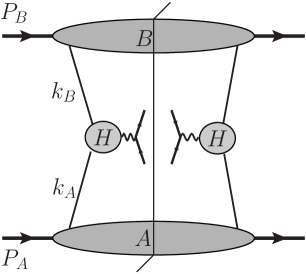
We use light-front coordinates, where the parton momenta are
| (1) |
The incoming hadrons and have large 3-momenta in the and directions, with no transverse momentum.
II.1 TMD factorization
To get the corresponding contribution to a TMD-factorized form, approximations are made: (a) In the hard-scattering subgraph, , the exact parton momenta and are replaced by on-shell values. (b) But in the kinematics, parton transverse momentum is retained, so that the virtual photon momentum is . Thus, after the approximations, the dependence on the small components and is confined to the subgraphs and , respectively, while the transverse momentum of the Drell-Yan pair arises from the quark transverse momenta.
We can then integrate over within and within , to obtain the natural contributions to the usually defined TMD pdfs. The approximations are valid because , etc. The approximations become bad when increases to roughly order .
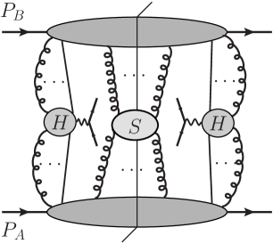
Other graphical structures giving leading power contributions, Fig. 2 are treated similarly, with the application of Ward identities and unitarity-style cancellations to get the TMD-factorized form.
II.2 Collinear factorization for large , and for integral over
Large is dominantly generated from hard scatterings where extra partons are emitted, exemplified in Fig. 3. The appropriate leading-power approximation for the hard scattering now neglects the transverse momenta of the incoming partons and , as well as their virtuality. Each collinear pdf is therefore defined with an integral over transverse momentum, and therefore depends kinematically only on the longitudinal momentum fraction of the parton.
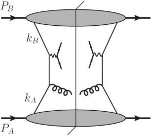
The collinear approximation involves neglecting small transverse momenta of the incoming partons in comparison with , as well as neglecting their virtualities. Therefore the approximation completely breaks down once is of order a typical transverse momentum for the partons entering the hard scattering. A symptom of the breakdown is the well-known strong singularity at of fixed-order calculations of the Drell-Yan cross section.
Next we turn to the cross section integrated over . Here one must include all the contributions at low . But now the collinear approximation remains valid, unlike the TMD case. In graphs like Fig. 1, the collinear approximation ignores the partonic in the hard scattering, which shifts the virtual photon’s transverse momentum to zero from its true value. But since this is just a shift, it leaves the integral over unchanged, to leading power in the large scale . Thus although collinear factorization is incorrect at low for the distribution in , it is nevertheless valid for the integral over .
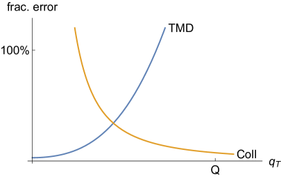
II.3 Error sizes
The qualitative behavior of the fractional errors in TMD and collinear factorization is shown in Fig. 4. TMD factorization is accurate at low up to relative errors suppressed by a power of , but it is totally inaccurate at of order . Collinear factorization for the distribution has the opposite behavior.
III CSS’s method to combine TMD and collinear factorization
CSS implemented the combination of TMD and collinear factorization by
| (2) |
where is the TMD factorized form
| (3) |
and is a collinear correction term
| (4) |
In , the convolution over the two TMD pdfs is rewritten as a Fourier transform over a transverse position variable .
The errors in and caused by the approximations in the derivations can be estimated as:
| (5) |
for when ,
| (6) |
for when . Here is some fixed positive number determined by QCD and the power-law errors in the approximations used in deriving factorization. To these errors are to be added truncation errors of perturbative calculations. Hence the error in Eq. (2) is estimated to be a uniform power of by
| (7) |
over the range . As one increases from order , the deviation of from the cross section increases. But a collinear approximation can be applied to this deviation. As increases the deviation becomes larger, while its collinear approximation becomes better, in proportion.
It is very important that the stated error estimate for TMD factorization applies only when , and can completely fail for higher . Similarly the stated error for collinear factorization applies only when , and can completely fail at lower .
IV What is problematic with the original formulation?
Boglione et al. (2015a, b) have found particular difficulties with implementing CSS’s method in SIDIS at moderately low energies. These are illustrated in Fig. 5, for SIDIS at at HERA. The solid line is the NLO calculation from collinear factorization. It shows the decrease of the cross section with hadron transverse that QCD predicts at the larger values of . But the NLO curve diverges as , where fixed-order calculations in collinear factorization are totally inaccurate.

The dotted curve shows the term, i.e., the result of TMD factorization, with fits to data determining the non-perturbative part of the TMD functions and their evolution. At small enough , it should be a good approximation by itself for the cross section.
The asymptotic low part of the NLO collinear-factorization term is given by the dashed curve labeled “ASY”. This reproduces the NLO calculation at low , but deviates from it substantially as increases. The deviation becomes substantial at quite a large factor below , which shows that there is a substantial numerical degradation of the simplest error estimates that were given in Sec. III. The ASY term goes through zero at around and then becomes negative.
Since the basic low asymptote has a logarithm: , the negative values are expected, and are in a region where the asymptotic calculation is inapplicable. The bothersome issue is that the inapplicability happens at what appears to be a surprisingly low compared with . Similarly goes through zero; this is also expected. The principle of the CSS method is that there should be a region of intermediate or where neither TMD nor collinear factorization is completely degraded in accuracy, at least for high . In this case, the large part of the TMD factorization and the low part of collinear factorization should approximately match. But this does not happen in Fig. 5. Furthermore the zeros in and ASY happen at quite different .
The term is the difference between the fixed-order collinear calculation, in this case NLO, and its small- asymptotic ASY. CSS intended this to correct TMD factorization to collinear factorization at large or . It is calculated to be small when is small, as it should be. But it quickly becomes much larger than the presumably approximately correct NLO estimate for the cross section, which rather invalidates its use as a correction.
These plots suggest some ideas for improving the method.
Perhaps the most important practical problem is that the TMD term, , goes negative at large . This indicates that at large , is the difference between substantially larger terms, and therefore shows a strong magnification of the relative effects of truncation errors in the predicted perturbative parts of the cross section.
Associated with this is that the integral over is exactly zero. This is because in -space, the evolution equations show that the integrand is zero: .
From these properties arises a severe problem in getting the integral over of the formula in Eq. (2) to agree with the collinear factorization results
-
•
On the left-hand side, the integral is given by collinear factorization starting at LO, i.e., , up to a power-suppressed error. Fixed-order calculations of the hard scattering are appropriate.
-
•
On the right-hand side, the integral of is zero. So the integral of the right-hand side is the integral of plus the error term.
-
•
But is obtained from collinear factorization starting at NLO, i.e., .
If we used a fixed order of collinear factorization, there is a mismatch of orders of , and this results in complete mismatch of sizes even at the highest . Recall that the elementary derivation of the formula concerned the errors at intermediate and did not concern itself explicitly with the integral over .
As regards the integral over all , we deduce that either we need resummation of to handle the problem, or the error term is intrinsically very large, or both. The knowledge that nevertheless fixed-order calculations with collinear factorization are completely appropriate for the integrated cross section motivates part of our method for improving the method.
V Our new proposal
We modify in two ways, as exhibited in our formula for a modified term:
| (8) |
First, to avoid problems in , we provide the function with a smooth cutoff at small :
| (9) |
The integral of (8) over is now given by at of order . This is correctly predicted by fixed-order collinear factorization, and agrees with collinear factorization for the integrated cross section at leading order. Higher-order terms bring in the integral of our correspondingly modified term, with well-behaved collinear expansions. This prescription is close to that of Bozzi et al. (2006). Their prescription was formulated purely in terms of resummation calculations in massless QCD. Our solution applies to full TMD factorization. The function has the same functional form as before, and involves exactly the same TMD pdfs and evolution equations; the modification consists in changing the value used for the transverse position argument in the Fourier transform, from to . At low , larger values of than dominate, and then the cutoff at small is unimportant; thus the validity of TMD factorization in its target region of is unaffected.
The second change is to impose an explicit cutoff at large cutoff, by a factor
| (10) |
This keeps the modified term from being significantly nonzero at such large that TMD factorization is totally inapplicable.
Correspondingly, to implement a correct matching, we modify to
| (11) |
The second factor is the basic implementation of matching of TMD and collinear factorization. But we impose an extra cutoff factor, for example
| (12) |
The reason for the extra cutoffs on at large and on at small is found in the derivation of the errors in Sec. III. That error calculation is only valid when . Below that range, we should use only the TMD factorization term , i.e., should then be close to zero. Above that range, we should only use collinear factorization, so should then be close to zero.
VI Conclusions
We modified the formalism, so that
-
•
The error in is suppressed by a power of for all .
-
•
The integral over all is now properly behaved with respect to collinear factorization for the integrated cross section.
Further improvements are undoubtedly possible. We have tried to formulate some relevant issues. Generally, to do better, one needs to “look under hood”, to ask questions like:
-
•
What is the nature of the approximations giving factorization (TMD and collinear)?
-
•
How much do they fail, with proper account of non-perturbative properties?
These issues are important for subject of this conference, i.e., spin physics. This is because we often want to use TMD factorization at moderate , notably in the measurement of transverse-spin-dependent TMD pdfs and fragmentation functions.
One important question for SIDIS, is to determine the appropriate criteria for what is large and small transverse momentum relative to . Is the appropriate variable or ? I.e., is it transverse momentum of the virtual photon relative to the detected hadrons, or is it the transverse-momentum of the detected final-state hadron relative to the and target? These two variables differ by a factor of the fragmentation variable . One can also ask whether that was even the right question.
It would also be useful to have the -term for SIDIS at NNLO, i.e., . This could be obtained from the results for collinear factorization for SIDIS at the same order, as reported by Daleo et al. Daleo et al. (2005), but we are not aware that this has been done yet.
Acknowledgements.
This work was supported by DOE contracts No. DE-AC05-06OR23177 (A.P., T.R., N.S., B.W.), under which Jefferson Science Associates, LLC operates Jefferson Lab, No. DE-FG02-07ER41460 (L.G.), and No. DE-SC0013699 (J.C.), and by the National Science Foundation under Contract No. PHY-1623454 (A.P.).References
- Collins et al. (2016) J. Collins, L. Gamberg, A. Prokudin, T. C. Rogers, N. Sato, and B. Wang, “Relating transverse momentum dependent and collinear factorization theorems in a generalized formalism,” Phys. Rev. D94, 034014 (2016), arXiv:1605.00671 [hep-ph] .
- Collins and Soper (1982) John C. Collins and Davison E. Soper, “Back-to-back jets: Fourier transform from to ,” Nucl. Phys. B197, 446–476 (1982).
- Collins et al. (1985) J. C. Collins, D. E. Soper, and G. Sterman, “Transverse momentum distribution in Drell-Yan pair and and boson production,” Nucl. Phys. B250, 199–224 (1985).
- Boglione et al. (2015a) M. Boglione, J. O. Gonzalez Hernandez, S. Melis, and A. Prokudin, “A study on the interplay between perturbative QCD and CSS/TMD formalism in SIDIS processes,” JHEP 02, 095 (2015a), arXiv:1412.1383 [hep-ph] .
- Boglione et al. (2015b) Mariaelena Boglione, J. Osvaldo Gonzalez Hernandez, Stefano Melis, and Alexei Prokudin, “Phenomenological implementations of TMD evolution,” Proceedings, QCD Evolution Workshop (QCD 2014): Santa Fe, USA, May 12-16, 2014, Int. J. Mod. Phys. Conf. Ser. 37, 1560030 (2015b), arXiv:1412.6927 [hep-ph] .
- Collins (2011) J. C. Collins, Foundations of Perturbative QCD (Cambridge University Press, Cambridge, 2011).
- Bozzi et al. (2006) Giuseppe Bozzi, Stefano Catani, Daniel de Florian, and Massimiliano Grazzini, “Transverse-momentum resummation and the spectrum of the Higgs boson at the LHC,” Nucl. Phys. B737, 73–120 (2006), arXiv:hep-ph/0508068 [hep-ph] .
- Daleo et al. (2005) A. Daleo, D. de Florian, and R. Sassot, “ QCD corrections to the electroproduction of hadrons with high transverse momentum,” Phys. Rev. D71, 034013 (2005), arXiv:hep-ph/0411212 [hep-ph] .