ComFairGNN: Community Fair Graph Neural Network
Abstract.
Graph Neural Networks (GNNs) have become the leading approach for addressing graph analytical problems in various real-world scenarios. However, GNNs may produce biased predictions against certain demographic subgroups due to node attributes and neighbors surrounding a node. Most current research on GNN fairness focuses predominantly on debiasing GNNs using oversimplified fairness evaluation metrics, which can give a misleading impression of fairness. Understanding the potential evaluation paradoxes due to the complicated nature of the graph structure is crucial for developing effective GNN debiasing mechanisms. In this paper, we examine the effectiveness of current GNN debiasing methods in terms of unfairness evaluation. Specifically, we introduce a community-level strategy to measure bias in GNNs and evaluate debiasing methods at this level. Further, We introduce ComFairGNN, a novel framework designed to mitigate community-level bias in GNNs. Our approach employs a learnable coreset-based debiasing function that addresses bias arising from diverse local neighborhood distributions during GNNs neighborhood aggregation. Comprehensive evaluations on three benchmark datasets demonstrate our model’s effectiveness in both accuracy and fairness metrics.
1. Introduction
In today’s interconnected world, graph learning supports various real-world applications, such as social networks, recommender systems , and knowledge graphs (Bourigault et al., 2014; Nickel et al., 2015). Graph Neural Networks (GNNs) are powerful for graph representation learning and are used in tasks like node classification and link prediction by aggregating neighboring node information. However, GNNs often overlook fairness, leading to biased decisions due to structural bias and attribute bias like gender, race, and political ideology. These bias can cause ethical dilemmas in critical contexts, such as job candidate evaluations, where a candidate might be favored due to shared ethnic background or mutual acquaintances.
To tackle the outlined issue, multiple methods were suggested to evaluate and mitigate the fairness of node representation learning on graphs. Most of these methods aim to learn node representations that can yield statistically fair predictions across subgroups defined based on sensitive attributes (Lambrecht and Tucker, 2019; Kamishima and Akaho, 2017; Saxena et al., 2022). Choosing the right metric to evaluate bias in graphs inherently depends on the specific task at hand. The existing methods employed graph-level metrics originally designed for other purposes to address fairness concerns. The primary difficulty in addressing fairness within graphs arises from the frequent correlation between the graph’s topology and the sensitive attribute we aim to disregard. However, due to the complicated nature of graph structures, conducting graph-level fairness evaluations and comparisons of different methods is not as straightforward as commonly reported in the existing methods.
Recently works (Xu et al., 2018; Kusner et al., 2017; Gölz et al., 2019; von Kügelgen et al., 2021) point out that the reported scores in prior works might not reflect the true performance in the real-world application because of various evaluation issues and the nature of the dataset. For example, Simpson’s paradox (Blyth, 1972), highlights the context of the graduate admissions bias at UC Berkeley in 1973. Historically, it was believed that 44% of the 8,442 male applicants were admitted, compared to 35% of the 4,342 female applicants, indicating a gender bias. However, a closer look reveals that four out of the six departments had a higher acceptance rate for women, while two departments had a higher acceptance rate for men. A recent example of Simpson’s paradox during the COVID-19 era illustrates its implications in health policy. In 2020, initial data showed a higher COVID-19 case fatality rate in Italy than in China. However, this analysis was confounded by age distribution differences. When analyzed by age groups, the case fatality rate was actually higher in China than in Italy within each age group (von Kügelgen et al., 2021). The aforementioned works are not focused on fairness for machine learning on graphs.
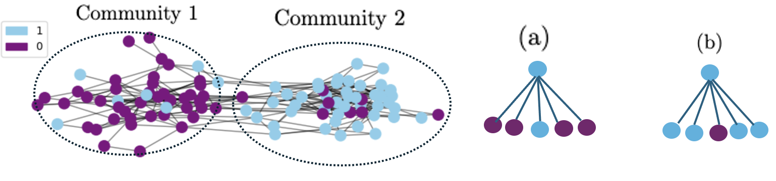
The majority of real-world graphs are polarized into communities due to some sensitive features such as age, gender, race, ideology, and socio-economic status, as shown in figure 1. A community is a group of nodes that are highly interconnected within the group and have fewer connections to nodes outside the group. For instance, research indicates that the dynamics of interaction among communities within United States Twitter networks are significantly shaped by their political allegiances (Guerra et al., 2013). Within the country, the flow of communication between communities in the Northeast and West Coast is largely driven by Democratic supporters, contrasting with the influence of Republican supporters. Conversely, in Texas, Florida, and Iowa, Republican supporters tend to dominate the network flow. This suggests a geographical alternation bubble in the dominance of network flows between Democrat and Republican communities. Consider a scenario where social media users are categorized into those who like basketball and those who like football. The demographics of those subgroups may vary across different regions despite the existence of some individuals who participate in both sports.
In this paper, we investigate the important problem of community fairness in graph neural networks in the context of node classification. On the one hand, simply employing node attribute and their structure debiasing function may result in misleading fairness evaluation and loss of information (Wu et al., 2019). Communities are a manifestation of the local neighborhood structures, which are fundamentally different from a sensitive node attribute (Rahman et al., 2019). Particularly, in GNNs, each node learns by aggregation of information from the neighboring nodes, thus identical label nodes with varying neighborhood distribution as illustrated in figure 1, giving rise to structural bias in the learning process. Moreover, the bias may be further amplified by multi-layered recursive neighborhood aggregation in GNNs. Although current debiasing methods primarily address attribute-based node fairness, they fail to tackle the fundamental bias inherent in GNN neighborhood aggregation. Consequently, these approaches are unable to effectively mitigate local community-level biases arising from disparate neighborhood structures.
To address community fairness, we introduce the concept of local structural fairness at the community level for all nodes in the graph. This approach recognizes that the broader structural bias affecting nodes within a community emerges from the GNN’s aggregation process, which is influenced by the diverse distribution of local neighborhoods. We present ComFairGNN, a novel community-fair Graph Neural Network compatible with any neighborhood aggregation-based GNN architecture. Specifically, the coreset-based debiasing function targets the neighborhood aggregation of GNN operation, aiming to bring identical label nodes closer in the embedding space. This approach mitigates structural disparities across communities, leading to fairer representations for nodes with identical labels.
In summary, our paper makes three key contributions: (1) We measure the problem of fairness and potential evaluation paradoxes at the community level using different fairness evaluation metrics in GNNs. (2) We propose a novel community fairness for GNNs named ComFairGNN that can balance the structural bias for identical label nodes in different communities. ComFairGNN works with any neighborhood aggregation-based GNNs. (3) Comprehensive empirical evaluations validate our method’s effectiveness in enhancing both fairness and accuracy.
2. PRELIMINARIES
In this section, we introduce the structural-based clustering setting to assess our research question: to what extent are the existing graph fairness evaluation metrics prevalent in fair decisions at the community level and prevent the corresponding types of fairness paradoxes?
Let’s first introduce the notations. A graph consists of nodes and edges . The node-wise feature matrix has dimensions for raw node features, with each row representing the feature vector for the -th node. The binary adjacency matrix is , and the learned node representations are captured in , where is the latent dimension size and is the representation for the -th node. The sensitive attribute classifies nodes into demographic groups, with edges being intragroup if and intergroup otherwise. The function returns the set of neighbors for a node , providing a structural node embedding. Clusters based on this embedding are denoted as , with for nodes in the -th cluster and as the cluster count. Each represents a community and measures the statistical notion of fairness across different communities in the graph.
2.1. Graph Neural Network
Graph Neural Networks (GNNs) utilize a layered architecture for neighborhood aggregation, where nodes progressively integrate information from their immediate neighbors across multiple iterations. For the -th layer, the representation of a node , denoted as , is formulated as follows:
| (1) |
where is the dimension of node representations in the -th layer, denotes an aggregation function such as mean-pooling (Kipf and Welling, 2016) or self-attention (Veličković et al., 2017), is an activation function, denotes the set of neighbors of , and denotes the learnable parameters in layer . The initial layer (layer 0) utilizes the raw input features as node representations, expressed mathematically as , where denotes the input attribute vector for node .
2.2. Node Clustering on Structural Embedding
By integrating node2vec (Grover and Leskovec, 2016) embeddings with -means clustering (MacQueen et al., 1967), we can effectively partition the graph into communities based on the structural similarities captured by the embeddings.
Graph embedding using node2vec is a mapping that assigns each node in a graph to a vector in a -dimensional space, denoted as , where is a hyperparameter representing the number of dimensions in the vector space. For each node in a graph , multiple random walks are performed, as specified by the hyperparameter walk_num. This process generates a list of sequences, each comprising node IDs from individual random walks. A single random walk follows the standard approach in unweighted graphs, where at each step, the next node is selected uniformly at random from the current node’s neighbors. The hyperparameters walk_num and walk_len control the number of walks and the length of each walk, respectively. Next, node2vec uses the generated sequences to train a neural network and learn embedding vectors. Let us define a network neighborhood as the set of nodes preceding and succeeding node in the generated walk sequences. The objective function is defined as:
| (2) |
is the conditional probability represented as softmax.
Once the node embeddings are learned using node2vec, the next step involves clustering these embeddings to identify groups of similar nodes. Our primary focus for clustering is on -means clustering, selected for its efficient linear runtime. -means aims to minimize the total sum of squared errors, also known as inertia or within-cluster sum of squares (Shiao et al., 2023). This objective can be formally expressed as:
| (3) |
2.3. Group Fairness Metrics on Graphs
We specifically target group fairness scenarios where both the node label and the sensitive attribute are binary. Group fairness is the most prevalent and extensively studied form of fairness. In the context of group fairness, we consider a model or algorithm to be fair when its outputs exhibit no bias against any demographic group of sensitive attributes. In this work, we primarily focus on assessing the evaluation of existing graph fairness methods utilizing the two widely used metrics of group fairness, i.e., demographic parity (Dwork et al., 2012) and equal opportunity (Hardt et al., 2016).
Let denote the prediction output of the classifier . and represent the ground truth and the sensitive attribute, respectively.
Demographic Parity: Demographic parity, also referred to as statistical parity, necessitates that the prediction is independent of the sensitive attribute , symbolized as . Formally, demographic parity aims to have:
| (4) |
Equal Opportunity: Equal opportunity involves an identical true positive rate across all demographic groups. This concept can be expressed as:
| (5) |
During experiments, demographic parity and equal opportunity are utilized to assess fairness performance as below:
| (6) |
| (7) |
3. PROPOSED METHOD
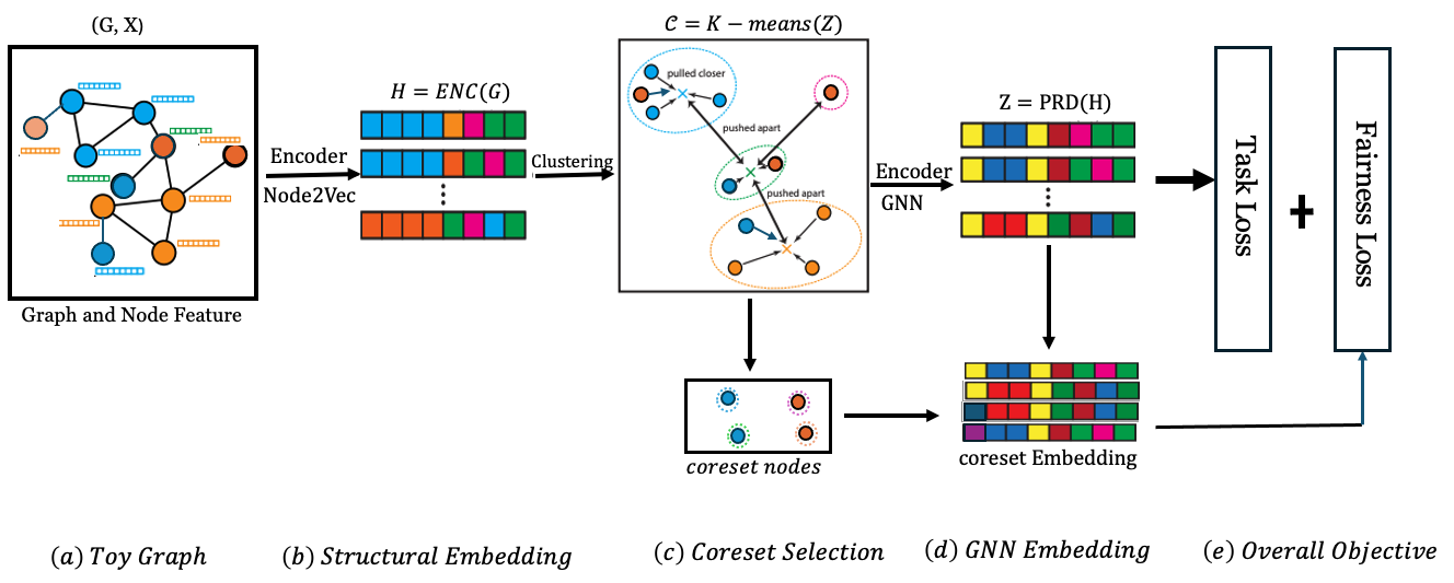
The overall framework of the ComFairGNN is illustrated in Figure 2. We first design a strategy of communities using a clustering algorithm based on structural contrast in Figure 2(c) to evaluate the effectiveness of the existing fairness methods and our proposed method at the community level. To facilitate the debiasing function, we split nodes in each community into two subgroups based on their sensitive feature and sample coreset nodes from each community based on their neighborhood homophily distribution ratio Figure 2(c). The coreset nodes contrast each other based on their output similarity to mitigate structural bias at the community level Figure 2(d). More specifically, the sampled coreset based debiasing function aims to balance the neighborhood distribution of nodes in different communities and remove bias by improving the output similarity of the nodes that have the same label. Thus, by trying to maximize the similarity of nodes in the coreset with the same label, the GNN is able to debias the neighborhood aggregation and balance the two groups. The GNN is optimized by the task loss and the coreset fairness loss Figure 2(e).
3.1. Community level Structural Contrast
To debias nodes in a community with varying label neighborhood distribution, we propose a debiasing function based on the coreset sample nodes , which are selected from different communities. Coreset selection methods aim to identify crucial subsets of training examples by employing specific heuristic criteria (Toneva et al., 2018). These subsets are considered essential for effectively training the model. Our study proposes a new method of graph coreset selection method to debias GNNs, addressing the local structural bias in their aggregation process. The coreset nodes are selected equally from each community for both groups to learn the debiasing function by contrasting between two groups of nodes, namely, subgroups and . Note that GNNs neighborhood aggregation in Eq. 1, can only access its one-hop local contexts in each layer. The majority of real-world networks of nodes in a community tend to be from the same subgroup influenced by the sensitive attribute. Thus, it is a natural choice to select the coreset sample nodes of both groups from each community to balance the structural imbalance between different communities.
| (8) |
Here indicates the coreset sample nodes for all . represents the total number of communities, and and represent selected sample nodes from subgroup and in community respectively.
To minimize the structural bias between the two groups in different communities, we contrast the output similarity of nodes with the same label in the coreset. This tends to maximize the similarity of nodes of the same label in different communities. This strategy enables GNNs to implicitly eliminate the structural bias between different communities.
3.2. Coreset Selection for GNNs Debiasing
To fundamentally eliminate the structural bias of GNNs neighborhood aggregation, which is the key operation in GNNs, we propose a neighborhood homophily distribution ratio to select the sample coreset from different communities.
Node neighborhood homophily distribution ratio: The homophily ratio in graphs is typically defined based on the similarity between connected node pairs. In this context, two nodes are considered similar if they share the same node label. The formal definition of the homophily ratio is derived from this intuition, as follows (Ma et al., 2021).
Definition 0 (Node Homophily Ratio).
For a graph with node label vector , we define the edge homophily ratio as the proportion of edges linking nodes sharing identical labels. The formal definition is as follows:
| (9) |
where is the number of neighboring edges of node in the graph and is the indicator function.
A node in a graph is generally classified as highly homophilous when its edge homophily ratio is high, typically falling within the range , assuming an appropriate label context. Conversely, a node is considered heterophilous when its edge homophily ratio is low. Here, denotes the edge homophily ratio as previously defined.
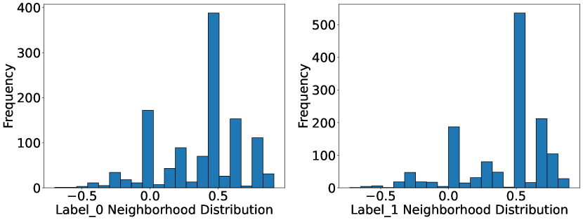
As shown in figure 3, the neighborhood distribution ratio for identical label nodes in pokec-z dataset varies largely. If we consider that all nodes that share the same label have similar initial node features, then cleary, after GNN 1-hop neighborhood aggregation, the identical label nodes will have different output embedding. This inability to differentiate the embedding space of identical nodes in different communities of the graph can potentially lead the GNN to be biased towards certain subgroups. Considering this, the debiasing coreset nodes are sampled based on their neighborhood distribution from all communities of the graph.
Fairness-aware Graph Coreset: aims to identify a representative subset of training nodes , where , along with an associated set of sample weights. This selection is designed to approximate the training loss across all , while maintaining fairness considerations. The graph coreset selection problem is formulated as:
| (10) |
which minimizes the worst-case error for all . Both the graph adjacency matrix and node feature matrix are still needed to compute the full-graph embeddings in the coreset loss. Since the goal of the fairness-aware graph, coreset is to debias the neighborhood aggregation of GNNs at the community level, we consider the coreset samples of both groups of and from all communities of the graph.
3.3. Training Objective and Constraints:
We focus on the task of node classification. We incorporate both the classification loss and the fairness loss associated with the classification to enhance the training process as illustrated in figure 2(e).
Classification loss: In node classification tasks, the Graph Neural Network (GNNs) final layer typically adapts its dimensionality to align with the number of classes. It utilizes a softmax activation function, wherein the probability of class is represented by the output dimension. To optimize the model’s parameters, we minimize the cross-entropy loss, defined as:
| (11) |
Here, denotes the number of labeled examples (rows in ), while represents the predicted probability of the example belonging to the class.
Fairness loss: As the proposed coreset selection aims to maintain fair representations across different groups, we introduce a fairness loss on the selected coreset samples . We group the samples in based on their class label. Let and denote the groups of samples in the coreset with labels and , respectively for binary classification. We use a similarity-based loss, trying to achieve parity in the average pairwise similarities for the two label groups in , as follows:
| (12) |
where is a cosine similarity function between two samples of same label. This fairness loss drives the coreset selection toward balancing the average intra-label similarities between the two label groups in . It aims to constrain the similarity distribution of labels to be similar across the two groups, and .
Overall loss: By combining all the above loss terms, we formulate the overall loss as
| (13) |
4. Experiments
We aim to address the following research questions in our experiments. RQ1: How reliable is the reported fairness score of graph debiasing methods free from paradox at a community level? RQ2: How efficient are the existing graph fairness evaluation methods in estimating the bias of GNNs at a community level? RQ3: How efficient is our proposed ComFairGNN method in terms of both accuracy and fairness at the community level?
| Dataset | Comm-Id | Comm(size) | Group_0 (size) | Group_1 (size) |
|---|---|---|---|---|
| Pokec-z | 1 | 309 | 293 | 16 |
| 2 | 282 | 26 | 256 | |
| 3 | 259 | 28 | 231 | |
| 4 | 1412 | 1019 | 393 | |
| 5 | 302 | 256 | 46 | |
| Pokec-n | 1 | 428 | 407 | 21 |
| 2 | 360 | 58 | 302 | |
| 3 | 361 | 43 | 318 | |
| 3 | 641 | 28 | 231 | |
| 4 | 389 | 322 | 67 | |
| 1 | 55 | 27 | 28 | |
| 2 | 37 | 29 | 8 | |
| 3 | 65 | 49 | 16 |
| Method | Dataset | ACC | AUC | ||||
|---|---|---|---|---|---|---|---|
| Vanilla GCN | Pokec-z | 69.29 1.72 | 69.51 2.7 | 14.43 0.7 | 12.88 0.94 | -14.43 0.7 | -12.88 0.94 |
| Pokec-n | 70.77 1.32 | 70.45 1.7 | 18.03 0.57 | 14.14 2.01 | 18.03 0.57 | 14.14 2.01 | |
| 81.53 1.52 | 61.62 2.1 | 12.73 0.7 | 12.30 1.0 | -12.73 0.7 | -12.30 1.0 | ||
| FairGNN | Pokec-z | 68.95 0.1 | 72.24 0.3 | 5.17 1.3 | 7.79 0.7 | -5.17 1.3 | -6.79 0.7 |
| Pokec-n | 69.14 0.1 | 70.18 0.3 | 4.26 1.3 | 3.87 0.7 | 4.26 1.3 | 3.87 0.7 | |
| 85.35 0.77 | 64.62 1.6 | 2.22 0.6 | 6.36 1. 0 | 2.22 0.6 | 6.36 1. 0 | ||
| NIFTY | Pokec-z | 67.34 1.51 | 67.49 1.20 | 5.89 1.32 | 5.85 0.9 | -5.89 1.32 | -5.85 0.9 |
| Pokec-n | 69.41 1.51 | 69.08 1.20 | 8.63 1.32 | 10.42 0.9 | -8.63 1.32 | -10.42 0.9 | |
| 77.07 1.28 | 73.05 1.87 | 7.88 1.0 | 8.95 1.3 | 7.88 1.0 | 8.95 1.3 | ||
| UGE | Pokec-z | 63.64 2.57 | 64.61 2.1 | 14.34 2.3 | 11.74 1.9 | -14.34 2.3 | -11.74 1.9 |
| Pokec-n | 67.48 2.72 | 66.67 2.71 | 10.34 2.3 | 12.74 1.9 | -10.34 2.3 | -12.74 1.9 | |
| 64.33 0.94 | 63.46 1.8 | 5.69 1.2 | 13.17 1.5 | 5.69 1.2 | 13.17 1.5 | ||
| ComFairGNN | Pokec-z | 70.25 0.1 | 71.11 0.3 | 0.18 1.3 | 1.00 0.7 | 0.18 1.3 | 1.00 0.7 |
| Pokec-n | 69.41 0.7 | 66.43 0.97 | 0.19 0.45 | 0.90 0.67 | -0.19 0.45 | -0.90 0.67 | |
| 85.35 0.77 | 74.62 2.6 | 3.96 0.6 | 7.63 1. 0 | 3.96 0.6 | 7.63 1. 0 |
| Method | Comm-Id | ACC | AUC | ||||
|---|---|---|---|---|---|---|---|
| Vanilla GCN | 1 | 62.36 | 57.89 | 45.38 | 21.36 | -45.38 | -21.36 |
| 2 | 76.84 | 71.67 | 7.32 | 10.34 | 7.32 | 10.34 | |
| 3 | 64.73 | 63.85 | 14.97 | 12.59 | 14.97 | 12.59 | |
| 4 | 72.00 | 72.24 | 11.38 | 4.14 | 11.38 | 4.14 | |
| 5 | 84.43 | 74.76 | 10.66 | 0.64 | 10.66 | 0.64 | |
| FairGNN | 1 | 61.34 | 56.56 | 2.81 | 9.67 | 2.81 | -9.67 |
| 2 | 75.71 | 71.58 | 7.23 | 7.97 | -7.23 | -7.97 | |
| 3 | 61.43 | 60.26 | 21.19 | 18.21 | 21.19 | 18.21 | |
| 4 | 69.14 | 69.36 | 11.76 | 13.29 | -11.76 | -13.29 | |
| 5 | 79.24 | 66.35 | 13.18 | 6.22 | 13.18 | 6.22 | |
| NIFTY | 1 | 61.56 | 56.46 | 1.31 | 4.69 | 1.31 | -4.69 |
| 2 | 77.97 | 70.74 | 13.45 | 14.68 | -13.45 | -14.68 | |
| 3 | 61.63 | 60.00 | 9.77 | 14.14 | 9.77 | 14.14 | |
| 4 | 68.57 | 66.67 | 5.16 | 4.62 | -5.16 | -4.62 | |
| 5 | 79.93 | 63.56 | 13.74 | 11.16 | 13.74 | 11.16 | |
| UGE | 1 | 60.88 | 51.71 | 21.29 | 27.68 | -21.29 | -27.68 |
| 2 | 69.49 | 61.91 | 10.42 | 2.72 | -10.42 | -2.72 | |
| 3 | 61.24 | 58.91 | 1.23 | 11.91 | 1.23 | 11.91 | |
| 4 | 58.48 | 61.34 | 51.89 | 60.50 | -51.89 | -60.50 | |
| 5 | 78.55 | 62.69 | 3.77 | 6.00 | -3.77 | -6.00 | |
| ComFairGNN | 1 | 74.43 | 72.97 | 5.63 | 1.04 | -5.63 | -1.04 |
| 2 | 73.44 | 75.98 | 7.21 | 0.07 | 7.21 | 0.07 | |
| 3 | 72.97 | 73.26 | 3.46 | 1.90 | 3.46 | 1.90 | |
| 4 | 72.97 | 65.44 | 2.59 | 3.40 | -2.59 | -3.40 | |
| 5 | 76.67 | 74.05 | 2.61 | 1.08 | 2.61 | 1.08 |
| Method | Comm-Id | ACC | AUC | ||||
|---|---|---|---|---|---|---|---|
| Vanilla GCN | 1 | 72.30 | 73.73 | 15.20 | 6.72 | -15.20 | -6.72 |
| 2 | 69.19 | 68.00 | 13.06 | 2.74 | 13.06 | 2.74 | |
| 3 | 66.11 | 59.05 | 26.67 | 14.32 | -26.67 | -14.32 | |
| 4 | 71.39 | 71.96 | 8.29 | 6.16 | 8.29 | 6.16 | |
| 5 | 68.42 | 66.25 | 19.14 | 8.86 | 19.14 | 8.86 | |
| FairGNN | 1 | 65.68 | 64.42 | 22.65 | 12.27 | 22.65 | 12.27 |
| 2 | 63.17 | 62.71 | 9.67 | 9.43 | 9.67 | 9.43 | |
| 3 | 58.68 | 55.46 | 16.35 | 17.85 | -16.35 | -17.85 | |
| 4 | 74.89 | 62.42 | 10.60 | 8.57 | 10.60 | 8.57 | |
| 5 | 60.23 | 57.35 | 4.20 | 4.76 | -4.20 | -4.76 | |
| NIFTY | 1 | 72.97 | 72.19 | 23.17 | 29.61 | 23.17 | 29.61 |
| 2 | 67.23 | 66.10 | 4.29 | 1.54 | 4.29 | 1.54 | |
| 3 | 66.39 | 58.59 | 9.44 | 1.59 | -9.44 | 1.59 | |
| 4 | 79.65 | 68.73 | 8.29 | 8.09 | 8.29 | 8.09 | |
| 5 | 69.59 | 67.68 | 7.34 | 14.19 | -7.34 | -14.19 | |
| UGE | 1 | 62.70 | 61.14 | 33.67 | 6.36 | 33.67 | 6.36 |
| 2 | 63.73 | 62.45 | 15.82 | 18.03 | 15.82 | 18.03 | |
| 3 | 64.71 | 55.57 | 37.78 | 30.09 | -37.78 | -30.09 | |
| 4 | 73.16 | 59.70 | 7.08 | 4.41 | -7.08 | -4.41 | |
| 5 | 57.31 | 55.75 | 20.89 | 2.86 | 20.89 | 2.86 | |
| ComFairGNN | 1 | 66.82 | 61.88 | 11.65 | 4.00 | 11.65 | 4.00 |
| 2 | 70.56 | 70.87 | 3.16 | 1.75 | -3.16 | -1.75 | |
| 3 | 65.62 | 65.67 | 0.17 | 2.40 | -0.17 | -2.40 | |
| 4 | 72.49 | 64.41 | 8.59 | 5.45 | -8.59 | -5.45 | |
| 5 | 69.4 | 70.16 | 1.75 | 1.24 | 1.75 | 1.24 |
| Method | Comm-Id | ACC | AUC | ||||
|---|---|---|---|---|---|---|---|
| Vanilla GCN | 1 | 83.02 | 54.42 | 5.26 | 8.33 | 5.26 | 8.33 |
| 2 | 72.97 | 68.59 | 23.53 | 21.98 | -23.53 | -21.98 | |
| 3 | 85.07 | 54.55 | 1.49 | 4.55 | .49 | 4.55 | |
| FairGNN | 1 | 94.83 | 49.11 | 5.26 | 5.00 | 5.26 | 5.00 |
| 2 | 70.00 | 62.50 | 1.10 | 20.57 | -1.10 | 20.57 | |
| 3 | 84.06 | 57.46 | 5.00 | 6.96 | 5.00 | 6.96 | |
| NIFTY | 1 | 81.82 | 50.00 | 0.00 | 0.00 | 0.00 | 0.00 |
| 2 | 67.57 | 56.68 | 24.68 | 29.31 | 24.68 | 29.31 | |
| 3 | 78.46 | 52.59 | 2.56 | 4.21 | -2.56 | 4.21 | |
| UGE | 1 | 76.36 | 62.22 | 3.36 | 13.87 | 3.36 | 13.87 |
| 2 | 36.36 | 50.00 | 3.78 | 4.14 | 3.78 | 4.14 | |
| 3 | 68.12 | 50.58 | 0.99 | 4.83 | -0.99 | 4.83 | |
| ComFairGNN | 1 | 81.78 | 77.12 | 2.43 | 4.75 | 2.43 | 4.75 |
| 2 | 63.41 | 52.61 | 2.51 | 1.76 | -2.51 | -1.76 | |
| 3 | 81.13 | 50.00 | 0.09 | 0.01 | 0.09 | 0.01 |
4.1. Experimental Setup and Datasets
Datasets. In this context, the downstream task is node classification. We conducted our experiments using three real-world datasets: Pokec-z, Pokec-n, and Facebook. Specifically, Pokec-z and Pokec-n datasets are derived from Pokec, a well-known social network in Slovakia (Takac and Zabovsky, 2012). This dataset encompasses anonymized information from the entire network. Due to its extensive size, the authors in (Dai and Wang, 2021) extracted two subsets from the original Pokec dataset, designated as Pokec-z and Pokec-n, based on users’ provincial affiliations. In the dataset, each user is represented as a node, and each edge represents a friendship between two users. The sensitive attribute in this context is the users’ location. The objective is to classify users based on their field of work. The Facebook dataset is derived from the Facebook DataSet (He and McAuley, 2016). In this dataset, each user is represented as a node, and each edge signifies a friendship between two users. The sensitive attribute is the gender information associated with each node. We summarize the datasets in Table 6
| Dataset | Nodes | Edges | Features | Classes |
|---|---|---|---|---|
| Pokec-z | 67,796 | 882,765 | 276 | 2 |
| Pokec-n | 66,569 | 198,353 | 265 | 2 |
| 1,034 | 26,749 | 573 | 2 |
Baseline Methods: We investigate the effectiveness of four state-of-the-art GNN debiasing methods at a community level, namely FairGNN (Dai and Wang, 2021), NIFTY (uNIfying Fairness and stabiliTY) (Agarwal et al., 2021a), and UGE (Wang et al., 2022a). FairGNN utilizes adversarial training to eliminate sensitive attribute information from node embeddings. NIFTY improves fairness by aligning predictions based on both perturbed and unperturbed sensitive attributes. This approach generates graph counterfactuals by inverting the sensitive feature values for all nodes while maintaining all other attributes. The method then incorporates a regularization term in the loss function to promote similarity between node embeddings derived from the original graph and its counterfactual counterpart. UGE derives node embeddings from a neutral graph that is free of biases and unaffected by sensitive node attributes, addressing the issue of unbiased graph embedding. We use GCN (Kipf and Welling, 2016) as the backbone GNN model.
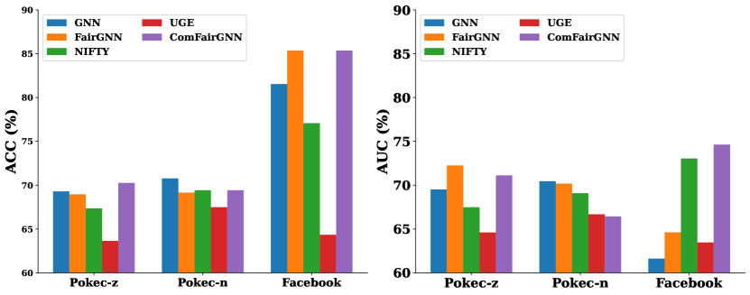
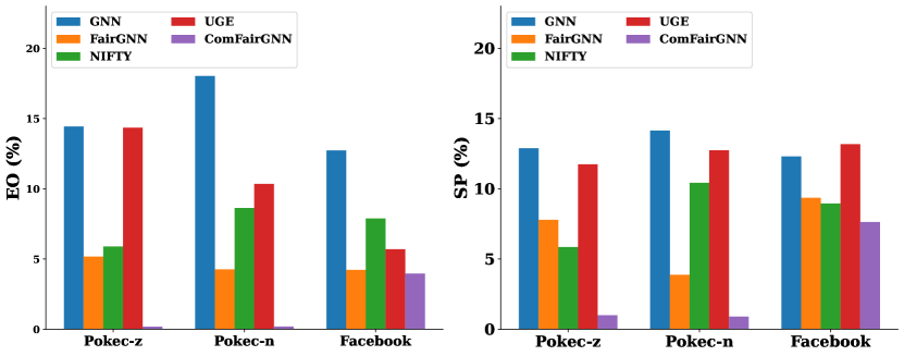
Evaluation: We use the widely adopted group fairness metrics, SP (Statistical Parity), and EO (Equal Opportunity) to evaluate fairness at a community level in Tables 3, 4, 5 and graph level in Table 2. As discussed in section 2.3, SP and EO fundamentally require that the model’s outcomes remain statistically independent of the nodes’ sensitive features. In particular, we form two groups of nodes from the test set, and , containing test nodes with sensitive features and , respectively. The two groups fairness is the most serious fairness issue in GNN’s tasks. As GNNs learn by neighborhood aggregation section 2.1, we evaluate fairness within different subgraphs or communities within the larger graph. This can help identify and address local disparities more effectively. We select and nodes within the community to evaluate the model’s disparity locally, which may present more prominent biases. We select top and bottom sample homophily neighborhood distribution ratio from each community to formulate the representative coreset nodes from the training set during training. These nodes are sufficient to cover the local contextual structures where biases are rooted. To further conduct a comprehensive fairness evaluation, we additionally select coreset nodes from both extremes of the homophily neighborhood distribution ratio, specifically choosing nodes from the top and bottom and of this distribution. For evaluating model performance on the node classification task, we use classification accuracy ACC and the area under the receiver operating characteristic curve AUC.
Implementation Setup: For a fair comparison with other baseline methods, we employ a standard Graph Convolutional Network (GCN) (Kipf and Welling, 2016) as our encoder. This choice emphasizes our focus on the overall framework. Consistency is maintained across all baselines, which also utilize GCN layers.We implement two-layer GCNs for all datasets and incorporate a two-layer Multilayer Perceptron (MLP) for the predictor network. Our model is implemented using PyTorch and PyTorch Geometric, leveraging their efficient graph processing capabilities. The baseline implementations were adopted from the official PyGDebias (Dong et al., 2023) graph fairness library. Each method was run for three iterations, using the best hyperparameters reported in the original paper. We Perform for epochs with a learning rate on each dataset on the node classification task for three iterations. All of our experiments were conducted on 16 GB NVIDIA V100 GPUs.
Fairness Paradoxes: To address RQ1, we evaluate the effectiveness of current debiasing techniques for GNNs at the community level and compare the consistency of their debiasing performance when applied to the entire graph. We first measure the group fairness of the GCN model with the debiasing method applied to the original input graph . Next, we measure the group fairness of the same GCN model with the debiasing method applied at the community level. We use the group fairness metrics and . We observe that the fairness performance across the communities is not as consistent as the fairness score reported for the entire graph across all three real-world datasets for all methods. For example, in Table 3, we observe that the unfairness estimation for the Pokec-z dataset using and is higher for communities {2, 3, 4, 5} compared to and for the entire dataset when FairGNN debiasing method is used. We also observed Simpson’s paradox on Pokec-z with UGE: the accuracy of Group_ (66.06) is higher than Group_ (62.36) on the entire graph, but on the community level, for 4 out of 5 communities, predictions on Group_ have better accuracy.
Over-Simplification of Fairness Evaluation: It is important to note that both and group fairness metrics use absolute values for their numerical results. measures whether different groups have equal true positive rates. Using absolute values might mask local disparities. For example, in one part of the graph, one group might have a very high true positive rate, while in another part, the same group might have a very low rate. An absolute measure could average these out, hiding the local unfairness as indicated in the results of (without absolute value) for different communities; some are positive while others are negative. Similarly, checks if different groups have the same likelihood of being assigned a positive outcome. the absolute values could hide local variations in dominance. A group might have equal overall positive outcomes when averaged out, but locally, one group might be consistently favored or disfavored as indicated in the results without absolute value . Therefore, if one part of the graph is very fair and another is very unfair, the overall metric might show moderate fairness. This is misleading because it does not reflect the lived experiences of individuals in the unfair part of the graph.
4.2. Model Analysis
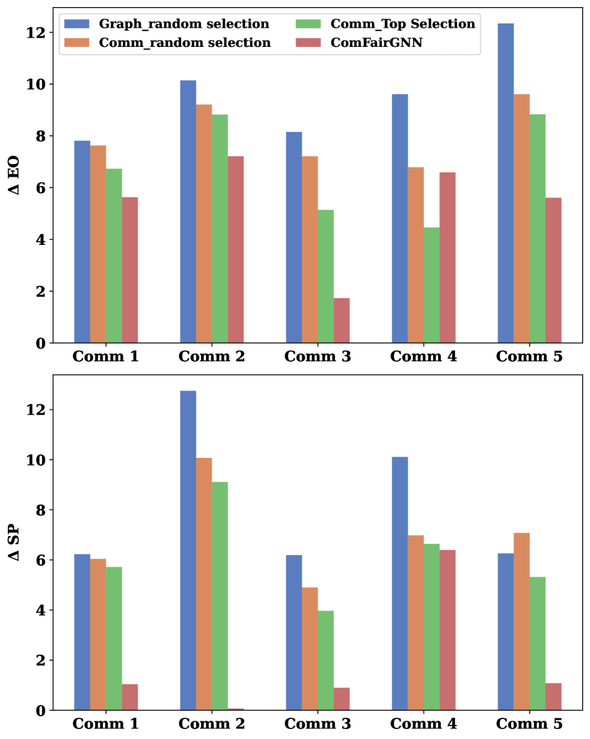
Ablation Study: To Validate the coreset section of ComFairGNN, we consider different variants of selection approaches based on their homophily neighborhood distribution, section 3.2. (1) Random node selection: we select an equal number of coreset nodes from groups and of the entire train set. (2) Top homophily neighborhood ratio distribution: we select the top highly homophily nodes of both groups and from each community. (3) we select number of coreset nodes of both groups and from each community randomly. We report the result in figure 6 and make several observations. Firstly, without selecting the coreset nodes from both extremes of homophily ratio distribution, we often get worse fairness performance, which means representative nodes from both high and low homophily ratio distribution can mitigate the structural bias at the community level. Secondly, by selecting the coreset nodes randomly from the entire train set, the fairness metric generally becomes worse. Thus, selecting the coreset at the community level is effective in driving the debiasing context at the local subgraph
5. Related Work
5.1. Fairness in Graph
Fairness in Graph Neural Networks (GNNs) is an emerging area of research, researchers have performed signifi- cant work to measure the fairness of those systems(Wang et al., 2019; Fan et al., 2021; li2021user; Kleindessner et al., 2019; Horowitz and Kamvar, 2010). Generally, fairness can be categorized into group fairness and individual fairness. Group fairness focuses on ensuring that the model does not make decisions that favor or disadvantage certain groups. Group fairness is one of the mainly studied. EDITS (Dong et al., 2022) modifies the adjacency matrix and node attributes to produce unbiased graph-structured data by reducing the Wasserstein distance between different groups. Additionally, some studies (Dai and Wang, 2021; Wang et al., 2022b) achieve fairness in GNNs through adversarial training, resulting in a model that generates node embeddings indistinguishable with respect to the sensitive attribute. FairGNN (Dai and Wang, 2021) incorporates fairness regularization to address bias in graph-based tasks. It aims to ensure equitable treatment of different groups in both learned representations and final predictions. UGE (Wang et al., 2022a) addresses the unbiased graph embedding problem by learning node representations from a bias-free underlying graph. This approach eliminates the influence of sensitive node attributes on the embedding process. Another aspect of fairness, often referred to as counterfactual fairness, ensures that changes in sensitive attributes do not impact the prediction results (Agarwal et al., 2021a). NIFTY (Agarwal et al., 2021b) enhances counterfactual fairness and stability in node representations through a novel triplet-based objective function. It employs layer-wise weight normalization using the Lipschitz constant to improve performance and reliability. GEAR addresses graph unfairness through counterfactual graph augmentation and adversarial learning for attribute-insensitive embeddings. These combined approaches effectively reduce bias in graph-based models. GEAR (Ma et al., 2022) addresses graph unfairness through counterfactual graph augmentation and adversarial learning for attribute-insensitive embeddings. These combined approaches effectively reduce bias in graph-based models. Deg-FairGNN (Liu et al., 2023) aims to ensure fair outcomes for nodes with varying degrees within a group. Despite they introduce attribute and structural group fairness, overlooked the inherent local structural bias. In terms of individual fairness, nodes sharing similar attributes are treated equivalently (Dong et al., 2021). For example, REDRESS (Dong et al., 2021) proposes a ranking-based individual fairness optimization method to encourage each individual node relative similarity ranking list to the other nodes during the input and output. InFoRM (Kang et al., 2020) assesses GNN individual fairness using node similarity matrices. It incorporates a modified (d1, d2)-Lipschitz property to address fairness challenges in interconnected graph structures, moving beyond node features alone. However, none of these works are designed for community-level fairness on graphs.
5.2. Detecting Fairness Paradox
There have been prior works that study the fairness paradoxes due to historical bias using statistical measures of fairness and counterfactual fairness. Counterfactual fairness (Kusner et al., 2017) introduces a path-specific causal effect on the prediction outcomes in discrimination analysis. The study demonstrates the paradox that arises when removing the sensitive attribute to achieve fairness; elements of the input feature can still contain discriminatory information that may not be immediately apparent. (Prost et al., 2022) demonstrates Simpson’s Paradox in the context of recommender system fairness, showing that the aggregate metric of fairness is influenced by differences in user distribution across the subgroups.
6. Conclusion
In this paper, we investigate the effectiveness of existing graph debiasing methods and the fairness evaluation paradoxes at the community level. We first group the nodes of the graph into communities based on their structural similarities, then assess the fairness of GNNs with debiasing methods for different demographic subgroups. Our findings demonstrate fairness inconsistencies and paradoxes across various graph communities. By removing the absolute values in and , we show that absolute measures might dilute these effects, leading to an underestimation of bias in specific communities within the large graph. To address the community-level bias inherent in GNN neighborhood aggregation, we introduce ComFairGNN, a novel fairness-aware GNN framework compatible with various neighborhood aggregation-based GNN architectures. Our approach targets local structural bias by modulating representative coreset nodes from diverse communities through embedding similarity contrast. Comprehensive experiments on three benchmark datasets demonstrate ComFairGNN’s efficacy, yielding promising results in both accuracy and fairness metrics.
References
- (1)
- Agarwal et al. (2021a) Chirag Agarwal, Himabindu Lakkaraju, and Marinka Zitnik. 2021a. Towards a unified framework for fair and stable graph representation learning. In Uncertainty in Artificial Intelligence. PMLR, 2114–2124.
- Agarwal et al. (2021b) Chirag Agarwal, Himabindu Lakkaraju*, and Marinka Zitnik*. 2021b. Towards a Unified Framework for Fair and Stable Graph Representation Learning. (2021).
- Blyth (1972) Colin R Blyth. 1972. On Simpson’s paradox and the sure-thing principle. J. Amer. Statist. Assoc. 67, 338 (1972), 364–366.
- Bourigault et al. (2014) Simon Bourigault, Cedric Lagnier, Sylvain Lamprier, Ludovic Denoyer, and Patrick Gallinari. 2014. Learning social network embeddings for predicting information diffusion. In Proceedings of the 7th ACM international conference on Web search and data mining. 393–402.
- Dai and Wang (2021) Enyan Dai and Suhang Wang. 2021. Say no to the discrimination: Learning fair graph neural networks with limited sensitive attribute information. In Proceedings of the 14th ACM International Conference on Web Search and Data Mining. 680–688.
- Dong et al. (2021) Yushun Dong, Jian Kang, Hanghang Tong, and Jundong Li. 2021. Individual fairness for graph neural networks: A ranking based approach. In Proceedings of the 27th ACM SIGKDD Conference on Knowledge Discovery & Data Mining. 300–310.
- Dong et al. (2022) Yushun Dong, Ninghao Liu, Brian Jalaian, and Jundong Li. 2022. Edits: Modeling and mitigating data bias for graph neural networks. In Proceedings of the ACM web conference 2022. 1259–1269.
- Dong et al. (2023) Yushun Dong, Jing Ma, Song Wang, Chen Chen, and Jundong Li. 2023. Fairness in graph mining: A survey. IEEE Transactions on Knowledge and Data Engineering (2023).
- Dwork et al. (2012) Cynthia Dwork, Moritz Hardt, Toniann Pitassi, Omer Reingold, and Richard Zemel. 2012. Fairness through awareness. In Proceedings of the 3rd innovations in theoretical computer science conference. 214–226.
- Fan et al. (2021) Wei Fan, Kunpeng Liu, Rui Xie, Hao Liu, Hui Xiong, and Yanjie Fu. 2021. Fair graph auto-encoder for unbiased graph representations with wasserstein distance. In 2021 IEEE International Conference on Data Mining (ICDM). IEEE, 1054–1059.
- Gölz et al. (2019) Paul Gölz, Anson Kahng, and Ariel D Procaccia. 2019. Paradoxes in fair machine learning. Advances in Neural Information Processing Systems 32 (2019).
- Grover and Leskovec (2016) Aditya Grover and Jure Leskovec. 2016. node2vec: Scalable feature learning for networks. In Proceedings of the 22nd ACM SIGKDD international conference on Knowledge discovery and data mining. 855–864.
- Guerra et al. (2013) Pedro Guerra, Wagner Meira Jr, Claire Cardie, and Robert Kleinberg. 2013. A measure of polarization on social media networks based on community boundaries. In Proceedings of the international AAAI conference on web and social media, Vol. 7. 215–224.
- Hardt et al. (2016) Moritz Hardt, Eric Price, and Nati Srebro. 2016. Equality of opportunity in supervised learning. Advances in neural information processing systems 29 (2016).
- He and McAuley (2016) Ruining He and Julian McAuley. 2016. Ups and downs: Modeling the visual evolution of fashion trends with one-class collaborative filtering. In proceedings of the 25th international conference on world wide web. 507–517.
- Horowitz and Kamvar (2010) Damon Horowitz and Sepandar D Kamvar. 2010. The anatomy of a large-scale social search engine. In Proceedings of the 19th international conference on World wide web. 431–440.
- Kamishima and Akaho (2017) Toshihiro Kamishima and Shotaro Akaho. 2017. Considerations on recommendation independence for a find-good-items task. (2017).
- Kang et al. (2020) Jian Kang, Jingrui He, Ross Maciejewski, and Hanghang Tong. 2020. Inform: Individual fairness on graph mining. In Proceedings of the 26th ACM SIGKDD international conference on knowledge discovery & data mining. 379–389.
- Kipf and Welling (2016) Thomas N Kipf and Max Welling. 2016. Semi-supervised classification with graph convolutional networks. arXiv preprint arXiv:1609.02907 (2016).
- Kleindessner et al. (2019) Matthäus Kleindessner, Samira Samadi, Pranjal Awasthi, and Jamie Morgenstern. 2019. Guarantees for spectral clustering with fairness constraints. In International Conference on Machine Learning. PMLR, 3458–3467.
- Kusner et al. (2017) Matt J Kusner, Joshua Loftus, Chris Russell, and Ricardo Silva. 2017. Counterfactual fairness. Advances in neural information processing systems 30 (2017).
- Lambrecht and Tucker (2019) Anja Lambrecht and Catherine Tucker. 2019. Algorithmic bias? An empirical study of apparent gender-based discrimination in the display of STEM career ads. Management science 65, 7 (2019), 2966–2981.
- Liu et al. (2023) Zemin Liu, Trung-Kien Nguyen, and Yuan Fang. 2023. On Generalized Degree Fairness in Graph Neural Networks. arXiv preprint arXiv:2302.03881 (2023).
- Ma et al. (2022) Jing Ma, Ruocheng Guo, Mengting Wan, Longqi Yang, Aidong Zhang, and Jundong Li. 2022. Learning fair node representations with graph counterfactual fairness. In Proceedings of the Fifteenth ACM International Conference on Web Search and Data Mining. 695–703.
- Ma et al. (2021) Yao Ma, Xiaorui Liu, Neil Shah, and Jiliang Tang. 2021. Is homophily a necessity for graph neural networks? arXiv preprint arXiv:2106.06134 (2021).
- MacQueen et al. (1967) James MacQueen et al. 1967. Some methods for classification and analysis of multivariate observations. In Proceedings of the fifth Berkeley symposium on mathematical statistics and probability, Vol. 1. Oakland, CA, USA, 281–297.
- Nickel et al. (2015) Maximilian Nickel, Kevin Murphy, Volker Tresp, and Evgeniy Gabrilovich. 2015. A review of relational machine learning for knowledge graphs. Proc. IEEE 104, 1 (2015), 11–33.
- Prost et al. (2022) Flavien Prost, Ben Packer, Jilin Chen, Li Wei, Pierre Kremp, Nicholas Blumm, Susan Wang, Tulsee Doshi, Tonia Osadebe, Lukasz Heldt, et al. 2022. Simpson’s Paradox in Recommender Fairness: Reconciling differences between per-user and aggregated evaluations. arXiv preprint arXiv:2210.07755 (2022).
- Rahman et al. (2019) Tahleen Rahman, Bartlomiej Surma, Michael Backes, and Yang Zhang. 2019. Fairwalk: Towards fair graph embedding. (2019).
- Saxena et al. (2022) Akrati Saxena, George Fletcher, and Mykola Pechenizkiy. 2022. HM-EIICT: Fairness-aware link prediction in complex networks using community information. Journal of Combinatorial Optimization 44, 4 (2022), 2853–2870.
- Shiao et al. (2023) William Shiao, Uday Singh Saini, Yozen Liu, Tong Zhao, Neil Shah, and Evangelos E Papalexakis. 2023. Carl-g: Clustering-accelerated representation learning on graphs. In Proceedings of the 29th ACM SIGKDD Conference on Knowledge Discovery and Data Mining. 2036–2048.
- Takac and Zabovsky (2012) Lubos Takac and Michal Zabovsky. 2012. Data analysis in public social networks. In International scientific conference and international workshop present day trends of innovations, Vol. 1.
- Toneva et al. (2018) Mariya Toneva, Alessandro Sordoni, Remi Tachet des Combes, Adam Trischler, Yoshua Bengio, and Geoffrey J Gordon. 2018. An empirical study of example forgetting during deep neural network learning. arXiv preprint arXiv:1812.05159 (2018).
- Veličković et al. (2017) Petar Veličković, Guillem Cucurull, Arantxa Casanova, Adriana Romero, Pietro Lio, and Yoshua Bengio. 2017. Graph attention networks. arXiv preprint arXiv:1710.10903 (2017).
- von Kügelgen et al. (2021) Julius von Kügelgen, Luigi Gresele, and Bernhard Schölkopf. 2021. Simpson’s paradox in Covid-19 case fatality rates: a mediation analysis of age-related causal effects. IEEE transactions on artificial intelligence 2, 1 (2021), 18–27.
- Wang et al. (2019) Daixin Wang, Jianbin Lin, Peng Cui, Quanhui Jia, Zhen Wang, Yanming Fang, Quan Yu, Jun Zhou, Shuang Yang, and Yuan Qi. 2019. A semi-supervised graph attentive network for financial fraud detection. In 2019 IEEE International Conference on Data Mining (ICDM). IEEE, 598–607.
- Wang et al. (2022a) Nan Wang, Lu Lin, Jundong Li, and Hongning Wang. 2022a. Unbiased graph embedding with biased graph observations. In Proceedings of the ACM Web Conference 2022. 1423–1433.
- Wang et al. (2022b) Yu Wang, Yuying Zhao, Yushun Dong, Huiyuan Chen, Jundong Li, and Tyler Derr. 2022b. Improving fairness in graph neural networks via mitigating sensitive attribute leakage. In Proceedings of the 28th ACM SIGKDD conference on knowledge discovery and data mining. 1938–1948.
- Wu et al. (2019) Jun Wu, Jingrui He, and Jiejun Xu. 2019. Net: Degree-specific graph neural networks for node and graph classification. In Proceedings of the 25th ACM SIGKDD international conference on knowledge discovery & data mining. 406–415.
- Xu et al. (2018) Chenguang Xu, Sarah M Brown, and Christan Grant. 2018. Detecting Simpson’s paradox. In The Thirty-First International Flairs Conference.