Comfortability of quantum walks on embedded graphs on surfaces

Yusuke Higuchi¹, Etsuo Segawa²
¹Department of Mathematics, Gakushuin University,
Tokyo 171-8588, Japan
²Graduate School of Environment and Information Sciences, Yokohama National University,
Hodogaya, Yokohama 240-8501, Japan

Abstract. In this paper, a quantum walk model which reflects the underlying embedding on the surface is proposed. We obtain the scattering matrix of this quantum walk model characterized by the faces on the surface, and find a detection of the orientablility of the underlying embedding by the scattering information. The comfortability is the square norm of the stationary state restricted to the internal and reflected by the underlying embedding. We find that quantum walker feels more comfortable to a surface with small genus in some natural setting.

Key words and phrases. Discrete-time quantum walk, graph embedding on closed surfaces, stationary state, scattering matrix, comfortability

1 Introduction

How is the underlying geometric structure estimated by a reaction to an input? To tackle this inverse problem, we adopt a discrete-time quantum walk model, and try to extract a topological structure of graphs from the behavior of the quantum superposition. Among a lot of discrete-time quantum walk models [11], the Grover walk [19] may come to mind first. In fact, using the commutativity of the Grover matrix with any permutation matrix, the time evolution of the Grover walk is easily constructed [12], which exhibits interesting behaviors [9, 10] and also plays the key roles in the quantum search [17]. Moreover there are several important properties in the Grover walk connecting to not only a random walk[QCcoupling2, 2] but also the stationary Shrödinger equation [7].

Here, let us first apply the Grover walk as a discrete-time quantum walk model and focus on the embedding of graphs on surfaces as a geometric structure. For example, the complete graph with $4$ vertices $K_{4}$ has $11$ kinds of embedding way; see Figure 7. We expect that the quantum walk “feels” these underlying embeddings. Grover walk may decide whether an underlying graph admits a topological embedding on a given surface [3]. On the other hand, the time evolution of Grover walk depends only on the adjacent structure of the underlying graph because the time evolution operator $U_{Grover}$ acts as

U_{\mathrm{Grover}}\delta_{e}=\left(\frac{2}{\mathrm{deg}(t(e))}-1\right)\delta_{\bar{e}}+\frac{2}{\mathrm{deg}(t(e))}\sum_{\epsilon:\;o(\epsilon)=t(e),\neq\bar{e}}\delta_{\epsilon},

for any standard base labeled by an arc $e$ of the underlying graph. Here $o(e)$ and $t(e)$ are origin and terminal vertices of the arc $e$ , and $\mathrm{deg}(x)$ is the degree of the vertex $x$ . Then the weights associated with transmitting and reflecting at vertex $x$ are $2/\mathrm{deg}(x)$ and $2/\deg(x)-1$ in the Grover walk, which is independent of the underlying embedding. Therefore the Grover walk can not distinguish any two embedded surfaces of a graph. Thus for our object, we need to propose another kind of discrete-time quantum walk model for this problem.

To this end, let us introduce the idea of the drawing a graph without crossings of edges and extra faces on some closed surface, which is called the two-cell embedding [6, 14, 15]. More details are given in Section 3. See also Figures 5, 6 and 7. It is well known that the two-cell embedding on a closed surface of a graph $G=(X,E)$ is realized by the rotation system [6, 14, 15]. Here $X$ and $E$ are the set of vertices and the set ofunoriented edges. The rotation system is the triple of the symmetric digraph $G=(X,A)$ , the rotation $\rho:A\to A$ and the twist $\tau:A\to\mathbb{Z}_{2}$ , where $A$ is the set of the symmetric arcs induced by $E$ . Here the rotation $\rho$ is decomposed into cyclic permutations with respect to the incoming arcs of each vertex. Thus our target can be switched to how a quantum walk model is constructed for given rotation system $(G,\rho,\tau)$ .

In this paper, the abstract graph $G$ is deformed so that information of $\rho,\tau$ are reflected and also the in- and out- degrees are equally $2$ . The regularity of the degree $2$ derives from the implementation by some optical polarizers elements [13]. See Sections 4.1, 4.2 for more detailed construction and also Figure 8. Such a new graph $G(\rho,\tau)$ is obtained by replacing each vertex of the double covering graph [6, 14] induced by $\tau$ with a directed cycle induced by $\rho$ . The replaced directed cycles are called islands, and the symmetric arcs between the islands, which reflects the original adjacent relation, are called the bridges. The tails, which are semi-infinite paths, are inserted into all the island arcs. Such an assignment of tails is called the hedgehog; see Figure 8 (d). Let us explain the time evolution below; see Sections 4.3 and 4.4 for more detail. The degree- $2$ regularity of the new graph makes it possible that the one-step time evolution on the whole space can be described by the local scattering at each vertex of the internal graph by the $2\times 2$ unitary matrix

C=\begin{bmatrix}a&b\\ c&d\end{bmatrix}.

Here $a,b,c,d$ are the complex valued weights associated with moving of a quantum walk for one step “from an island to the same island”, “ a bridge to an island”, “an island to a bridge” and “a bridge to the inverse bridge”, respectively. This unitarity of the local coin matrix $C$ includes also the unitarty of the total time evolution operator. On the other hand, we set that the dynamics on the tail is free; see (4.16) for the detailed dynamics of the free. The initial state is set so that the internal graph receives the constant inflow at every time step. If a quantum walker goes out to the external, it never come back to the internal because of the free dynamics of the tails. Such a quantum walker can be regarded as the outflow. By the balance between the in- and out- flows, this quantum walk model converges to a fixed point in the long time limit [4, 5, 8].

Now, for a fixed abstract graph $G_{o}$ , let us vary the embedding that underlies it. For every $\rho$ and $\tau$ , set $\psi_{\infty}$ as the stationary state and $\psi_{\infty}|_{G_{o}}$ as the restriction of $\psi_{\infty}$ to the internal graph $G_{o}$ . In this paper, we focus on extracting embedding structures of a graph from the stationary state of this quantum walk model. To this end, we divide the stationary state into external and internal parts; we characterize the external part by the scattering matrix, which shows a reaction of the internal graph to an input at the tails, while the internal part by the comfortability, which is corresponding to the energy in the internal graph. We estimate how quantum walker

(i) gives a scattering on the underlying embedding by finding the expression of the scattering matrix

\boldsymbol{\beta}_{out}=S\boldsymbol{\alpha}_{in},

where $S$ is independent of inflow $\boldsymbol{\alpha}_{in}$ and outflow $\boldsymbol{\beta}_{out}$ and a unitary operator [4, 5], and

(ii) feels comfortable to the embedding by defining

\mathcal{E}(G_{o},\rho,\tau):=\mathcal{E}:=\frac{1}{2}||\;\psi_{\infty}|_{G_{o}}\;||^{2},

that is, the larger $\mathcal{E}$ is, the more comfortable quantum walker feels to the underlying embedding.

Throughout this paper, in addition to the hedgehog tail condition, we subject the following assumption (2).

Assumption 1.

(1)

the assignment of tails is the hedgehog;
(2)

the $(2,2)$ element of $C$ $(=d)$ is a real number.

Under such a construction of the quantum walk reflecting the underlying embedding on a closed surface, in this paper, now we are ready to state our main result on the scattering and comfortablity.

Theorem 1.1 (Scattering).

Assume $d\in\mathbb{R}$ and set $\omega=-\det C$ and the hedgehog assignment of tails. Let $F$ be the set of faces induced by the rotation system $(G,\rho,\tau)$ . The scattering matrix is decomposed into the following $|F|$ unitary matrices as follows:

S=\bigoplus_{f\in F}S_{f},

where

S_{f}=bc\omega P_{f}\;(I_{f}-a\omega P_{f})^{-1}+dI_{f}.

Here the operators induced by each face $f$ , $I_{f}$ is the identity operator and $P_{f}$ are defined in (6.26).

Theorem 6.1 in Section 6 gives the scattering matrix in a more general setting. The operator $P_{f}$ is a weighted permutation matrix induced by the closed walk along the boudary of the face $f$ , which is called the facial walk of $f$ . The rotation system $(G,\rho,\tau)$ determines the set of faces $F$ and gives uniquely orientation of the closed walk along the boundary of the face $f\in F$ . This closed walk corresponds to the facial walk, which is expressed by a sequence of arcs, and we simply write $f$ for this closed walk. We should remark $\bar{f}\not\in F$ for $f\in F$ , where $\bar{f}$ is the inverse direction of $f$ . The weight is determined by each edge type which is passed through the facial walk. Then using this property of the scattering matrix, the detection of the orientability by the scattering information is proposed in Theorem 6.2.

Theorem 1.2 (Comfortability).

Let $G=(X,A)$ and $(G,\rho,\tau)$ be the abstract symmetric digraph and its rotation system. Let $F$ be the set of faces determined by the rotation system $(G,\rho,\tau)$ . Pick a tail at random from the hedgehog tails as an input. Under Assumption 1 with $a>0$ and $\omega=1$ , the average of the comfortability with respect to a randomly chosen input is expressed by

\displaystyle\mathbb{E}[\mathcal{E}]

\displaystyle=\frac{1}{|A|}\frac{2+|b|^{2}}{|b|^{2}}\sum_{f\in F}|f|\frac{1+a^{|f|}}{1-a^{|f|}}-\frac{1}{|A|}\frac{a}{|b|^{2}}\sum_{f\in F}\frac{1}{1-a^{|f|}}\sum_{e\in f\cap\bar{f}}\left(\;a^{\mathrm{dist}_{f}(e,\bar{e})}+a^{\mathrm{dist}_{f}(\bar{e},e)}\;\right).

(1.1)

Here $f\cap\bar{f}$ is the set of self-intersection of the face $f\in F$ ; where if a facial walk $f$ passes through an arc $e$ and also its inverse $\bar{e}$ , then the face $f$ is said to have a self-intersection at the unoriented boundary edge $|e|$ .

Thus, the larger the first term, the more comfortable the quantum walker feels, while the larger the second term, the more uncomfortable it feels. The first term is related to an integer partition of $|A|$ , while the second term is related to the self-intersections of faces. See Figure 4 for the self-intersection. Figure 2 shows the ranking of the comfortability of the embeddings for the complete graph $K_{4}$ with $a=0.98$ . We discuss the messages of combinatorial structures from Theorem 1.2 in Section 2.

This paper is organized as follows. Section 2 is devoted to how geometric and combinatorial information of the graph embeddings is extracted from Theorem 1.2 as its corollaries. We show the best and worst embedding of the complete graph $K_{n}$ for quantum walker and also characterize the comfortability on the island by the Young diagram. In section 3, we give a short review on the graph embeddings on the orientable/non-orientable surfaces. In section 4, the time evolution of the quantum walk induced by the rotation system $(G,\rho,\tau)$ is discussed. In section 5, we show the unitary equivalence of the time evolutions between the isomorphic embeddings. In section 6, we find that the scattering matrix is characterized by the resulting faces and described by direct sum of unitary and circurant matrices. Moreover a detection method of the orientability by using the scattering information is proved. In section 7, we give the proof of Theorem 1.2.

Refer to caption — Figure 1: The list of embeddings of $K_{4}$ : The genus is described by $g$ and $k$ , for orientable and non-orientable surfaces, respectively. The boundary lenghts of faces of the resulting embedding are indicated by $[\lambda_{1},\lambda_{2},\dots,\lambda_{\kappa}]$ . For example, $[6,3,3]$ indicates there are $1$ hexagon and $2$ triangles in the embedding.

2 Combinatorial observations (corollaries of Theorem 1.2)

In this section, we discuss how more detailed geometric information is extracted from Theorem 1.2.

2.1 Observation 1: In the limit of $a\to 1$

It is easy to observe that if $a\to 0$ , then the comfortability converges to $3$ , which is completely independent of $(G,\rho,\tau)$ . It also confirms the consistency by considering that if $a=0$ , a walker is forced to trace a route “ tail $\to$ island $\to$ bridge $\to$ island $\to$ tail” by the definition of this quantum walk.

On the other hand, if $a\to 1$ , then the comfortability diverges. Then, taking $a=1-\delta$ , we will find the appropriate scaling with respect to $\delta$ , and its coefficient of the first order hoping that we will find some geometric information in the coefficient. Indeed, we obtain the following.

Corollary 2.1.

Let $G$ be a connected abstract graph with the vertex set $X$ and the edge set $E$ . Let $(G,\rho,\tau)$ be the rotation system with the face set $F$ . Under Assumption 1 with $a=1-\delta$ $(\delta\ll 1)$ , the average of the comfortability with respect to the randomly chosen initial state is expressed by

\lim_{\delta\downarrow 0}\mathbb{E}[\mathcal{E}_{\delta}]\;\delta^{2}=\frac{|F|}{|E|}\left(1-\frac{1}{|F|}\sum_{f\in F}\frac{|f\cap\bar{f}|}{|f|}\right).

(2.2)

The small genus increases the number of faces, while large genus induces longer faces and, therefore, larger number of intersections. Thus for $a\to 1$ , quantum walker feels more comfortable to the surface with a smaller genus. In particular, the single-face embedding on an orientable surface attains the above comfortablity $0$ . Figure 2 shows the ranking of the comfortability for $K_{4}$ following Corollary 2.1.

Proof.

Inserting the following expansions by small $\delta\ll 1$ into the first term of (1.1),

\frac{1+a^{|f|}}{1-a^{|f|}}=\frac{1}{\delta}\frac{1}{|f|}\left\{2-\delta+O(\delta^{2})\right\},\;\frac{2+|b|^{2}}{|b|^{2}}=\frac{1}{\delta}\left(1+\frac{3}{2}\delta+O(\delta^{2})\right),

we have

\displaystyle\text{the first term}=\frac{1}{\delta^{2}}\left(\frac{|F|}{|E|}+\frac{|F|}{|E|}\delta+O(\delta^{2})\right),

On the other hand, inserting the following expansions by small $\delta\ll 1$ into the second term of (1.1),

	$\displaystyle a^{\mathrm{dist}_{f}(e,\bar{e})}+a^{\mathrm{dist}_{f}(\bar{e},e)}=2-\|f\|\delta+O(\delta^{2}),$
	$\displaystyle\frac{1}{1-a^{\|f\|}}=\frac{1}{\delta}\frac{1}{\|f\|}\left(1+\frac{\|f\|-1}{2}\delta+O(\delta)+O(\delta^{2})\right),$
	$\displaystyle\frac{a}{\|b\|^{2}}=\frac{1}{2\delta}\left(1-\frac{1}{2}\delta+(\delta^{2})\right)$

we have

\text{the second term}=\frac{1}{\delta^{2}}\frac{1}{|E|}\sum_{f\in F}\frac{|f\cap\bar{f}|}{|f|}.

Then we have the desired conclusion. ∎

Example: The best and worst embeddings of $K_{n}$ for quantum walker.
For a fixed abstract graph, if the underlying embedding gives the most comfortability in all the possible embeddings of the graph, then it is called the best embedding of the graph, while if it gives the least comfortability, then it is called the worst embedding of the graph. Let us find the best and worst embeddings of the complete graph $K_{n}$ by using the following famous graph theoretical facts.

Fact 1 (Minimal and maximal genera of $K_{n}$ ).

(1)

The (minimal) genus of $K_{n}$ (Rindel and Youngs (1968) [18]):

	$\displaystyle\text{{\rm orientable}}:\;$	$\displaystyle\gamma(K_{n})=\left\lceil\frac{(n-3)(n-4)}{12}\right\rceil,$
	$\displaystyle\text{{\rm non-orientable}}:\;$	$\displaystyle\tilde{\gamma}(K_{n})=\begin{cases}\left\lceil\frac{(n-3)(n-4)}{6}\right\rceil&\text{: $n\neq 7$,}\\ 3&\text{: $n=7$.}\end{cases}$

(2)

The maximal genus of $K_{n}$ for the orientable surface (Nordhaus and Stewart (1971) [16]):

$\gamma_{M}(K_{n})=\left\lfloor\frac{(n-1)(n-2)}{4}\right\rfloor.$
(3)

The maximal genus of a connected graph $G=(V,E)$ for the non-orientable surface ([6, 14] and its reference therein):

$\tilde{\gamma}_{M}(G)=\beta(G),$ (2.3)

where $\beta(G)$ is the betti number of $G$ , that is, $\beta(G)=|E|-|V|+1$ .

By combining Corollary 2.1 with Fact 1, the most comfortable underlying embedding of $K_{n}$ for quantum walker can be chractorized as follows.

Corollary 2.2.

Under the setting of Corollary 2.1, the best and worst embeddings of the complete graph $K_{n}$ for the comfortability of quantum walker must be on the closed surfaces with the minimal and maximal genus, respectively, whose orientability are divided into cases of $\mod(n,4)$ as follows.

(1)
$n\equiv 1,2\mod 4$ case:
- •
  
  The best embedding: any non-orientable surface
- •
  
  The worst embedding: any orientable surface
(2)
$n\equiv 0,3\mod 4$ and $n\neq 3,4,7$ case:
- •
  
  The best embedding: any orientable and non-orientable surfaces
- •
  
  The worst embedding: a non-orientable surface
(3)
$n=3,4,7$ case:
- •
  
  The best embedding: any orientable surface
- •
  
  The worst embedding: a non-orientable surface

The best and worst surfaces of $K_{n}$ for quantum walker is described in the following Table.

	$n\equiv 1,2\mod 4$	$n\equiv 0,3\mod 4$ , $n\neq 3,4,7$	$n=3,4,7$
Best	Non-ori	Ori and Non-ori	Ori
Worst	Ori	Non-ori	Non-ori

Table 1: The best and worst surfaces of

K_{n}

for quantum walker: The genera for the best and worst surfaces are minimal and maximal genera, respectively. The best embedding is close to the triangulation, because

2|E|=3(|E|-|V|+2-(n-3)(n-4)/6)

holds. In particular, if

n\equiv 0,3\mod 4

with

n\not\equiv 8,11\mod 12

, then the best embedding is the triangulation. Since every worst embedding is a single-face embedding, the comfortability of the worst embedding is

0

for

n\equiv 1,2\mod 4

Proof.

Let us find that the best embedding and the worst embedding of $K_{n}$ for quantum walker as follows.

(1)

Best: The expression (2.2) tells us that the large number of faces (the first term) and small number of self-intersection (the second term) makes quantum walker feel comfortable. Thus we expect that the small genus embedding will be the best embedding because the small genus accomplishes both of them.

First let us estimate the number of faces for the minimum genus embedding. Combining Fact 1 with the Eular formula

|F|=|E|-|V|+2-\begin{cases}2\gamma(K_{n})&\text{: Orientable case}\\ \tilde{\gamma}(K_{n})&\text{: Non-orientable case}\end{cases},

we have

\left\{\,\begin{aligned} &|F^{ori}|=|F^{non-ori}|\quad:n\equiv 0,3\mod 4\text{ and }n\neq 3,4,7,\\ &|F^{ori}|<|F^{non-ori}|\quad:n\equiv 1,2\mod 4,\\ &|F^{ori}|>|F^{non-ori}|\quad:n=3,4,7.\end{aligned}\right.

(2.4)

Secondly, let us check whether the minimal genus embedding has a self-intersection. In the following, let us confirm that

there are no intersections in the minimum genus embeddings on both “non-orientanble surfaces” and “orienable surfaces except $n\equiv 2,5\mod 12$ ”.

Put $n$ , $m=n(n-1)/2$ and $\ell$ as the numbers of vertices, edges and faces for the resulting embbeding of $K_{n}$ , respectively. Assume that there is a face having a self-intersection in an embedding of $K_{n}$ . Note that the boundary length of a face having a self-intersection must be at least $8$ . Then the following inequality holds.

2m\geq 3\times(\ell-1)+8\times 1.

(2.5)

(a)

Non-orientable case: Let $k$ be the genus of the underlying closed surface of the embedding having self-intersections. By the Euler formula and (2.5), we have

$\displaystyle k$	$\displaystyle=2-n-m+\ell$
	$\displaystyle\geq 2-n+\frac{m}{3}+\frac{5}{3}$
	$\displaystyle=\frac{1}{6}\left\{(n-3)(n-4)+10\right\}.$	(2.6)

This inequality is equivalent to

k\geq\begin{cases}\tilde{\gamma}(K_{n})+10/6&\text{: $n\equiv 0,1,3,4\mod 6$ and $n\neq 7$,}\\ (\tilde{\gamma}(K_{n})-4/6)+10/6&\text{: $n\equiv 2,5\mod 6$,}\\ (\tilde{\gamma}(K_{n})-1)+10/6&\text{: $n=7$,}\end{cases}

which implies

k>\tilde{\gamma}(K_{n})

(2.7)

and the embeddings on the non-orientable surfaces with the minimal genus has no self-intersections. Then the second term of (2.2) for the minimal genus embedding on the non-orientable surface is reduced to $0$ .

(b)

Orientable case: By the Euler formula for the orientable case, by replacing $k$ with $2g$ in (2.6),

2g\geq\frac{1}{6}\left\{(n-3)(n-4)+10\right\},

(2.8)

which is equivalent to

2g\geq\begin{cases}2\gamma(K_{n})+10/6&\text{: $n\equiv 0,3,4,7\mod 12$}\\ (2\gamma(K_{n})-1)+10/6&\text{: $n\equiv 1,6,8,10\mod 12$}\\ 2\gamma(K_{n})&\text{: $n\equiv 2,5\mod 12$}\\ (2\gamma(K_{n})-4/6)+10/6&\text{: $n\equiv 8,11\mod 12$.}\end{cases}

Then we have

g>\gamma(K_{n})

(2.9)

except $n\equiv 2,5\mod 6$ . Thus it is ensured that there are no interactions in the minimum genus embedding except $n\equiv 2,5\mod 12$ . So the second term of (2.2) for the minimal genus embedding on the orientable surface is reduced to $0$ except $n\equiv 2,5\mod 12$ .

Thus combining (2.4) with (2.7) and (2.9), we obtain that the best embedding of the comfortability is the minimum genus embedding on

\begin{cases}\text{both orientable and non-orientable surfaces}&\text{: $n\equiv 0,3\mod 4$ and $n\neq 3,4,7$}\\ \text{non-orientable surface}&\text{: $n\equiv 1,2\mod 4$}\\ \text{orientable surface}&\text{: $n=3,4,7$.}\end{cases}

(2.10)

(2)

Worst: The expression (2.2) tells us that the small number of faces (the first term) and large number of self-intersection (the second term) makes quantum walker feel uncomfortable. Thus we expect that the large genus embedding will be the worst embedding because the large genus accomplishes both of them.

The number of faces of the maximal genus of orientable and non-orientable surfaces are

|F_{M}^{ori}|=\begin{cases}1&\text{: $n\equiv 1,2\mod 4$}\\ 2&\text{: $n\equiv 0,3\mod 4$}\end{cases}\text{ and }|F_{N}^{non-ori}(K_{n})|=1,

respectively.

(a)

$n\equiv 1,2\mod 4$ case: If the underlying surface is orientable, then there is only one face and every boundary face has the self-intersection, which means that comfortability is reduced to $0$ by (2.2). On the other hand, if the underlying surface is non-orientable, then there must exists at least one edge having no self-intersection in the face, which implies that the comfortability is non-zero by (2.2). Thus we have the worst embedding is the maximal genus embedding on the orientable surface.
(b)

$n\equiv 0,3\mod 4$ case: If the underlying surface is orientable, then the number of faces is $2$ . Then the boundary edges of the two faces have no self-intersections. If a twist is inserted into one of the edges of the boundary edges so called the edge twisted surgery [6, 14], then the two faces are merged into a single face conserving the self intersected edges and the resulting surface becomes non-orientable. Then this single-face embedding on the non-orientable surface is worse than the embedding with double-face on the orientable surface.

The worst embedding of the comfortability is the maximal genus embedding on

\begin{cases}\text{non-orientable surfaces}&\text{: $n\equiv 0,3\mod 4$}\\ \text{orientable surface}&\text{: $n\equiv 1,2\mod 4$}\end{cases}

(2.11)

Therefore (2.10) and (2.11) lead the desired conclusion. ∎

2.2 Observation 2: Comfortability on the island.

It is shown in the proof of Theorem 7.1 that the comfortability on the island $\mathcal{E}|_{A_{is}}$ is proportional to the first term of (1.1). Then let us estimate the first term of (1.1) by using some combinatorial method.

Set

h(x)=x\frac{1+a^{x}}{1-a^{x}}.

Let $F=\{f_{1},\dots,f_{r}\}$ , with $|f_{1}|\geq|f_{2}|\geq\cdots\geq|f_{r}|$ be the set of the underlying faces, where $r=|F|$ . Then the first term of (1.1) in Theorem 1.2 can be reexpressed by

\frac{1}{|A|}\frac{2+|b|^{2}}{|b|^{2}}\sum_{x\in\{|f_{1}|,\dots,|f_{r}|\}}h(x).

Note that $|A|=|f_{1}|+\cdots+|f_{r}|$ . Then the boundary lenghts of $F$ give the integer partition, which is bijective to the Young diagram. Thus in the following, let us consider what is the integer partition $\lambda\vdash|A|$ makes the first term larger. Let us the important properties of $h(x)$ for the above consideration be summarised below.

Properties of $h(x)$ :

(1)

For $\ell,m\in\mathbb{N}$ ,

$h(\ell+m)<h(\ell)+h(m)\;(<h(\ell+m)+h(0)\;)$
(2)

For $\ell_{j},m_{j}\in\mathbb{N}$ ( $j\in\{1,2\}$ ) with $\ell_{1}+m_{1}=\ell_{2}+m_{2}$ and $|\ell_{1}-m_{1}|<|\ell_{2}-m_{2}|$ , then

$h(\ell_{1})+h(m_{1})<h(\ell_{2})+h(m_{2}).$

For $\lambda=(x_{1},x_{2},\dots,x_{r})\vdash|A|$ with $x_{1}\geq x_{2}\geq\cdots\geq x_{r}$ , we subject the condition $x_{r}\geq 3$ because the length of face is larger than $3$ . For such a Young diagram $\lambda=(x_{1},\dots,x_{r})$ , let us put $Q(\lambda)$ by

Q(\lambda)=\sum_{x\in\{x_{1},\dots,x_{s}\}}h(x).

We call it the island of the energy. Define the partially order $\lambda_{1},\lambda_{2}\vdash|A|$ by $\lambda_{1}>\lambda_{2}$ if and only if $Q(\lambda_{1})>Q(\lambda_{2})$ . By property (1), large length of the Young diagram makes $Q(\cdot)$ large. By property (2), bias of sizes of rows also makes $Q(\cdot)$ large. Thus for any Young diagram $\lambda\vdash|A|$ , we have

[\;|A|\;]\leq\lambda\leq\begin{cases}[3,3,\dots,3]&\text{: $|A|=0\mod{3}$},\\ [4,3,\dots,3]&\text{: $|A|=1\mod{3}$},\\ [5,3,\dots,3]&\text{: $|A|=2\mod{3}$}.\end{cases}

Then we immediately obtain the following corollary.

Corollary 2.3.

Let $G$ be a connected abstract graph. If there is a triangulation in the embeddings of $G$ , then that is one of the best embeddings for quantum walker.

Proof.

If there is a triangulation in the embeddings, then that is the most comfortable on the island. Moreover since there is no self-intersections in the triangulation, then that is the most comfortable embedding by Corollary 2.1. ∎

If $n\equiv 0,3,4,7\mod 12$ , the minimum genus embedding of $K_{n}$ becomes the triangulation, because $3|F|=2|E|$ holds by Fact 1. Then we can see that Corollary 2.3 is consistent with Corollary 2.2 for $K_{n}$ .

Example: The Hasse diagram in Fig. 3 describes the case for $|A|=12$ by only using the properties of $h(x)$ , (1) and (2).

This Hasse diagram shows the partial order of the comfortability restricted to the islands for $K_{4}$ ’s embeddings. In this Hasse diagraph, the order of the Young diagram $[4,4,4]$ and $[9,3]$ are not determined by only using the properties (1) and (2) of $h(x)$ . However it is possible to estimate the difference between the comfortabilities on the island to $\lambda=[9,3]$ and $\mu=[4,4,4]$ in the Hasse diagram of Fig 3, $Q([9,3])$ and $Q([4,4,4])$ as follows:

\displaystyle Q([9,3])<Q([5,4,3])<Q([4,4,3,1])<Q([4,4,4])+h(0).

Here all the inequalities derive from the property (1) of $h(x)$ . On the other hand,

\displaystyle Q([4,4,4])<Q([5,4,3])<Q([9,3])+h(0)

Here the first and second inequalities derive from the property (2) and (1), respectively. Then we have

|Q([9,3])-Q([4,4,4])|<h(0)=2/|\log a|.

In the statement of Corollary 2.1, the comfortability of $``k=2,\;[8,4]"$ is greater than that of $``g=1,\;[8,4]"$ (see Figure 2), while these are the same by in the Hasse diagram of Fig. 3 on the island. The difference derives from the number of intersections; there are $2$ points of the intersection in the enneagon for $g=1$ while there is only $1$ point of the intersection in the enneagon for $k=2$ . See Figure 4. The same reason can be applied to the case for $``k=2,\;[9,3]"$ and $``g=1,\;[9,3]"$ . Therefore the non-orientability reduces the self-intersection and increases the comfortability.

3 Quick review on the rotation system

In this section, we give a quick review on the rotation system following [6, 14], which will be important to construct our quantum walk model.

Abstract graph. Let $G(X,A)$ be a symmetric digraph with the set of the vertices $X$ and the set of the symmetric arcs $A$ , that is, $e\in A$ if and only if $\bar{e}\in A$ , where $\bar{e}$ is the inverse arc of $e$ . In this paper, we assume there is no multiple arcs. Then an arc $e\in A$ is sometimes represented by $(o(e),t(e))$ to emphasize the origin and terminal vertices. The support edge of $e\in A$ is denoted by $|e|=|\bar{e}|$ . The set of edges (which are undirected) is defined by $E=\{|e|\;|\;e\in A\}$ . For each arc $e\in A$ , the terminus and origin vertices are denoted by $t(e)\in X$ and $o(e)\in X$ . The arc $e\in A$ with $o(e)=x$ , $t(e)=y$ is also represented by $a=(x,y)\in A$ . Let $A_{x}\subset A$ be the set of arcs whose terminal vertices are $x\in X$ , that is, $A_{x}=\{e\in A\;|\;t(e)=x\}$ .

Rotation. A cyclic permutation on a countable set $W$ is a bijection map $\pi:W\to W$ such that $\pi(\omega)\neq\omega$ for any $\omega\in W$ . On each vertex $x\in X$ , a cyclic permutation on $A_{x}$ , $\rho_{x}:A_{x}\to A_{x}$ , is assigned. The extension of $\rho_{x}$ to the whole arc set $A$ is given by

\tilde{\rho}_{x}(e)=\begin{cases}\rho_{x}(e)&\text{: $e\in A_{x}$,}\\ e&\text{: otherwise.}\end{cases}

The rotation $\rho$ on the symmetric arc set $A$ is defined by

\rho=\left(\prod_{x\in X}\tilde{\rho}_{x}\right).

Twist. The designation for the twist of each edge is a map $\tau:A\to\mathbb{Z}_{2}$ such that $\tau(e)=\tau(\bar{e})$ for any $e\in A$ . If $\tau(e)=0$ , the edge $e\in A$ is called type- $0$ , otherwise, called type- $1$ . The type- $1$ edge is regarded as twisted.

Rotation system. The triple $(G,\rho,\tau)$ is called the rotation system of $G$ . $G$ alone is sometimes called an abstract graph. Let $\sigma$ be the transposition such that $\sigma(e)=\bar{e}$ for any $e\in A$ . A facial walk induced by the rotation system is the representative of the sequences of arcs identified by cyclic permutation and inverse

(e_{0},e_{1},\dots,e_{r-1})

with some natural number $r>2$ such that

e_{j+1}=\begin{cases}\sigma(\rho(e_{j}))&\text{: $\sum_{k=0}^{j}\tau(|e_{j}|)=0$}\\ \sigma(\rho^{-1}(e_{j}))&\text{: $\sum_{k=0}^{j}\tau(|e_{j}|)=1$}\end{cases}

(3.12)

for $j=0,1,\dots,r-1$ in modulus of $r$ . See Figure 5 for a rotation system of $K_{4}$ and its facial walks. The set of facial walks is denoted by $F$ . Every $f\in F$ gives the boundary of each face of the resulting two-cell embedding of the closed surface. Indeed, it is very starting point for our paper that the orientation system determines the embedding on a closed surface in the following meaning.

Theorem 3.1 ([6, 14, 15]).

Every rotation system on graph $G$ defines (up to equivalence of embeddings) a unique locally oriented graph embedding. Conversely, every locally oriented graph embedding defines a rotation system for $G$ .

The Eular’s formula gives the genus of the undelying embedding:

genus=\begin{cases}g=\frac{1}{2}(|E|-|V|-|F|)+1&\text{: if the surface is orientable,}\\ k=|E|-|V|-|F|+2&\text{: if the surface is non-orientable.}\end{cases}

The graph $G$ contains a cycle which has odd number of type- $1$ edges if and only if the underlying surface is non-orientable. The following method is useful to detect the orientability of the underlying surface[6, 14]. See also Figure 6:

Operation.

i.

Choose an arbitrary spanning tree $T$ of $G$ ;
ii.

Choose a arbitrary vertex $x$ of $T$ ; $x$ is called the root;
iii.

For any vertex which is adjacent to $x$ with the type- $1$ edge, say $y$ , the orientation is reversed from $\rho_{y}$ to $\rho_{y}^{-1}$ and for any edge incident to $y$ in $G$ , say $e$ , the type is reversed from $\tau(e)$ to $\tau(e)+1$ ;
iv.

Continue this process until all the types of edges in the tree are type- $0$ ;
v.

The surface is non-orientable if and only if there exists a type- $1$ edge in $G\setminus T$ after the above updated orientation system.

The following remark will play an important role in the construction of our quantum walk model.

Remark 3.1.

For any closed walk $(e_{0},e_{1},\dots,e_{s-1})$ on $G$ , the operation iii preserves the value of $\sum_{j=0}^{s-1}\tau(e_{j})$ , which ensures that the underlying embedding is preserved by this operation iii.

After the underlying closed surface is determined by the above procedures, for every vertex $x$ , we first arrange a vertex $x$ and its “half” edges connecting to $x$ clockwise according to the rotation $\rho_{x}$ on the surface. Secondly, if $x$ and $y$ are connected in $G$ , then connect the corresponding half-edges each other without any crossing of edges so that the type of edge is conserved. See Figure 7.

4 Construction of quantum walk on the rotation system $(G,\rho,\tau)$

On the graph embedded on a closed surface, when a walker passes through a twisted edge, the rotation of the endpoint vertex is reversed. To reflect the parity of the “sheet”, that is, front/back, in the dynamics of our quantum walk, let us prepare the following notions.

4.1 Double covering

The rotation system $(G,\rho^{-1},\tau)$ is called the chiral rotation system of $(G,\rho,\tau)$ . To realize the parity and the rotation in the dynamics of the quantum walk model we first prepare the two rotation systems which are chiral to each other and secondly join them by rewiring the twisted edges to the corresponding chiral vertices so that the original and its chiral rotations are conserved.

More precisely, let us first set the double covering graph $G^{\tau}=(X^{\tau},A^{\tau})$ which is realized by the voltage assignment of $\tau:\mathbb{Z}_{2}\to A$ as follows. See also Figure 8 (b).

(1)

The vertex set : $X^{\tau}=X\times\mathbb{Z}_{2}=X_{0}\sqcup X_{1}$ , where $X_{j}=\{(x.j)\;|\;x\in X\}$ $(j\in\mathbb{Z}_{2})$ .
(2)

The arc set : $(x,j)\in X^{\tau}$ and $(y,k)\in X^{\tau}$ are adjacent each other in $G^{\tau}$ if and only if $x$ and $y$ are adjacent in $G$ and $k=j+\tau(\;(x,y)\;)$ .

Secondly, to reproduce the rotation $\rho$ , the rotation $\rho$ is assigned to $X_{0}$ , while the inverse rotation $\rho^{-1}$ is assigned to $X_{1}$ . Such a resulting rotation system is called the double covering of $(G,\rho,\tau)$ , which coincides with the rotation system $(G^{\tau},\rho\oplus\rho^{-1},\mathrm{id})$ .

It is possible to draw the abstract graph $G^{\tau}$ in the following way:

	( $*$ )	$X_{0}$ is placed in the “left”
		while $X_{1}$ is placed in the “right”.

We call the regions of the subgraphs in the left and right, the front and back sheets, respectively. Note that every vertex in the front (resp. back) sheet follows the rotation $\rho$ (resp. $\rho^{-1}$ ), respectively. Every arc crossing the boundary of the sheets $(\;(x,j),(y,k)\;)$ satisfies $(x,y)\in A$ and $k\neq j$ . See Figure 8 (b).

Lemma 4.1.

Under the drawing ( $*$ ) of $G^{\tau}$ , Operation iii to a vertex $y\in X$ in $(G,\rho,\tau)$ is equivalent to pulling $(y,0)$ and its chiral $(y,1)$ to their opposite sheets crossing the boundary and conserving the locations of the other vertices of $G^{\tau}$ , and switching the labeling of each vertex.

Proof.

Note that the situation of a vertex $y$ with its connected edges $D_{y}=\{e_{1},\dots,e_{r}\}$ in $(G,\rho,\tau)$ is equivalent to the situation in the drawing ( $*$ ) of $G^{\tau}$ that all the edges of $D_{y}$ and its chiral edges of $D_{y^{\prime}}$ with $\tau(e_{j})=0$ are in the front sheet and back sheet, respectively, while all the edges with $\tau(e_{j})=1$ cross the boundary. The operation iii. to a vertex $y$ switches the rotation and types of all its incoming and outgoing arcs. Then in the situation of $G^{\tau}$ with the drawing ( $*$ ), the vertex $y$ and its chiral vertex $y^{\prime}$ are pulled to the opposite sheets conserving the locations of the other vertices. After this switching, the resulting drawing of $G^{\tau}$ , the rotations of $y$ and $y^{\prime}$ , and also the types of all the connected arcs are switched. ∎

Proposition 4.1.

The rotation system $(G,\rho,\tau)$ is non-orientable if and only if $G^{\tau}$ is connected.

Proof.

Every orientable rotation system can be drawn without any twisted edges, $(G,\rho,\mathrm{id})$ , by Operation i–iv. The rotation system $(G,\rho,\mathrm{id})$ is orientable and the corresponding double covering graph is constructed by the two connected components, that is, disconnected because there are no type- $1$ edges. The operation reversing the rotation of a vertex and the types of its connected edges keeps the disconnectivity of the double covering graph by the previous lemma. ∎

4.2 Blow-up

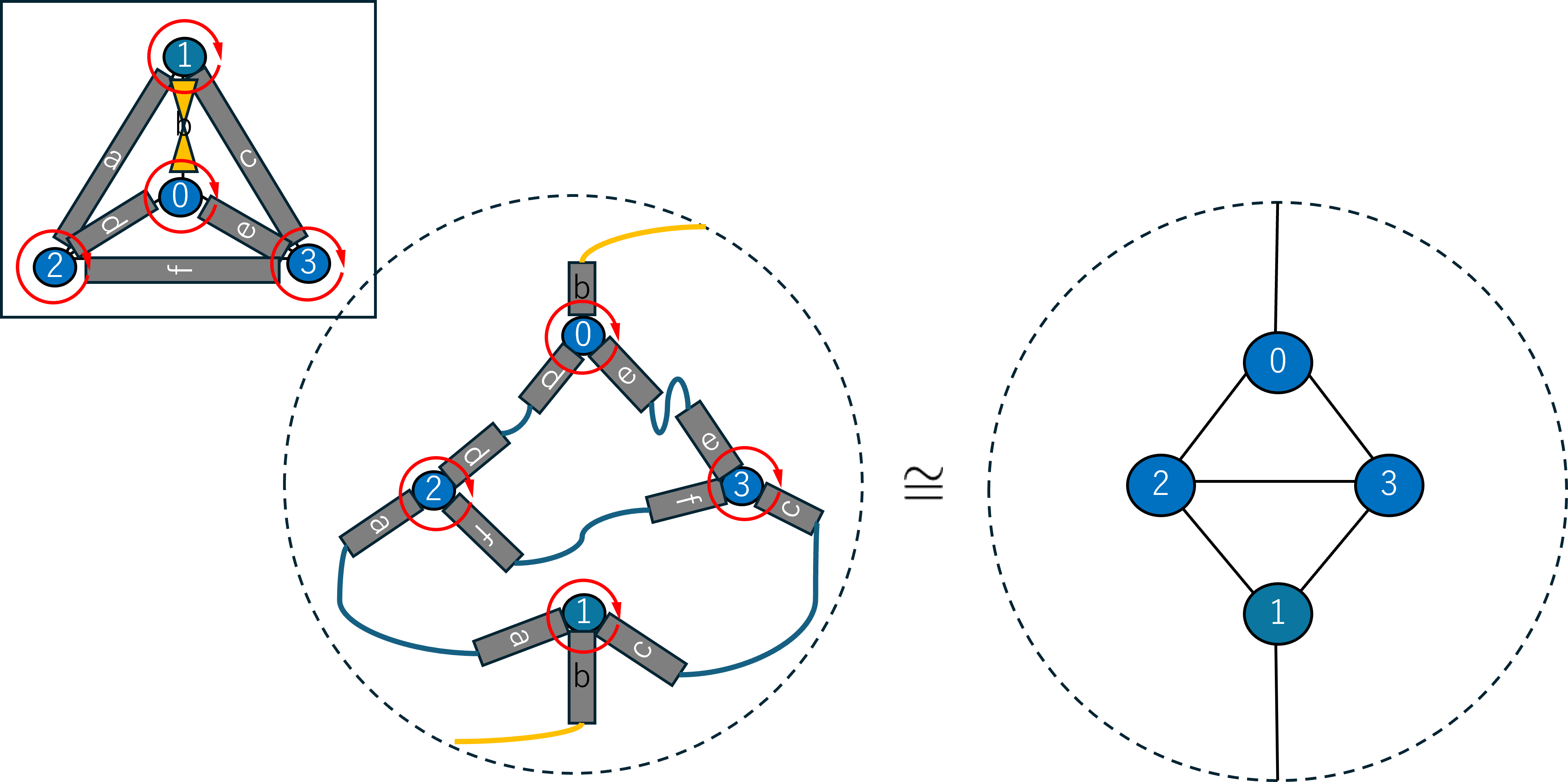
The blow up graph of $G=(V,A)$ with the rotation $\rho$ is obtained by replacing each vertex of $G$ into the directed cycle following the rotation assigned to each vertex and conserving the adjacency relation of the original graph as follows. The vertex set of the blow up graph $G^{BU}(\rho)=(X^{BU}(\rho),A^{BU}(\rho))$ is denoted by

X^{BU}(\rho)=A;

the arc set of the blow up graph is denoted by the disjoint union of

A^{BU}(\rho)=A_{br}\sqcup A_{is},

which are called the bridge and the island, respectively. Here the “bridge” $A_{br}$ and the “island” $A_{is}$ are both isomorphic to $A$ and denoted by

A_{is}=\{(e,\rho(e))\;|\;e\in A\},\;A_{br}=\{(e,\bar{e})\;|\;e\in A\}.

See Figure 8 (c).

Let us give some remarks and introduce some new notations which will be important to describe the time evolution of our quantum walk model.

Remark 4.1.

It holds that for $e\in A$ with $t(e)=x\in X$ in $G$ ,

\{(e^{\prime},\;\rho(e^{\prime}))\;|\;\text{$t(e^{\prime})=x$ in $G$}\}=\{(\;\rho^{j}(e),\;\rho^{j+1}(e)\;)\;|\;j=0,1,\dots,\deg_{G}(x)-1\}\subset A_{is}.

We call the above directed cycle induced by $x\in X$ the island of $x\in X$ which is denoted by $A_{is}(x)$ . On the other hand, for $\epsilon\in E$ with the end vertices $x,y\in X$ in $G$ , $(e,\bar{e})$ and $(\bar{e},e)$ , where $|e|=\epsilon$ , are called the bridge between the islands $x$ and $y$ . Then let us define

\rho(\boldsymbol{e}_{is}):=(\rho(e),\rho^{2}(e))

for an island arc $\boldsymbol{e}_{is}=(e,\rho(e))$ , and

\bar{\boldsymbol{e}}_{br}:=(\bar{e},e),\;\tau(\boldsymbol{e}_{br})=\tau(|e|)

for a bridge arc $\boldsymbol{e}_{br}=(e,\bar{e})$ .

Remark 4.2.

The in-degree and out-degree for every vertex of the blow-up graph are equally $2$ .

For each vertex $e\in X^{BU}$ , the incoming arcs to $e$ come from the vertex $\rho^{-1}(e)$ along the island of $t_{G}(e)$ and the vertex $\bar{e}$ along the bridge between the islands $t(e)$ and $o(e)$ while the outgoing arcs to $e$ go out to the vertex $\rho(e)$ along the island of $t_{G}(e)$ and the vertex $\bar{e}$ along the bridge between the islands $t(e)$ and $o(e)$ .

Then for any island arc $\boldsymbol{e}_{is}\in A_{is}$ , there are exactly two bridge arcs $\boldsymbol{e}_{br}$ and $\boldsymbol{e}_{br}^{\prime}\in A_{br}$ such that $o(\boldsymbol{e}_{is})=t(\boldsymbol{e}_{br})$ and $t(\boldsymbol{e}_{is})=t(\boldsymbol{e}_{br}^{\prime})$ , respectively. Such bridge arcs for the island arc $\boldsymbol{e}_{is}$ are denoted by

\boldsymbol{e}_{br}:=\mathrm{br}(\boldsymbol{e}_{is}),\;\boldsymbol{e}_{br}^{\prime}:=\mathrm{br}^{\sharp}(\boldsymbol{e}_{is}),

respectively. On the other hand, for any bridge arc $\boldsymbol{e}_{br}\in A_{br}$ , there is exactly two island arcs $\boldsymbol{e}_{is}$ and $\boldsymbol{e}_{is}^{\prime}$ such that $o(\boldsymbol{e}_{br})=t(\boldsymbol{e}_{is})=o(\boldsymbol{e}_{is}^{\prime})$ . Such island arcs for the bridge arc $\boldsymbol{e}_{br}$ are denoted by

\boldsymbol{e}_{is}:=\mathrm{is}(\boldsymbol{e}_{br}),\;\boldsymbol{e}_{is}^{\prime}:=\mathrm{is}^{\sharp}(\boldsymbol{e}_{br}),

respectively.

4.3 Quantum walk on the rotation system $(G,\rho,\tau)$

For given the rotation system $(G,\rho,\tau)$ , let us consider the blow up graph of $G^{\tau}$ induced by the rotation $\rho\oplus\rho^{-1}$ by replacing $G$ discussed in the previous subsection 4.2 with $G^{\tau}$ discussed also in subsection 4.1. This blow up graph is denoted by $G(\rho,\tau)=(X(\rho,\tau),A(\rho,\tau))$ . Note that $G(\rho,\tau)={G^{\tau}}^{BU}(\rho\oplus\rho^{-1})$ .

Now we are ready to describe the dynamics of this quantum walk model. The total state space of our quantum walk is given by the vector space

\mathcal{H}_{total}=\mathbb{C}^{A(\rho,\tau)}.

In our quantum walk model, a local time evolution at each vertex of $G(\rho,\tau)$ is represented by a $2$ -dimensional unitary matrix, because the degree of the blow up graph is $2$ , and if a quantum walk passes through the twisted bridge, the phase of the quantum walker is converted by $e^{i\pi}=-1$ .

In the following, we represent this dynamics of our quantum walk model in more precisely. Let $W:\mathbb{C}^{A(\rho,\tau)}\to\mathbb{C}^{A(\rho,\tau)}$ be the unitary time evolution operator such that for each time step $t\in\mathbb{N}$ , the total state of the quantum walk at time $t$ , $\psi_{t}\in\mathbb{C}^{A(\rho,\tau)}$ , is given by

\psi_{t+1}=W\psi_{t}\text{ for $t\geq 0$}

with some initial state $\psi_{0}\in\mathbb{C}^{A(\rho,\tau)}$ . The unitary time evolution operator $W$ is defined as follows.

Definition 4.1.

Let us set a $2\times 2$ unitary matrix by

C=\begin{bmatrix}a&b\\ c&d\end{bmatrix}.

For any island arc $\boldsymbol{e}_{is}\in A_{is}\subset A(\rho,\tau)$ , bridge arc $\boldsymbol{e}_{br}\in A_{br}\subset A(\rho,\tau)$ , the time evolution operator $W$ is defined by

	$\displaystyle(W\psi)(\boldsymbol{e}_{is})$	$\displaystyle=a\;\psi(\rho^{-1}(\boldsymbol{e}_{is}))+b\;\psi(\mathrm{br}(\boldsymbol{e}_{is}))$		(4.13)
	$\displaystyle(W\psi)(\boldsymbol{e}_{br})$	$\displaystyle=(-1)^{\tau(\boldsymbol{e}_{br})}\left\{c\;\psi(\mathrm{is}(\boldsymbol{e}_{br}))+d\;\psi(\bar{\boldsymbol{e}}_{br})\right\}$		(4.14)

for any $\psi\in\mathbb{C}^{A(\rho,\tau)}$ .

Remark 4.3.

For any bridge arc $\boldsymbol{e}_{br}\in A_{br}\subset A(\rho,\tau)$ , the local time evolution on the vertex $o(\boldsymbol{e}_{br})\in X(\rho,\tau)$ is described by

\begin{bmatrix}\psi_{t+1}(\;\mathrm{is}^{\sharp}(\boldsymbol{e}_{br})\;)\\ \psi_{t+1}(\boldsymbol{e}_{br})\end{bmatrix}=\begin{bmatrix}1&0\\ 0&(-1)^{\tau(\boldsymbol{e}_{br})}\end{bmatrix}\;C\begin{bmatrix}\psi_{t}(\;\mathrm{is}(\boldsymbol{e}_{br})\;)\\ \psi_{t}(\bar{\boldsymbol{e}}_{br})\end{bmatrix}.

(4.15)

4.4 Extension to an infinite system

For the blow-up graph $G(\rho,\tau)$ , let us choose a subset of $A_{is}$ by $\delta A_{is}$ as the boundary to the “outside”. We deform this blow-up graph to an infinite graph by the following procedure.

(1)

Every $e\in A(\rho,\tau)\setminus\delta A_{is}$ is left as it is without any transformations.
(2)

Each $e\in\delta A_{is}$ is divided by two arcs by replacing $e$ with two new arcs $\xi_{out}$ and $\xi_{in}$ satisfying with $o(e)=o(\xi_{out})$ , $t(\xi_{out})=o(\xi_{in})$ and $t(\xi_{in})=t(e)$ .
(3)

Semi-infinite path $\mathbb{P}_{e}$ with the root vertex $o(\mathbb{P}_{e})$ is joined by identifying $o(\mathbb{P}_{e})$ with $t(\xi_{out})=o(\xi_{in})$ . The pair of $(\xi_{out},\xi_{in})$ is called the quay of $e\in\delta A_{is}$ . The sets of such as $\xi_{out}$ and $\xi_{in}$ are denoted by $\delta A_{qy}^{-}$ and $\delta A_{qy}^{+}$ , respectively.

The resulting graph is denoted by ${\tilde{G}}(\rho,\tau)=(\tilde{X}(\rho,\tau),\tilde{A}(\rho,\tau))$ , which is an infinite graph. See Figure 8 (d). The set of boundary vertices of $\tilde{G}(\rho,\tau)$ is defined by

\delta X=\bigcup_{e\in\delta A_{is}}o(\mathbb{P}_{e})\subset{\tilde{X}}(\rho,\tau).

The set of arcs of tails is denoted by $A_{tl}$ . The subset of $A_{tl}$ called the pier is denoted by

\delta A_{pr}^{+}=\{e\in A_{tl}\;|\;t(e)\in\delta X\},\;\delta A_{pr}^{-}=\{e\in A_{tl}\;|\;o(e)\in\delta X\}.

Note that for each island having a boundary vertex, the local rotation in $\tilde{G}(\rho,\tau)$ is “expanded” by the insertion of the tail. Let us use the same notation for the new rotation as $\rho$ to reduce the number of notations. Let $\tilde{A}_{is}\subset{\tilde{A}}^{BU}$ be the set of the islands of $\tilde{G}(\rho,\tau)$ following the rotation $\rho$ . Let $\tilde{A}_{br}$ be the union of $A_{br}$ and $\delta A_{pr}$ . The designation of the twist to $A_{tl}$ is assigned by $0$ .

The total state space here is extended to

\tilde{\mathcal{H}}_{total}=\mathbb{C}^{\tilde{A}(\rho,\tau)}.

The time evolution operator $\tilde{W}$ on $\mathbb{C}^{\tilde{A}(\rho,\tau)}$ is given as follows, which is essentially the same as Definition 4.1 except the boundaries and the tails but the setting of the initial state is crucial to obtain the stationary state:

Definition 4.2.

Let $\Psi_{t}$ be the $t$ -th iteration of $\tilde{W}$ , such that $\Psi_{t}=\tilde{W}\Psi_{t-1}$ $t=1,2,\dots$ with the initial state $\Psi_{0}$ defined in (4.17).

The time evolution $\tilde{W}$ .

(1)

For $\boldsymbol{e}\in A_{tl}\setminus\delta A_{pr}^{-}$ : The arcs of a tail is put by $e_{0},e_{1},\dots$ and $\bar{e}_{0},\bar{e}_{1},\dots$ with $t(e_{0})\in\delta X$ $t(e_{j+1})=o(e_{j})$ $j=0,1,2,\dots$ . The time evolution on the tail is free, that is,

$\Psi_{t+1}(e_{j})=\Psi_{t}(e_{j+1}),\;\Psi_{t+1}(\bar{e}_{j+1})=\Psi_{t}(\bar{e}_{j})$ (4.16)

for any $j=0,1,2,\dots$ .

(2)

For $\boldsymbol{e}\in\tilde{A}_{is}\cup A_{br}\cup\delta A_{pr}^{-}$ : For any island arc $\boldsymbol{e}_{is}\in\tilde{A}_{is}$ , “bridge or pier” arc $\boldsymbol{e}_{br}\in A_{br}\cup\delta A_{pr}^{-}$ ,

	$\displaystyle\Psi_{t+1}(\boldsymbol{e}_{is})$	$\displaystyle=a\;\Psi_{t}(\rho^{-1}(\boldsymbol{e}_{is}))+b\;\Psi_{t}(\mathrm{br}(\boldsymbol{e}_{is})),$
	$\displaystyle\Psi_{t+1}(\boldsymbol{e}_{br})$	$\displaystyle=(-1)^{\tau(\boldsymbol{e}_{br})}\left\{c\;\Psi_{t}(\mathrm{is}(\boldsymbol{e}_{br}))+d\;\Psi_{t}(\bar{\boldsymbol{e}}_{br})\right\}.$

Here if $\boldsymbol{e}_{is}\in\delta A_{qy}^{\pm}$ , the bridge arc $\mathrm{br}(\boldsymbol{e}_{is})\in\delta A_{pr}^{-}$ is the pier from $t(\boldsymbol{e}_{is})$ ; if $\boldsymbol{e}_{br}\in\delta A_{pr}^{-}$ , the island arc $\mathrm{is}(\boldsymbol{e}_{br})\in\delta A_{qy}^{-}$ is the quay of the boundary vertex $o(\boldsymbol{e}_{br})$ .

The initial state $\Psi_{0}$ .
Let each tail is labeled by each element of $\delta A_{pr}^{+}$ . Prepare the sequence of complex values $(\alpha_{e})_{e\in\delta A_{pr}^{+}}$ . Then we set the following uniformly bounded initial state on the tails:

\Psi_{0}(e^{\prime})=\begin{cases}\alpha_{e}&\text{: $e^{\prime}\in A(\mathbb{P}_{e})$, ${\rm dist}(t(e^{\prime}),o(\mathbb{P}_{e}))>{\rm dist}(t(e^{\prime}),o(\mathbb{P}_{e}))$ ($e\in\delta A_{is}$),}\\ 0&\text{ otherwise.}\end{cases}

(4.17)

Note that the initial state $\Psi_{0}$ is bounded but no longer square summable. Such a setting of initial state provides a constant inflow from the tails at very time step. On the other hand, the setting of the time evolution on tails implies an outflow from the interior. Under this setting, the convergence to a fixed point of this quantum walk is ensured in the following meaning:

Proposition 4.2 ([8]).

For any $e\in\tilde{A}(\rho,\tau)$ ,

\exists\lim_{t\to\infty}\Psi_{t}(e)=\Psi_{\infty}(e).

5 Unitary equivalence

Let $(G,\rho,\tau)$ be a rotation system whose underlying abstract graph is $G=(X,A)$ . Let us deform the rotation system as follows which is corresponding to Operation iii.

Operation ( $\star$ )
Choose a one vertex from $G$ , say $x\in X$ . Then let us reverse its rotation and switch all the edge types of the incident edges of $x$ . Such a rotation system is denoted by $(G,\rho^{(x)},\tau^{(x)})$ .

By Lemma 4.1, the resulting embeddings on a closed surface of the rotation systems of the double covering graph, $(G^{\tau},\rho\oplus\rho^{-1},\mathrm{id})$ and $(G^{\tau^{(x)}},\rho^{(x)}\oplus{\rho^{(x)}}^{-1},\mathrm{id})$ , are isomorphic to each other. Under these isomorphic two embeddings, we take the blow up and choose the boundary island arcs $\delta A$ from $G(\rho,\tau)$ and its isomorphic boundary $\delta A^{\prime}$ from $G(\rho^{(x)},\tau^{(x)})$ . The resulting blow up graphs are denoted by $\tilde{G}(\rho,\tau)$ and $\tilde{G}(\rho^{(x)},\tau^{(x)})$ , respectively. Note that they are still isomorphic to each other: $\tilde{G}(\rho,\tau)\cong\tilde{G}(\rho^{(x)},\tau^{(x)})$ under the following bijection $\phi$ for the incident arcs of islands $x$ and $x^{\prime}$ :

Bijection $\phi:\tilde{G}(\rho,\tau)\to\tilde{G}(\rho^{\prime},\tau^{\prime})$ satisfies the following:

(1)

island :
$e_{is}=(e,\tilde{\rho}(e))\in A_{is}(x,k)\subset A(\rho,\tau)$
with $o(e)=(y,k^{\prime})$ and $o(\tilde{\rho}(e))=(z,k^{\prime\prime})$ in $G^{\tau}$
$\leftrightarrow$
$\phi(e_{is})=(e^{\prime},\tilde{\rho}(e^{\prime}))\in A_{is}(x,k+1)\subset A(\rho,\tau)$
with $o(e^{\prime})=(z,k^{\prime\prime}+1)$ and $t(\tilde{\rho}(e^{\prime}))=(y,k^{\prime}+1)$ in $G^{\tau}$ .
(2)

bridge :
$e\in A_{br}\subset A(\rho,\tau)$
with $o(e)=(x,\ell)$ and $t(e)=(y,m)$ in $G^{\tau}$
$\leftrightarrow$
$\phi(e)\in A^{\prime}_{br}\subset A(\rho^{\prime},\tau^{\prime})$
with $o(e)=(x,\ell+1)$ and $t(e)=(y,m+1)$ in $G^{\tau}$

The other arcs are left nothing as it is.

In this section, we show that the time evolution operators $\tilde{W}$ on $\tilde{G}(\rho,\tau)$ and $\tilde{W}^{(x)}$ on $\tilde{G}(\rho^{(x)},\tau^{(x)})$ are unitarily equivalent. Indeed we have the following proposition.

Proposition 5.1.

Let the rotation system $(G,\rho,\tau)$ and $(G,\rho^{\prime},\tau^{\prime})$ are isomorphic to each other, and let the boundaries of the induced blow-up graphs are also isomorphic to each other. Then the time evolution operators $W$ on $\tilde{G}(\rho,\tau)$ and $W^{\prime}$ on $\tilde{G}(\rho^{\prime},\tau^{\prime})$ are unitarily equivalent, that is, there is an unitary map $\mathcal{U}$ such that

W^{\prime}=\mathcal{U}^{*}\;W\;\mathcal{U}.

Proof.

It is sufficient to consider the case for $\rho^{\prime}=\rho^{x}$ for arbitrary $x\in X$ . By Lemma 4.1, “the reversing the rotation of $x$ ” and “the reversing all the incident edges of $x$ ” are reflected in the corresponding time evolution operator on $\tilde{G}(\rho,\tau)$ :

(1)

Switching the labels of all the arcs associated to $(x,0)$ and $(x,1)$ following the bijection $\phi$ ( $\leftrightarrow$ Reversing the rotation of $x$ );

(2)

Changing the twist $\tau$ to $\tau^{\prime}$ by

\tau^{\prime}(e)=\begin{cases}\tau(e)+1&\text{: $e$ is incident to $(x,0)$ or $(x,1)$ in $G^{\tau}$,}\\ \tau(e)&\text{: otherwise.}\end{cases}

( $\leftrightarrow$ Reversing all the incident edges of $x$ )

Obviously, the operation (1) has the corresponding unitary map. This map is denoted by $\mathcal{U}_{\phi}$ , that is,

(\mathcal{U}_{\phi}\psi)(e)=\psi(\phi^{-1}(e)).

Then in the rest of the discussion, let us find the corresponding unitary map of the operation (2). To this end, for the blow-up graph $\tilde{G}(\rho,\tau)$ , set

\mathcal{A}:=\{\theta:A(\rho,\tau)\to\mathbb{C}\;|\;\theta(e)=0\text{ for all $e\in A_{is}$},\;\theta(\bar{e})=-\theta(e)\text{ for all $e\in A_{br}$}\}.

Note that if we set

\theta(e)=\begin{cases}\pi&\text{: $e\in A_{br}$ with $\tau(e)=1$}\\ 0&\text{: otherwise}\end{cases}

(5.18)

then $\tau(e)=e^{\boldsymbol{\rm i}\;\theta(e)}$ for any $e\in A_{br}$ , where $\boldsymbol{\rm i}=\sqrt{-1}$ . On the other hand if we set

\theta(e)=\begin{cases}\pi&\text{: $e\in A_{br}$ with $\tau^{\prime}(e)=1$}\\ 0&\text{: otherwise}\end{cases}

(5.19)

then $\tau^{\prime}(e)=e^{\boldsymbol{\rm i}\;\theta(e)}$ for any $e\in A_{br}$ . For $\theta\in\mathcal{A}$ , and arbitrary path in $G(\rho,\tau)$ , $p=(a_{1},a_{2},\dots,a_{k})$ with $t(a_{j})=o(a_{j+1})$ $(j=1,\dots,k-1)$ , we define

\int_{p}\theta:=\sum_{j=1}^{k}\theta(e_{j}).

A path $p=(a_{1},\dots,a_{r})$ with $a_{1}\in A_{br}$ , $a_{r}\in A_{is}$ in $G(\rho,\tau)$ may be represented by

p=(\;e_{1},\xi_{1},\tilde{\rho}^{1}(\xi_{1}),\dots,\tilde{\rho}^{k_{1}}(\xi_{1}),\;e_{2},\;\xi_{2},\tilde{\rho}^{1}(\xi_{2}),\dots,\tilde{\rho}^{k_{2}}(\xi_{2}),\;e_{3},\;\xi_{3},\tilde{\rho}^{1}(\xi_{3}),\dots,\tilde{\rho}^{k_{3}}(\xi_{3}),\dots{\\ }\dots,e_{r},\xi_{r},\tilde{\rho}^{1}(\xi_{r}),\dots,\tilde{\rho}^{k_{r}}(\xi_{r})\;),

where $\xi_{j},\tilde{\rho}^{s}(\xi_{j})\in A_{is}$ and $e_{j}\in A_{br}$ . Here if there is a back-tracking in $p$ , a corresponding subsequence of a walk on an island disappears. The inverse path of $p$ is defined by

\bar{p}=(\;\tilde{\rho}^{k_{r}+1}(\xi_{r}),\tilde{\rho}^{k_{r}+2}(\xi_{r}),\dots,\tilde{\rho}^{d_{r}-1}(\xi_{r}),\;\bar{e}_{r},\dots{\\ }\dots,\tilde{\rho}^{k_{3}+1}(\xi_{3}),\tilde{\rho}^{k_{3}+2}(\xi_{3}),\dots,\tilde{\rho}^{d_{3}-1}(\xi_{3}),\;\bar{e}_{2},\tilde{\rho}^{k_{1}+1}(\xi_{1}),\tilde{\rho}^{k_{1}+2}(\xi_{1}),\dots,\tilde{\rho}^{d_{1}-1}(\xi_{1}),\;\bar{e}_{1}\;),

where $\tilde{\rho}:=\rho\oplus\rho^{-1}$ . The inverse path of $p$ for the other cases and $p$ with back-trackings case are also defined in the same way.

Lemma 5.1.

Set $\theta_{1},\theta_{2}\in\mathcal{A}$ . If $\int_{c}\theta_{1}=\int_{c}\theta_{2}$ for any close path $c$ in $G(\rho,\tau)$ , then $\int_{p}(\theta_{2}-\theta_{1})=\int_{p^{\prime}}(\theta_{2}-\theta_{1})$ for any path $p$ and $p^{\prime}$ with $o(p)=o(p^{\prime})$ and $t(p)=t(p^{\prime})$ .

Proof.

It holds that $\int_{\bar{p}}\theta=-\int_{p}\theta$ for any path $p$ by the definition. Note that $p\cup\bar{p^{\prime}}$ is a closed cycle. Then we have

0=\int_{p\cup\bar{p}}(\theta_{2}-\theta_{1})=\int_{p}(\theta_{2}-\theta_{1})+\int_{\bar{p^{\prime}}}(\theta_{2}-\theta_{1})=\int_{p}(\theta_{2}-\theta_{1})-\int_{p^{\prime}}(\theta_{2}-\theta_{1}),

which is the conclusion. ∎

Lemma 5.1 tells us that the value $\int_{p}(\theta_{2}-\theta_{1})$ is independent of routes from $o(p)$ to $t(p)$ . Let us fix a vertex $x_{*}$ . Since $\int_{p}(\theta_{2}-\theta_{1})$ for a path starting from $x_{*}$ is determined by $t(p)=x$ , we set such a value by $\Delta(x)$ , which is well-defined.

Let $\psi_{t}$ (resp. $\psi_{t}^{\prime}$ ) be the $t$ -th iteration of $\tilde{W}$ (resp. $\tilde{W^{\prime}}$ ) with the twist $\tau$ (resp. $\tau^{\prime}$ ) such that $\psi_{t+1}=\tilde{W}\psi_{t}$ (resp. $\psi^{\prime}_{t+1}=\tilde{W}^{\prime}\psi_{t}^{\prime}$ ). By Remark 4.3, we have

\begin{bmatrix}\psi_{t+1}(\xi)\\ \psi_{t+1}(\epsilon)\end{bmatrix}=\begin{bmatrix}e^{\boldsymbol{\rm i}\;\theta_{1}(\xi)}&0\\ 0&e^{\boldsymbol{\rm i}\;\theta_{1}(\epsilon)}\end{bmatrix}\;C\begin{bmatrix}\psi_{t}(\xi^{\flat})\\ \psi_{t}(\bar{\epsilon})\end{bmatrix},

(5.20)

for any $\epsilon\in A_{br}$ , where $\xi^{\flat}=\mathrm{is}(\epsilon)$ and $\xi=\mathrm{is}^{\sharp}(\epsilon)$ . Here $\theta_{1}$ is defined in (5.18). Now let us set $\theta_{2}$ by (5.19). The operation $(\star)$ keeps the parity of any cycles passing through the vertex $x$ , because $\tau(e)+\tau(e^{\prime})$ with $t(e)=x=o(e)$ in $G$ is changed to

\tau^{\prime}(e)+\tau^{\prime}(e^{\prime})=\tau(e)+1+\tau(e^{\prime})+1=\tau(e)+\tau(e^{\prime}),

which implies $\int_{c}\theta_{1}=\int_{c}\theta_{2}$ for any cycle $c$ in $\tilde{G}$ . Let us consider a path $p$ with $o(p)=x_{*}$ and $t(p)=o(\xi)=o(\epsilon)$ in $\tilde{G}$ . Thus we have

	$\displaystyle\Delta(t(\xi))$	$\displaystyle=\int_{p+\xi}(\theta_{2}-\theta_{1})=\int_{p}(\theta_{2}-\theta_{1})+\theta_{2}(\xi)-\theta_{1}(\xi)$
		$\displaystyle=\Delta(o(\xi))+\theta_{2}(\xi)-\theta_{1}(\xi),$
	$\displaystyle\Delta(t(e))$	$\displaystyle=\int_{p+e}(\theta_{2}-\theta_{1})=\int_{p}(\theta_{2}-\theta_{1})+\theta_{2}(e)-\theta_{1}(e)$
		$\displaystyle=\Delta(o(\epsilon))+\theta_{2}(e)-\theta_{1}(e),$

Here $\Delta(x)$ with a fixed vertex $x_{*}\in\tilde{X}$ is well-defined by Lemma 5.1. Inserting them into (5.20), we have

	$\displaystyle\begin{bmatrix}e^{\boldsymbol{\rm i}\;\Delta(\;t(\xi)\;)}\;\psi_{t+1}(\xi)\\ e^{\boldsymbol{\rm i}\;\Delta(\;t(\epsilon)\;)}\;\psi_{t+1}(\epsilon)\end{bmatrix}$	$\displaystyle=\begin{bmatrix}e^{\boldsymbol{\rm i}\;\theta_{2}(\xi)}&0\\ 0&e^{\boldsymbol{\rm i}\;\theta_{2}(\epsilon)}\end{bmatrix}\begin{bmatrix}e^{\boldsymbol{\rm i}\;\Delta(\;o(\xi)\;)}&0\\ 0&e^{\boldsymbol{\rm i}\;\Delta(\;o(\epsilon)\;)}\end{bmatrix}\;C\;\begin{bmatrix}\psi_{t}(\xi^{\flat})\\ \psi_{t}(\bar{\epsilon})\end{bmatrix}$
		$\displaystyle=\begin{bmatrix}e^{\boldsymbol{\rm i}\;\theta_{2}(\xi)}&0\\ 0&e^{\boldsymbol{\rm i}\;\theta_{2}(\epsilon)}\end{bmatrix}\;C\;\begin{bmatrix}e^{\boldsymbol{\rm i}\;\Delta(\;t(\xi^{\flat})\;)}\;\psi_{t}(\xi^{\flat})\\ e^{\boldsymbol{\rm i}\;\Delta(\;t(\bar{\epsilon})\;)}\;\psi_{t}(\bar{\epsilon})\end{bmatrix}$

The second equality derives from $o(\xi)=o(\epsilon))$ which gives the commutativity of the second diagonal matrix and $C$ in first equality. Therefore introducing the unitary map $\mathcal{U}_{\Delta}$ by

(\mathcal{U}_{\Delta}\psi)(a)=e^{\boldsymbol{\rm i}\;\Delta(t(a))}\;\psi(a),

we obtain

W^{\prime}=(\mathcal{U}_{\Delta}\mathcal{U}_{\phi})^{*}\;W\;(\mathcal{U}_{\Delta}\mathcal{U}_{\phi}).

∎

Remark 5.1.

For a vertex $(x,j)\in X(\rho,\tau)$ , define $\mathrm{sheet}(x,j):=j\in\mathbb{Z}_{2}$ . Then the unitary map $\mathcal{U}=\mathcal{U}_{\Delta}\;\mathcal{U}_{\phi}$ is described by

(\mathcal{U}\psi)(a)=\begin{cases}\psi(\phi^{-1}(a))&\text{: $\mathrm{sheet}(t(a))+\mathrm{sheet}(x_{*})=\mathrm{sheet}(\phi(t(a)))+\mathrm{sheet}(\phi(x_{*}))$,}\\ -\psi(\phi^{-1}(a))&\text{: $\mathrm{sheet}(t(a))+\mathrm{sheet}(x_{*})\neq\mathrm{sheet}(\phi(t(a)))+\mathrm{sheet}(\phi(x_{*}))$.}\end{cases}

6 Scattering

6.1 The scattering matrix represented by faces

For the blow-up graph $G(\rho,\tau)$ , let $\delta X=\{x_{1},\dots,x_{\kappa}\}$ and $\delta A_{pr}^{+}=\{e_{1},\dots,e_{\kappa}\}$ such that $t(e_{j})=x_{j}$ . The stationary state is denoted by $\Psi_{\infty}\in\mathbb{C}^{\tilde{A}(\rho,\tau)}$ . Let us represent the inflow from the outside by $\boldsymbol{\alpha}_{in}\in\mathbb{C}^{\delta X}$ such that

\boldsymbol{\alpha}_{in}(x)=\Psi_{\infty}(e)\text{ with $t(e)=x$}

for any $x\in\delta X$ , $\ell\in\mathbb{Z}_{2}$ , while the outflow to the outside by $\boldsymbol{\beta}_{out}\in\mathbb{C}^{\delta X}$ such that

\boldsymbol{\beta}_{out}(x)=\Psi_{\infty}(\bar{e})\text{ with $t(e)=x$}

for any $x\in\delta X$ . The scattering matrix $S:\mathbb{C}^{\delta X}\to\mathbb{C}^{\delta X}$ is defined by

\boldsymbol{\beta}_{out}=S\boldsymbol{\alpha}_{in},

which is determined by the rotation system $G(\rho,\tau)$ and $\delta X$ , and independent of $\boldsymbol{\alpha}_{in}$ , $\boldsymbol{\beta}_{out}$ . It is shown in [8] that such a matrix $S$ exists and is unitary. However its explicit expression is up to the individual setting.

We prepare important graph notions which express the scattering matrix. Let $f=(e_{0},\dots,e_{\kappa-1})\in F$ be a facial closed walk of the rotation system $(G^{\tau},\rho\oplus\rho^{-1},\mathrm{id})$ with length $\kappa=|f|$ . The extended facial walk of $\tilde{f}$ in $A(\rho,\tau)$ is defined by just alternatively inserted corresponding island arcs into each arc of $f$ ; (we use the same notation for the extended facial walk by $f$ ):

f:=(\;\xi_{0},e_{0},\dots,\xi_{\kappa-1},e_{\kappa-1}\;),

(6.21)

where $e_{j}\in A_{br}\cong A$ and $\xi_{j}\in A_{is}$ with

\xi_{j}=\mathrm{is}(e_{j}),\;e_{j}=\mathrm{br}(\xi_{j+1})

(6.22)

for any $j\in\{0,1,\dots,\kappa-1\}$ in the modulus of $\kappa$ . Here if $\xi_{j}\in\delta A_{is}$ , $\xi_{j}$ represents the quay arcs $(\xi_{j}^{+},\xi_{j}^{-})$ . Let $\delta F\subset F$ be the set of (extended) facial walk passing through a boundary vertex $\delta X$ in $\tilde{G}$ . For any facial walk $f$ , there exists a chiral facial walk $f^{*}$ defined by going around the opposite direction on the opposite sheet. We introduce the following useful lemma to consider the scattering.

Lemma 6.1.

Assume $d\in\mathbb{R}$ . Let $\psi_{\infty}\in\mathcal{H}$ be the stationary state. Set $\omega=-\det(C)$ . For each facial walk $f\in\delta F$ of the orientation system $(G,\rho,\tau)$ represented by a sequence of $\Omega$ ,

f:=(\;\xi_{0},e_{0},\xi_{1},e_{1},\dots,\xi_{\kappa-1},e_{\kappa-1}\;),

we have

\psi_{\infty}(\xi^{\prime}_{j+1})=(-1)^{\tau(e_{j})}\omega\;\psi_{\infty}(\xi_{j}^{\prime\prime}),\;(j=0,1,\dots,\kappa-1)

where if $\xi_{j+1}\in\delta A_{is}$ , then $\xi_{j+1}^{\prime}=\xi_{j+1}^{+}$ , otherwise $\xi_{j+1}$ ; if $\xi_{j}\in\delta A_{is}$ , then $\xi_{j}^{\prime\prime}=\xi_{j}^{-}$ , otherwise $\xi_{j}^{\prime\prime}=\xi_{j}$ .

Proof.

For any bridge arcs $e\in A_{br}$ , (of course) the vertices $o(e)$ and $t(e)$ are connected by the bridge arcs $e^{R}_{1}:=e$ and $e^{L}_{1}:=\bar{e}$ , moreover the island arcs $e_{0}^{R}:=\mathrm{is}(e)$ and $e_{0}^{L}:=\mathrm{is}^{\sharp}(e)$ are connected to $o(e)$ , while the island arcs $e_{2}^{R}:=\mathrm{is}^{\sharp}(\bar{e})$ and $e_{2}^{L}:=\mathrm{is}(\bar{e})$ are connected to $o(t)$ . Then the blow up graph has locally a path structure with $2$ vertices and “ $6$ ” symmetric arcs. Let us see this fact leads a transfer matrix discussed in the spectral analysis on the discrete-time quantum walks on the one-dimensional lattice and gives the conclusion. Let us set $\psi:=\psi_{\infty}$ . The point to get the transfer matrix is to align the “subscriptions” for each vector: the local eigenequation is rewritten by

\displaystyle\begin{bmatrix}-a&1\\ -c^{\prime}&0\end{bmatrix}\begin{bmatrix}\psi(e_{0}^{R})\\ \psi(e_{0}^{L})\end{bmatrix}=\begin{bmatrix}0&b\\ -1&d^{\prime}\end{bmatrix}\begin{bmatrix}\psi(e_{1}^{R})\\ \psi(e_{1}^{L})\end{bmatrix}\text{ and }\begin{bmatrix}1&-a\\ 0&-c^{\prime}\end{bmatrix}\begin{bmatrix}\psi(e_{2}^{R})\\ \psi(e_{2}^{L})\end{bmatrix}=\begin{bmatrix}b&0\\ d^{\prime}&-1\end{bmatrix}\begin{bmatrix}\psi(e_{1}^{R})\\ \psi(e_{1}^{L})\end{bmatrix}

(6.23)

where $c^{\prime}=(-1)^{\tau(e)}c$ , $d^{\prime}=(-1)^{\tau(e)}d$ . Therefore we have

	$\displaystyle\begin{bmatrix}\psi(e_{2}^{R})\\ \psi(e_{2}^{L})\end{bmatrix}$	$\displaystyle=\begin{bmatrix}1&-a\\ 0&-c^{\prime}\end{bmatrix}^{-1}\begin{bmatrix}b&0\\ d^{\prime}&-1\end{bmatrix}\begin{bmatrix}0&b\\ -1&d^{\prime}\end{bmatrix}^{-1}\begin{bmatrix}-a&1\\ -c^{\prime}&0\end{bmatrix}\begin{bmatrix}\psi(e_{0}^{R})\\ \psi(e_{0}^{L})\end{bmatrix}$
		$\displaystyle=\frac{1}{\|c\|^{2}\omega^{\prime}}\begin{bmatrix}\omega^{\prime}&0\\ 0&1\end{bmatrix}\begin{bmatrix}1-{\bar{d^{\prime}}}^{2}&d^{\prime}-\bar{d^{\prime}}\\ -d^{\prime}+\bar{d^{\prime}}&1-{d^{\prime}}^{2}\end{bmatrix}\begin{bmatrix}\omega^{\prime}&0\\ 0&1\end{bmatrix}\begin{bmatrix}\psi(e_{0}^{R})\\ \psi(e_{0}^{L})\end{bmatrix}$

where $\omega^{\prime}=(-1)^{\tau(e)}\omega$ . Here the second equality is obtained by the properties of the unitarity matrix $C$ , for examples, $a=-\omega^{\prime}\bar{d^{\prime}}$ , $b=\omega^{\prime}\bar{c^{\prime}}$ , $|d^{\prime}|^{2}+|c^{\prime}|^{2}=1$ . Then $d\in\mathbb{R}$ if and only if $\psi(e_{2}^{R})=\omega^{\prime}\psi(e_{0}^{R})$ and $\psi(e_{0}^{L})=\omega^{\prime}\psi(e_{2}^{L})$ , which is the desired conclusion. ∎

For a facial walk $f=(\xi_{0},e_{0},\dots,\xi_{\kappa-1},e_{\kappa-1})\in\delta F$ , set $f\cap\delta X=\{x_{k_{0}},\dots,x_{k_{q-1}}\}$ and $f\cap\delta A_{is}=\{\xi_{k_{0}},\dots,\xi_{k_{q}}\}$ with $k_{0}<k_{1}<\cdots<k_{q-1}$ in the modulus of $q$ . Here $1\leq q\leq\kappa$ . Note that the $q$ tails interfere with the facial walk $f$ . The tail originating the boundary $x_{k_{i}}$ is denoted by $\mathrm{Tail}_{i}$ . Put

\bowtie_{f}(\ell,m):=\int_{x_{k_{\ell}}}^{x_{k_{m}}}\tau\text{ and }\mathrm{dist}_{f}(\ell,m):=k_{\ell}-k_{m},

which are the parity of number of type- $1$ edge between $x_{m}$ and $x_{\ell}$ , and the distance between the boundary vertices $k_{m}$ and $k_{\ell}$ along the facial walk $f$ . To simplify the notation, let us put $f\cap\delta X=\{0,1,\dots,q-1\}$ . We set the identity matrix, the weighted cyclic permutation matrix on $\mathbb{C}^{\{0,\dots,q-1\}}$ by

		$\displaystyle(I_{f}h)(j)=h(j),$
		$\displaystyle(P_{f}(\omega)h)(j)=(-1)^{\bowtie_{f}(j,j-1)}\omega^{\mathrm{dist}_{f}(j,j-1)}h(j-1)$		(6.24)

for any $h\in\mathbb{C}^{\{0,\dots,q-1\}}$ and $j\in\{0,\dots,q-1\}$ in the modulus of $|f|$ , respectively. Now we are ready to give the theorem for the scattering:

Theorem 6.1.

Assume $d\in\mathbb{R}$ and set $\omega=-\det C$ . The scattering matrix is decomposed into the following $|F|$ unitary matrices as follows:

S=\bigoplus_{f\in F}S_{f},

where

S_{f}=bcP_{f}(\omega)\;(I_{f}-aP_{f}(\omega))^{-1}+dI_{f}.

Here the operators induced by each external facial closed walk $I_{f}$ and $P_{f}(\omega)$ are defined in (6.1).

Remark 6.1.

Since $S_{f}$ is the $q\times q$ unitary matrix and $P_{f}^{q}(\omega)=I_{f}$ , where $q=|f\cap\delta X|$ , then $S_{f}$ is rewritten by

S_{f}=\frac{bc}{1-a^{q}\omega^{|f|}}P_{f}(\omega)\left(I_{f}+(aP_{f}(\omega))+(aP_{f}(\omega))^{2}+\cdots+(aP_{f}(\omega))^{q-1}\right).

From this expression, if $f\cap\delta X=\{k_{0},\dots,k_{q-1}\}$ , we have

(S_{f})_{k_{j},k_{i}}=\begin{cases}bc\frac{a^{j-i-1}\omega^{{\rm dist}_{f}(k_{j},k_{i})}}{1-a^{|f\cap\delta X|}}\times(-1)^{\bowtie_{f}(k_{j},k_{i})}&\text{: $i\neq j$,}\\ \\ bc\frac{a^{|f\cap\delta X|-1}\omega^{|f|}}{1-a^{|f\cap\delta X|}}+d&\text{: $i=j$.}\end{cases}

Here “ $j-i-1$ ” corresponds to the number of boundary vertices where the facial walk $f$ passes through from $k_{i}$ to $k_{j}$ .

Proof.

Pick up a facial walk $f=(\xi_{0},e_{0},\dots,\xi_{\kappa-1},e_{\kappa-1})\in\delta F$ , and set $f\cap\delta X=\{x_{j_{0}},\dots,x_{j_{q-1}}\}$ and $f\cap\delta A_{is}=\{\xi_{k_{0}},\dots,\xi_{k_{q}}\}$ . Here $1\leq q\leq\kappa$ . Note that the $q$ tails interfere with the facial walk $f$ . The tail originating the boundary $x_{k_{i}}$ is denoted by $\mathrm{Tail}_{i}$ . Let us give the inflow $1$ from the $\mathrm{Tail}_{i}$ , and consider the outflow to the tail $\mathrm{Tail}_{j}$ ( $i,j\in\{0,1,\dots,\kappa-1\}$ ). Let us see that the $(j,i)$ element of the scattering matrix $S$ can be calculated according to the number of “nights” that a quantum walk stays at the face $f$ with the boundary vertices $x_{k_{i}}$ and $x_{k_{j}}$ from the time the quantum walk enters at entrance $i$ to the time the quantum walk leaves at exit $j$ .

Consider the case for $i=0$ . Let $t^{in}_{j}\in\delta A_{pr}^{+}$ and $t^{out}_{j}\in\delta A_{pr}^{-}$ be the arcs of $\mathrm{Tail}_{j}$ originating the vertex $x_{k_{j}}\in\delta X$ . Let “the day trip walk” from $\mathrm{Tail}_{0}$ to $\mathrm{Tail}_{j}$ be defined by

(t_{0}^{in},\boldsymbol{w}_{0},t_{j}^{out}),

where

\boldsymbol{w}_{0}:=(\xi_{k_{0}}^{+},e_{k_{0}},\dots,\xi_{k_{1}}^{-},\xi_{k_{1}}^{+},e_{k_{1}},\dots,\xi_{k_{j-1}}^{-},\xi_{k_{j-1}}^{+},e_{k_{j-1}},\dots,\xi_{k_{j}}^{-}),

and the “ $r$ -night walk” from $\mathrm{Tail}_{0}$ to $\mathrm{Tail}_{j}$ be defined by

(t_{0}^{in},\boldsymbol{w}_{0},\overbrace{\xi_{k_{j}}^{+},e_{k_{j}},\dots,\xi_{k_{j+1}}^{-},\xi_{k_{j+1}}^{+},e_{k_{j+1}},\dots,\xi_{k_{j-1}}^{-},\xi_{k_{j-1}}^{+},e_{k_{j-1}},\dots,\xi_{k_{j}}^{-},}^{\text{$r$ times (nights)}}t_{j}^{out})

By Lemma 6.1, the weight associated with the moving along the facial walk from $\xi_{\ell}\in A_{is}$ to $\xi_{\ell+1}\in A_{is}$ must be $\omega\times(-1)^{\tau(e_{\ell})}$ in the stationary state. By the local time evolution denoted by the $2\times 2$ -unitary matrix

C=\begin{bmatrix}a&b\\ c&d\end{bmatrix},

the weights associated with moving from the tail $t_{0}^{in}\in\delta A_{pr}^{+}$ to the quay $\xi_{k_{0}}^{+}\in A_{is}$ , and from the quay $\xi_{k_{j}}^{-}\in A_{is}$ to the tail $t_{j}^{out}\in\delta A_{pr}^{-}$ are $c$ and $b$ , respectively; the weight associated with moving from $\xi_{k_{s}}^{-}\in A_{is}$ to $\xi_{k_{s}}^{+}\in A_{is}$ is $a$ . Remark that the weight of the closed path starting from $\xi_{{k_{0}}}^{+}$ and returning back to $\xi_{k_{0}}^{+}$ along the boundary face $f$ is $a^{q}\omega^{\kappa}$ since $(-1)^{\int_{f}\tau}=1$ . Then set $\boldsymbol{s}^{(r)}(\cdot,0)\in\mathbb{C}^{\{0,1,\dots,q-1\}}$ ( $r=0,1,\dots$ ) as the weight of $r$ -night walk in the stationary state by $\boldsymbol{s}^{(r)}(j,0)=(a^{q}\omega^{\kappa})^{r}\times\boldsymbol{s}^{(0)}(j,0)$ , $(r=1,\dots,\kappa-1)$ with

\boldsymbol{s}^{(0)}(j,0)=\begin{cases}b\;c\;a^{j-1}\;\omega^{k_{j}-k_{0}}\;(-1)^{\int_{x_{k_{0}}}^{x_{k_{j}}}\tau}&\text{: $j\neq 0$}\\ b\;c\;a^{q-1}\;\omega^{\kappa}\;&\text{: $j=0$}\end{cases}

The outflow from $j$ is obtained by the superposition of $\boldsymbol{s}^{(r)}(j,0)$ ’s $(r=0,1,2,\dots)$ because of the constant inflow $1$ at every time step from the tail $t_{k_{0}}$ . Then we have

	$\displaystyle(S)_{k_{j},k_{0}}$	$\displaystyle=\sum_{r=0}^{\infty}\boldsymbol{s}^{(r)}(j,0)=\begin{cases}bc\frac{a^{j-1}\omega^{k_{j}-k_{0}}}{1-a^{q}\omega^{\kappa}}\times(-1)^{\int_{x_{k_{0}}}^{x_{k_{j}}}\tau}&\text{: $j\neq 0$}\\ \\ bc\frac{a^{q-1}\omega^{\kappa}}{1-a^{q}\omega^{\kappa}}+d&\text{: $j=0$}\end{cases}$
		$\displaystyle=\frac{bc}{1-a^{q}\omega^{\kappa}}\left(P_{f}(\omega)+aP_{f}(\omega)^{2}+\cdots+a^{q-2}P_{f}^{q-1}(\omega)+a^{q-1}\omega^{\kappa}I_{f}\right)_{j,0}-d\delta_{j,0}$
		$\displaystyle=(S_{f})_{k_{j},k_{0}}.$

From the symmetricity of the rotation, we have

(S)_{k_{j},k_{i}}=\begin{cases}bc\frac{a^{j-i-1}\omega^{k_{j}-k_{i}}}{1-a^{q}\omega^{\kappa}}\times(-1)^{\int_{x_{k_{i}}}^{x_{k_{j}}}\tau}&\text{: $i\neq j$}\\ \\ bc\frac{a^{q-1}\omega^{\kappa}}{1-a^{q}\omega^{\kappa}}+d&\text{: $i=j$,}\end{cases}

(6.25)

which leads the conclusion. ∎

Let $(G,\rho_{1},\tau_{1})$ and $(G,\rho_{2},\tau_{2})$ be the rotation systems which are isomorphic to each other. Let $S_{1}$ and $S_{2}$ be the scattering matrices of those resulting embbedings, respectively.

Proposition 6.1.

Let $S_{1}$ and $S_{2}$ be the above. Then we have

S_{2}=D^{*}S_{1}D,

where $D=\oplus_{f\in F}D_{f}$ is the diagonal matrix such that

D_{f}=\mathrm{diag}[e^{-i\Delta(t(e_{0}))},e^{-i\Delta(t(e_{1}))},\dots,e^{-i\Delta(t(e_{\kappa-1}))}]

for a face $f=(e_{0},e_{1},\dots,e_{\kappa-1})$ .

Proof.

Proposition 5.1 immediately leads to the conclusion. ∎

Let us consider the case for the following special assignment of the tail, which can be constructed independently of the embedding.

The hedgehog tail assignment: We call the hedgehog tail assignment if

\delta A_{is}=A_{is},

which is the setting of the tails so that a tail is inserted between each vertex in the islands.

In the hedgehog tail assignment, $\delta F=F$ holds. Pick up a facial walk $f=(\xi_{0},e_{0},\dots,\xi_{\kappa-1},e_{\kappa-1})\in\delta F=F$ . Since $\mathrm{dist}_{f}=1$ , $|\delta X\cap f|=|f|$ , $P_{f}(\omega)=\omega P_{f}$ , where $P_{f}:=P_{f}(1)$ such that

(P_{f}h)(j)=(-1)^{\tau(e_{j})}h(j)

(6.26)

for any $j=0,1,\dots,|f|-1$ and $h\in\mathbb{C}^{\{x_{0},\dots,x_{|f|-1}\}}$ . Then Theorem 6.1 implies Theorem 1.1 which is the special case for the hedgehog.

6.2 Detection of the orientability

Let us estimate whether the underlying closed surface is orientable or not by observing the outflow of the internal graph to an inflow. The following theorem may be useful for such an estimation.

Theorem 6.2.

Under Assumption 1 with $a>0$ , the underlying surface is orientable if and only if for any $x,y\in X^{\tau}$ with $x\neq y$ , the signature of the element of scattering matrix

\mathrm{sgn}((S)_{e_{x},e_{y}})

is invariant for any $(e_{x},e_{y})\in\{e,e^{\prime}\in A^{\tau};\;|\;(S)_{e,e^{\prime}}\neq 0,\;t(e)=x,t(e^{\prime})=y\}$ .

Proof.

Since $a>0$ ,

(S)_{e,e^{\prime}}/|S_{e,e^{\prime}}|=\begin{cases}(-1)^{\int_{t(e)}^{t(e^{\prime})}\tau}&\text{: $e$ and $e^{\prime}$ are included in the same face, }\\ 0&\text{: otherwise.}\end{cases}

Here $\int_{x}^{y}\tau:=\sum_{e^{\prime\prime}\in p}\tau(e^{\prime\prime})$ with a path $p$ satisfying $o(p)=x$ and $t(p)=y$ . Note that Lemma 4.1 implies that $\int_{x}^{y}\tau$ is independent of the choice of path if and only if the underlying surface is orientable. ∎

This means that once a vertex is found where there exist different signatures among the outflows from it, then the underlying closed surface must be unorientable.

7 Comfortability (Proof of main theorem)

In this section, we subject to Assumption 1. Note that because of the hedgehog boundary condition, the set of tails has a bijection map to the set of bridges. Then for a bridge arc $e\in A_{br}$ , put $t^{2}(e):=t(\mathrm{is}^{\sharp}(\bar{e}))\in\delta X$ . Let us set $\eta\in\mathbb{C}^{A_{br}}$ by

\eta(e):=\frac{1}{bc\omega}(Q\boldsymbol{\alpha}_{in})(t^{2}(e)).

Here the matrix $Q:=S-dI$ represents the scattering after a quantum walker penetrates the interior at least once. By using the notation $\eta$ of such a scattering, the stationary state $\psi_{\infty}$ is expressed as follows.

Lemma 7.1.

Under Assumption 1, for any bridge arc $e\in A_{br}$ ,

\psi_{\infty}(e)=(-1)^{\tau(e)}\;\omega\;(\;\eta(e)+d\eta(\bar{e})\;).

For a facial walk $f$ ,

f:=(\;\xi_{0}^{+},e_{0},\;\;\xi_{1}^{-},\xi_{1}^{+},e_{1},\;\;\xi_{2}^{-},\xi_{2}^{+},e_{2},\;\dots\\ \dots,\;\xi_{\kappa-1}^{-},\xi_{\kappa-1}^{-},e_{\kappa-1},\;\;\xi_{0}^{-}\;),

the stationary state at the island arc is

\psi_{\infty}(\xi_{m}^{+})=(-1)^{\tau(e_{m})}b\eta(e_{m}),\;\psi_{\infty}(\xi_{m+1}^{-})=\omega b\eta(e_{m}),

for any $m\in\mathbb{Z}_{\kappa}$ .

Proof.

Let the outflow from the quay $(\xi_{m+1}^{-},\xi_{m+1}^{+})$ be $\beta_{m+1}$ . Then $\beta_{m+1}=d\alpha_{m+1}+c\psi_{\infty}(\xi_{m+1}^{-})$ , which implies

\psi_{\infty}(\xi_{m+1}^{-})=(1/c)(S_{f}-dI_{f})\boldsymbol{\alpha}_{f}(m+1)=\omega b\eta(e_{m}).

(7.27)

by Theorem 1.1. Lemma 6.1 leads

\psi_{\infty}(\xi_{m}^{+})=(-1)^{\tau(e_{m})}\omega^{-1}\psi_{\infty}(\xi_{m+1}^{-})=(-1)^{\tau(e_{m})}b\eta(e_{m})

(7.28)

By (6.23), under the assumption of $d\in\mathbb{R}$ , we have

	$\displaystyle\begin{bmatrix}\psi(e_{1}^{R})\\ \psi(e_{1}^{L})\end{bmatrix}$	$\displaystyle=\frac{1}{b}\begin{bmatrix}d^{\prime}&-b\\ 1&0\end{bmatrix}\begin{bmatrix}-a&1\\ -c^{\prime}&0\end{bmatrix}\begin{bmatrix}\psi(e_{0}^{R})\\ \psi(e_{0}^{L})\end{bmatrix}$
		$\displaystyle=\frac{1}{b}\begin{bmatrix}1&d^{\prime}\\ d^{\prime}&1\end{bmatrix}\begin{bmatrix}\omega^{\prime}&0\\ 0&1\end{bmatrix}\begin{bmatrix}\psi(e_{0}^{R})\\ \psi(e_{0}^{L}),\end{bmatrix}$

which implies

\psi(e_{1}^{R})=\frac{\omega^{\prime}}{b}(\psi(e_{0}^{R})+d^{\prime}\psi(e_{2}^{L})),\;\psi(e_{1}^{L})=\frac{\omega^{\prime}}{b}(\psi(e_{0}^{R})+d^{\prime}\psi(e_{2}^{L}))

(7.29)

by Lemma 6.1. Recalling that the arcs $e_{1}^{R}$ , $e_{1}^{L}$ are bridge arcs with $\bar{e_{1}^{L}}=e_{1}^{R}=e$ and $e_{0}^{R}=\mathrm{is}(e)$ , $e_{0}^{L}=\mathrm{is}^{\sharp}(e)$ , we obtain

\psi_{\infty}(e)=(-1)^{\tau(e)}\omega(\eta(e)+\eta(\bar{e}))

by inserting (7.27) and (7.28) into (7.29). ∎

Let $\sigma:\mathbb{C}^{A_{br}}\to\mathbb{C}^{A_{br}}$ be the flip-flop matrix such that

(\sigma\psi)(a)=\psi(\bar{a})

for any $\psi\in A_{br}$ and $e\in A_{br}$ , and set $Q:\mathbb{C}^{A_{br}}\to\mathbb{C}^{A_{br}}$ by

Q=S-dI.

Here the scattering matrix $S$ is regarded as the operator on $\mathbb{C}^{A_{br}}$ with the bijection map $A_{br}\to\delta X$ by $x=t(\mathrm{is}^{\sharp}(\bar{e}))\in\delta X$ for any $e\in A_{br}$ (: note that the boundary is the hedgehog). By using the expression of the stationary state $\psi_{\infty}$ in Lemma 7.1, the comfortability $\mathcal{E}$ is described as follows.

Lemma 7.2.

Under Assumption 1, the comfortability with the inflow $\boldsymbol{\alpha}_{in}$ is described by

\mathcal{E}=\frac{1}{|c|^{2}}||Q\boldsymbol{\alpha}||^{2}+\frac{1}{2|bc|^{2}}||(\sigma+dI)Q\boldsymbol{\alpha}||^{2}.

Proof.

The comfortability $\mathcal{E}$ is decomposed into

\mathcal{E}=\mathcal{E}^{island}+\mathcal{E}^{bridge}.

Here $\mathcal{E}_{island}=(1/2)\sum_{e\in A_{is}}|\psi_{\infty}(e)|^{2}$ and $\mathcal{E}^{bridge}=(1/2)\sum_{e\in A_{br}}|\psi_{\infty}(e)|^{2}$ .

(1)

Island: Since every island arc belongs to unique facial walk, $\mathcal{E}^{island}$ can be further decomposed into each facial walk by

\mathcal{E}^{island}=\sum_{f\in F}\mathcal{E}_{f}^{island},

where $\mathcal{E}_{f}^{island}=\sum_{e\in f\cap A_{is}}|\psi_{\infty}(e)|^{2}$ . By Lemma 7.1, the comfortability on the island is deformed by

	$\displaystyle\mathcal{E}_{f}^{island}$	$\displaystyle=\frac{1}{2}\sum_{m=0}^{\|f\|-1}\left\{\;\|(-1)^{\tau(e_{m})}b\eta_{m}\|^{2}+\|\omega b\eta_{m}\|^{2}\;\right\}$
		$\displaystyle=\|b\|^{2}\sum_{m=0}^{\|f\|-1}\frac{1}{\|bc\omega\|^{2}}\|(Q_{f}\boldsymbol{\alpha}_{f})(m+1)\|^{2}$
		$\displaystyle=\frac{1}{\|c\|^{2}}\|\|\;(S_{f}-dI_{f})\boldsymbol{\alpha}_{f}\;\|\|^{2}.$

Then we have

\mathcal{E}^{island}=\sum_{f\in F}\mathcal{E}_{f}^{island}=\frac{1}{|c|^{2}}||(S-dI)\boldsymbol{\alpha}_{in}||^{2}.

(7.30)

(2)

Bridge: By Lemma 7.1, we have

$\displaystyle\mathcal{E}^{bridge}$	$\displaystyle=\frac{1}{2}\sum_{e\in A_{br}}\|(-1)^{\tau(e)}\omega(\eta(e)+d\eta(\bar{e}))\|^{2}$
	$\displaystyle=\frac{1+d^{2}}{2}\sum_{e\in A_{br}}\|\eta(e)\|^{2}+d\cdot\sum_{e\in A_{br}}\mathrm{Re}\left[\sum_{e\in A_{br}}\eta(e)\overline{\eta(\bar{e})}\right]$
	$\displaystyle=\frac{1}{2}\left\{(1+d^{2})\;\|\|\eta\|\|^{2}+2d\cdot\langle\eta,\sigma\eta\rangle\right\}$
	$\displaystyle=\frac{1}{2}\|\|(\sigma+dI)\eta\|\|^{2}$
	$\displaystyle=\frac{1}{2\|bc\|^{2}}\|\|(\sigma+dI)(S-dI)\boldsymbol{\alpha}_{in}\|\|^{2}.$	(7.31)

Combining (7.30) with (7.31), we obtain the desired conclusion. ∎

Now let us set the inflow inserting $1$ from a tail which is chosen uniformly at random, that is, an inflow $\boldsymbol{\alpha}_{in}$ is selected randomly from

\{\delta_{e}\;|\;e\in A^{br}\}.

Each probability that $\boldsymbol{\alpha}_{in}=\delta_{e}$ ( $e\in A_{br}$ ) is $1/|A_{br}|$ . We are interested in the average of the comfortability with respect to this randomly setting of the inflow, that is,

\mathbb{E}[\mathcal{E}]=\frac{1}{|A_{br}|}\sum_{e\in A_{br}}\mathcal{E}^{(e)},

where $\mathcal{E}^{(e)}$ is the comfortability with the inflow $\delta_{e}$ . The average of the comfortability is expressed as follows.

Theorem 7.1.

Under the Assumption 1 and the uniformly at random inflow, the average of the comfortability is expressed by

	$\displaystyle\mathbb{E}[\mathcal{E}]$	$\displaystyle=\frac{1}{\|A_{br}\|}\frac{2+\|b\|^{2}}{\|b\|^{2}}\sum_{f\in F}\|f\|\frac{1-\|a\|^{2\|f\|}}{\|\;1-(a\omega)^{\|f\|}\;\|^{2}}$
		$\displaystyle\qquad+\frac{1}{\|A_{br\|}}\frac{d}{\|b\|^{2}}\sum_{f\in F}\frac{1}{\|\;1-(a\omega)^{\|f\|}\;\|^{2}}\sum_{e\in f\cap\bar{f}}\bigg{\{}\;(a\omega)^{\mathrm{dist}_{f}(e,\bar{e})}\;(1-\|a\|^{2\mathrm{dist}_{f}(\bar{e},e)})$
		$\displaystyle\qquad\qquad\qquad\qquad\qquad\qquad\qquad\qquad\qquad\qquad+(\overline{a\omega})^{\mathrm{dist}_{f}(\bar{e},e)}\;(1-\|a\|^{2\mathrm{dist}_{f}(e,\bar{e})})\;\bigg{\}}.$

Here $|f|$ is the length of the facial walk $f$ in $(G,\rho,\tau)$ and $\mathrm{dist}_{f}(e,e^{\prime})$ is the distance from $e$ to $e^{\prime}$ along the facial walk $f$ in $(G,\rho,\tau)$ for any $e,e^{\prime}\in f$ .

Remark 7.1.

Theorem 1.2 corresponds to the case for $a>0$ and $\omega=1$ in Theorem 7.1.

Proof.

By Lemma 7.2, it holds that

	$\displaystyle\mathbb{E}[\mathcal{E}]$	$\displaystyle=\frac{1}{\|c\|^{2}}\mathbb{E}[\;\|\|Q\boldsymbol{\alpha}\|\|^{2}\;]+\frac{1}{\|bc\|^{2}}\mathbb{E}[\;\|\|(\sigma+dI)Q\boldsymbol{\alpha}\|\|^{2}\;]$
		$\displaystyle=\frac{1}{\|c\|^{2}}\frac{1}{\|A_{br}\|}\mathrm{tr}(Q^{}Q)+\frac{1}{2\|bc\|^{2}}\frac{1}{\|A_{br}\|}\mathrm{tr}(\;[(\sigma+dI)Q]^{}[(\sigma+dI)Q]\;)$
		$\displaystyle=\frac{1}{\|A_{br}\|}\frac{2+\|b\|^{2}}{2\|bc\|^{2}}\mathrm{tr}(QQ^{})+\frac{1}{\|A_{br}\|}\frac{d}{\|bc\|^{2}}\mathrm{tr}(QQ^{}\sigma)$

Now to describe the above RHS more explicitly, let us compute $QQ^{*}$ as follows. Note that $Q=\oplus_{f\in F}Q_{f}$ , and for each $f\in F$ with $f=(e_{0},e_{1},\dots,{e_{|f|-1}})$ , $Q_{f}$ can be expanded by

	$\displaystyle Q_{f}$	$\displaystyle=bc\omega P_{f}(I-a\omega P_{f})^{-1}$
		$\displaystyle=\frac{bc\omega}{1-(a\omega)^{\|f\|}}(I+a\omega P_{f}+\cdots+(a\omega P_{f})^{\|f\|-1}).$

since $P_{f}^{|f|}=I_{f}$ . Then we have

\displaystyle Q_{f}Q_{f}^{*}

\displaystyle=\frac{|bc|^{2}}{|1-(a\omega)^{n}|^{2}}\sum_{k=0}^{n-1}\left(\sum_{{\scriptsize\begin{matrix}\ell,m\in\mathbb{Z}_{n}\\ \text{ with }m-\ell=k\end{matrix}}}(a\omega)^{m}(\overline{a\omega})^{\ell}\right)P_{f}^{k}.

(7.33)

Here $w_{k}:=\sum_{\ell,m\in\mathbb{Z}_{n},\;m-\ell=k}\;(a\omega)^{m}(\overline{a\omega})^{\ell}$ is reduced to

w_{k}=\frac{1}{|b|^{2}}\left\{(a\omega)^{k}(1-|a|^{2(|f|-k)})+(\overline{a\omega})^{|f|-k}(1-|a|^{2k})\right\}.

Inserting the above expression for $w_{k}$ into (7.33), we obtain

(Q_{f}Q_{f}^{*})_{e_{\ell},e_{m}}=(-1)^{\int_{e_{m}}^{e_{\ell}}\tau}\frac{|b|^{2}}{|1-(a\omega)^{|f|}|^{2}}\\ \times\left\{(a\omega)^{m-\ell}(1-|a|^{2(|f|-(m-\ell))})+(\overline{a\omega})^{|f|-(m-\ell)}(1-|a|^{2(m-\ell)})\right\}.

(7.34)

By using (7.34), $\mathrm{tr}(QQ^{*})$ and $\mathrm{tr}(QQ^{*}\sigma)$ are described by

	$\displaystyle\mathrm{tr}(QQ^{*})$	$\displaystyle=\sum_{f\in F}\mathrm{tr}\left[\frac{\|b\|^{2}}{\|1-(a\omega)^{\|f\|}\|^{2}}(1-\|a\|^{2\|f\|})P_{f}^{0}\right]$
		$\displaystyle=\|b\|^{2}\sum_{f\in F}\|f\|\frac{1-\|a\|^{2\|f\|}}{\|1-(a\omega)^{\|f\|}\|^{2}},$		(7.35)

and

$\displaystyle\mathrm{tr}(QQ^{*}\sigma)$	$\displaystyle=\sum_{e}\sum_{e^{\prime}}(QQ^{})_{e,e^{\prime}}(\sigma)_{e^{\prime},e}=\sum_{e,\bar{e}}(QQ^{})_{\bar{e},e}$
	$\displaystyle=\sum_{f\in F}\sum_{e\in f\cap\bar{f}}(QQ^{*})_{\bar{e},e}$
	$\displaystyle=\sum_{f\in F}\frac{\|b\|^{2}}{\|1-(a\omega)^{\|f\|}\|^{2}}$
	$\displaystyle\qquad\sum_{e\in f\cap\bar{f}}\left\{(a\omega)^{\mathrm{dist}_{f}(e,\bar{e})}(1-\|a\|^{2\mathrm{dist}_{f}(\bar{e},e)})+(a\omega)^{\mathrm{dist}_{f}(\bar{e},e)(1-\|a\|^{2\mathrm{dist}(e,\bar{e})})}\right\}$	(7.36)

Here the last equality derives from $\mathrm{dist}_{f}(\bar{e},e)=|f|-\mathrm{dist}_{f}(e,\bar{e})$ and $(-1)^{\int_{e}^{\bar{e}}}\tau=1$ since $\bar{e}\in F$ and $e,\bar{e}$ are in the same sheet for any $e\in f\cap\bar{f}$ . Combining (7) with (7.35) and (7.36), we obtain the desired conclusion. ∎

Acknowledgments We would like to thank Takumi Kakegawa, and professors Kenta Ozeki, Atsuhiro Nakamoto for the fruitful discussions and suggestions. Yu.H. acknowledges financial supports from the Grant-in-Aid of Scientific Research (C) Japan Society for the Promotion of Science (Grant No. 18K03401, No. 23K03203). E.S. acknowledges financial supports from the Grant-in-Aid of Scientific Research (C) Japan Society for the Promotion of Science (Grant No. 24K06863) and Research Origin for Dressed Photon.

References

[1] Ambainis, A., Bach, E., Nayak, A., Vishwanath, A. and Watrous, J., One-dimensional quantum walks, Proc. 33rd Annual ACM Symp. Theory of Computing, (2001) 37–49.
[2] Apers, S. and Sarlette, A., Quantum fast-forwarding; Markov chains and graph property testing, Quantum Information and Computation 19 (2019) 181–213.
[3] Colin de Verdière, Y., Sur un nouvel invariant des graphes et un critère de planarit, Journal of Combinatorial Theory B 50 (1990) 11–21.
[4] Feldman, E and Hillery, M., Quantum walks on graphs and quantum scattering theory, Contemporary Mathematics 381 (2005) 71–96.
[5] Feldman, E and Hillery, M., Modifying quantum walks: A scattering theory approach, Journal of Physics A: Mathematical and Theoretical 40 (2007) 11319.
[6] Gross, J. L. and Tucker, W. T., Topological Graph Theory, Dover Pulications, New York (2001).
[7] Higuchi, K., Feynman-type representation of the scattering matrix on the line via a discrete-time quantum walk, Journal of Physics A: Mathematical and Theoretical 54 (2021) 235203.
[8] Higuchi, Yu. and Segawa, E., Dynamical system induced by quantum walks, Journal of Physics A: Mathematical and Theoretical 52 (2019) 39520.
[9] Higuchi, Yu. and Segawa, E., Circuit equation of Grover walk, Annales Henri Poincaré25 (2024) 3739–3777.
[10] Ko, C, K., Konno, N., Yoo, H, J and Segawa, E., How does Grover walk recognize the shape of crystal lattice?, Quantum Information Processing 17 (2017) 167–185.
[11] Konno, N., Portugal, R., Sato, I. and Segawa, E., Partition-based discrete-time quantum walks, Quantum Information Processing 17 (2018) 1–35.
[12] Krovi, H. and Brun, T. A., Quantum walks on quotient graphs, Physical Review A 75 (2007) 062332.
[13] Mizutani, Y., Horikiri, T., Matsuoka, L., Higuchi, Yu. and Segawa E., Implementation of a discrete-time quantum walk with a circulant matrix on a graph by optical polarizing elements, Physical Review A 106 (2022) 022402.
[14] Mohar, B. and Thomassen, C., Graphs on Surfaces, Johns Hopkins University Press (2001).
[15] Nakamoto, A. and Ozeki, K., “Kyokumenjou no Gurahu Riron” (Graphs on Surfaces), Saiensu-Sha (2021) (Japanese book)
[16] Nordhaus, E. A. and Stewart, B. M., On the Maximum Genus of a Graph, Journal of Combinatorial Theory B 11 (1971) 258–267.
[17] Portugal, R., Quantum Walk and Search Algorithm, 2nd Ed., Springer Nature Switzerland (2018).
[18] Ringel, Y. and Youngs, J. W. T., Solution of the Heawood map-coloring problem, Procedings of National Academy of Sciences 60 (1968) 438–445.
[19] Watrous, J., Quantum simulations of classical random walks and undirected graph connectivity, Journal of Computer and System Sciences 62 (2007) 376–391.

	$\displaystyle\mathcal{E}_{f}^{island}$	$\displaystyle=\frac{1}{2}\sum_{m=0}^{\|f\|-1}\left\{\;\|(-1)^{\tau(e_{m})}b\eta_{m}\|^{2}+\|\omega b\eta_{m}\|^{2}\;\right\}$
		$\displaystyle=\|b\|^{2}\sum_{m=0}^{\|f\|-1}\frac{1}{\|bc\omega\|^{2}}\|(Q_{f}\boldsymbol{\alpha}_{f})(m+1)\|^{2}$
		$\displaystyle=\frac{1}{\|c\|^{2}}\|\|\;(S_{f}-dI_{f})\boldsymbol{\alpha}_{f}\;\|\|^{2}.$

$\displaystyle\mathcal{E}^{bridge}$	$\displaystyle=\frac{1}{2}\sum_{e\in A_{br}}\|(-1)^{\tau(e)}\omega(\eta(e)+d\eta(\bar{e}))\|^{2}$
	$\displaystyle=\frac{1+d^{2}}{2}\sum_{e\in A_{br}}\|\eta(e)\|^{2}+d\cdot\sum_{e\in A_{br}}\mathrm{Re}\left[\sum_{e\in A_{br}}\eta(e)\overline{\eta(\bar{e})}\right]$
	$\displaystyle=\frac{1}{2}\left\{(1+d^{2})\;\|\|\eta\|\|^{2}+2d\cdot\langle\eta,\sigma\eta\rangle\right\}$
	$\displaystyle=\frac{1}{2}\|\|(\sigma+dI)\eta\|\|^{2}$
	$\displaystyle=\frac{1}{2\|bc\|^{2}}\|\|(\sigma+dI)(S-dI)\boldsymbol{\alpha}_{in}\|\|^{2}.$	(7.31)

	$\displaystyle\mathbb{E}[\mathcal{E}]$	$\displaystyle=\frac{1}{\|A_{br}\|}\frac{2+\|b\|^{2}}{\|b\|^{2}}\sum_{f\in F}\|f\|\frac{1-\|a\|^{2\|f\|}}{\|\;1-(a\omega)^{\|f\|}\;\|^{2}}$
		$\displaystyle\qquad+\frac{1}{\|A_{br\|}}\frac{d}{\|b\|^{2}}\sum_{f\in F}\frac{1}{\|\;1-(a\omega)^{\|f\|}\;\|^{2}}\sum_{e\in f\cap\bar{f}}\bigg{\{}\;(a\omega)^{\mathrm{dist}_{f}(e,\bar{e})}\;(1-\|a\|^{2\mathrm{dist}_{f}(\bar{e},e)})$
		$\displaystyle\qquad\qquad\qquad\qquad\qquad\qquad\qquad\qquad\qquad\qquad+(\overline{a\omega})^{\mathrm{dist}_{f}(\bar{e},e)}\;(1-\|a\|^{2\mathrm{dist}_{f}(e,\bar{e})})\;\bigg{\}}.$

	$\displaystyle\mathbb{E}[\mathcal{E}]$	$\displaystyle=\frac{1}{\|c\|^{2}}\mathbb{E}[\;\|\|Q\boldsymbol{\alpha}\|\|^{2}\;]+\frac{1}{\|bc\|^{2}}\mathbb{E}[\;\|\|(\sigma+dI)Q\boldsymbol{\alpha}\|\|^{2}\;]$
		$\displaystyle=\frac{1}{\|c\|^{2}}\frac{1}{\|A_{br}\|}\mathrm{tr}(Q^{}Q)+\frac{1}{2\|bc\|^{2}}\frac{1}{\|A_{br}\|}\mathrm{tr}(\;[(\sigma+dI)Q]^{}[(\sigma+dI)Q]\;)$
		$\displaystyle=\frac{1}{\|A_{br}\|}\frac{2+\|b\|^{2}}{2\|bc\|^{2}}\mathrm{tr}(QQ^{})+\frac{1}{\|A_{br}\|}\frac{d}{\|bc\|^{2}}\mathrm{tr}(QQ^{}\sigma)$

Comfortability of quantum walks on embedded graphs on surfaces

1 Introduction

Assumption 1.

Theorem 1.1 (Scattering).

Theorem 1.2 (Comfortability).

2 Combinatorial observations (corollaries of Theorem 1.2)

2.1 Observation 1: In the limit of a→1a\to 1

Corollary 2.1.

Proof.

Fact 1 (Minimal and maximal genera of KnK_{n}).

Corollary 2.2.

Proof.

2.2 Observation 2: Comfortability on the island.

Corollary 2.3.

Proof.

3 Quick review on the rotation system

Theorem 3.1 ([6, 14, 15]).

Remark 3.1.

4 Construction of quantum walk on the rotation system (G,ρ,τ)(G,\rho,\tau)

4.1 Double covering

Lemma 4.1.

Proof.

Proposition 4.1.

Proof.

4.2 Blow-up

Remark 4.1.

Remark 4.2.

4.3 Quantum walk on the rotation system (G,ρ,τ)(G,\rho,\tau)

Definition 4.1.

Remark 4.3.

4.4 Extension to an infinite system

Definition 4.2.

Proposition 4.2 ([8]).

5 Unitary equivalence

Proposition 5.1.

Proof.

Lemma 5.1.

Proof.

Remark 5.1.

6 Scattering

6.1 The scattering matrix represented by faces

Lemma 6.1.

Proof.

Theorem 6.1.

Remark 6.1.

Proof.

Proposition 6.1.

Proof.

6.2 Detection of the orientability

Theorem 6.2.

Proof.

7 Comfortability (Proof of main theorem)

Lemma 7.1.

Proof.

Lemma 7.2.

Proof.

Theorem 7.1.

Remark 7.1.

Proof.

References

2.1 Observation 1: In the limit of $a\to 1$

Fact 1 (Minimal and maximal genera of $K_{n}$ ).

4 Construction of quantum walk on the rotation system $(G,\rho,\tau)$

4.3 Quantum walk on the rotation system $(G,\rho,\tau)$