Commissioning of the BRIKEN detector for the measurement of very exotic -delayed neutron emitters
Abstract
A new detection system has been installed at the RIKEN Nishina Center (Japan) to investigate decay properties of very neutron-rich nuclei. The setup consists of three main parts: a moderated neutron counter, a detection system sensitive to the implantation and decay of radioactive ions, and -ray detectors. We describe here the setup, the commissioning experiment and some selected results demonstrating its performance for the measurement of half-lives and -delayed neutron emission probabilities. The methodology followed in the analysis of the data is described in detail. Particular emphasis is placed on the correction of the accidental neutron background.
keywords:
Beta-delayed neutrons , Neutron and beta counters , Analysis methodology , Background correction1 Introduction
-delayed neutron decay is a rare process on Earth, happening in nuclear power reactors, but it dominates the disintegration of nuclei produced during the rapid (r) neutron capture process in explosive stellar events [1]. In such environments, an intense burst of neutrons synthesizes, in a short time, very neutron-rich unstable nuclei for which the neutron separation energy in the daughter is smaller than the decay energy window . It can happen that also the two-neutron separation energy , in general the -neutron separation energy , is smaller than leading to multiple neutron emission. The decay energy window for emission is defined as . The branchings for this decay mode and the number of neutrons emitted per decay are important quantities for our understanding of the abundance of stable elements produced at the end of the decay chain following neutron exhaustion in the r-process. The probability for the emission of neutrons is designated as and the total neutron emission probability is . The probability of decay with no-neutron emission is just . The average number of neutrons per decay, or neutron multiplicity, is . Another quantity of key astrophysical interest is the decay half-life of the nuclei along the path of nucleosynthesis, governing the initial abundances and the speed of the r-process.
Determining experimentally and values for very exotic nuclei is one of the goals of current research in nuclear astrophysics [2]. The challenges are to produce with sufficient intensity the relevant nuclei located far from the valley of -stability and to measure accurately the corresponding quantities in their decay. The BRIKEN collaboration [3] aims to expand our current knowledge [4] on and values to the most exotic neutron-rich nuclei that are accessible. To achieve this, advanced instrumentation has been developed to be used at state-of-the-art radioactive beam facilities. Our approach to the measurement of is to use direct neutron counting to select the channel in combination with counting which provides the total number of decays. A new high efficiency neutron counter has been designed [5] and assembled for this purpose. From the different detector configurations studied in [5] we chose the one including two CLOVER-type HPGe detectors, for spectroscopy, that maximizes the total neutron detection efficiency and at the same time minimizes the dependence of on neutron energy in the 0-5 MeV range. The detector was combined with the Advanced Implantation and Decay Array (AIDA) [6] and installed at the RIKEN Nishina Center. The setup was commissioned with radioactive beams in a parasitic run in November 2016 using neutron-rich nuclei around mass number . The first experimental campaign took place in May-June 2017 with measurements on nuclei with , and . The second campaign in October-November 2017 collected data for and . New experiments in other mass regions are planned.
This publication focuses on data from the commissioning run. The setup and the measurements are described in Section 2. Section 3 describes the methodology followed in the analysis of data specific to this type of experiments. The accurate background correction of the data turns out to be critical and a novel method is described in Section 4. Some selected results showing the performance of the setup are presented in Section 5.
2 Experimental details
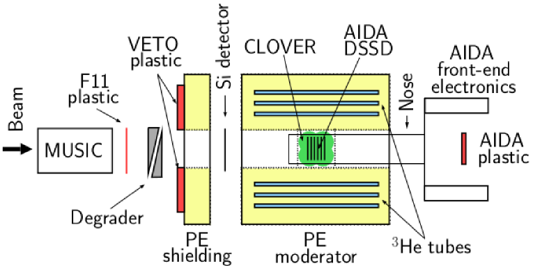
A schematic drawing of the disposition of different elements described below, belonging to the experimental setup at the end of the beam line, is shown in Fig. 1.
2.1 Measurements
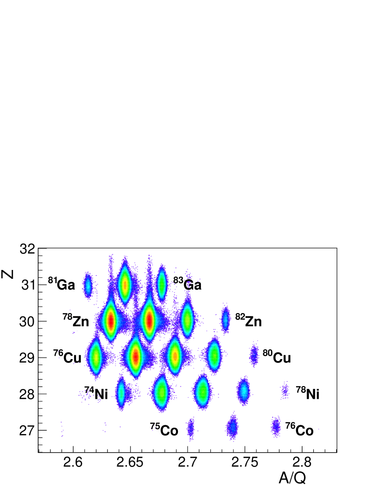
The experiments were performed using primary beams of 238U at high intensity (20-50 pnA) accelerated to an energy of 345 MeV per nucleon by the accelerator complex of the Radioactive Isotope Beam Factory (RIBF) [7]. The beam hits a beryllium target 4 mm thick producing a large number of fast reaction products which are selected by the BigRIPS in-flight separator and guided to the F11 experimental area through the Zero-Degree Spectrometer (ZDS) [8]. Each ion in the cocktail of nuclei arriving at the measuring station is identified though measurement of 1) its atomic charge Z, and 2) its mass-to-charge ratio A/Q. These quantities are obtained from the magnetic rigidity B, the time-of-flight (ToF) and the energy loss () of the ion. This information is provided by the spectrometer and its ancillary detectors: plastic scintillation detectors, position-sensitive parallel plate avalanche counters (PPAC) and multi-sampling ionization chambers (MUSIC). The last elements of the beam line were a pair of MUSIC detectors and a thin (1 mm thick) plastic scintillation detector (F11 plastic) with an area of (see Fig. 1). The ions of interest were implanted in the AIDA detector adjusting their velocity by means of an aluminum degrader of variable thickness situated after the F11 plastic. An identification plot of the ions implanted in AIDA during the commissioning run is shown in Fig. 2. The setting of the BigRIPS spectrometer was centered on 76Ni. Neutron-rich isotopes from cobalt to gallium were implanted, most of which are -delayed neutron emitters. This included 475 events for the doubly magic 78Ni.
2.2 Setup and instrumentation
The implantation detector AIDA [9] consists of a stack of six silicon double-sided strip detectors (DSSD) with a spacing of 10 mm between them. The PCB frame of the DSSD is suspended at the corners on thin titanium rods inside the AIDA nose made of 1 mm thick aluminum with a cross-section of . The nose is closed on the beam side by an aluminized Mylar foil to ensure light tightness. Each DSSD has a thickness of 1 mm and an area of , with 128 strips 0.51 mm wide on each side. The strips on the two sides are perpendicular to each other and provide high resolution position information in the horizontal (X) and vertical (Y) directions. Specially made flat cables running inside the nose bring the strip signals to the front-end readout electronics located about 70 cm away. Dual electronic chains are used to process the signals from each strip. The low-gain branch (20 GeV range) is used to process the high energy implantation signals. The high-gain branch (20 MeV range) is used to identify the much lower energy signals from particles emitted in the decay of the radioactive ions. The dual electronic processing, implemented using ASICs, minimizes the overload recovery time for registration to a few s. The stack of Si DSSDs is positioned at the geometrical centre of the neutron detector with the electronics located outside, downstream in the beam direction. A plastic scintillation detector of thickness 10 mm (AIDA plastic) is positioned on the beam axis 120 cm downstream of the stack to detect particles that pass through.
During the experiments in October-November 2017 the AIDA detector was replaced by the WA3ABi detector [10] which consists of a stack of four Si DSSDs with 3 mm wide strips. The advantage is that these DSSDs are narrower () allowing us to move the CLOVER detectors closer and increase the detection efficiency. In addition we used a new implantation-decay detector made of YSO scintillation material developed at the University of Tennessee [11, 12]. This detector consists of an array of closely packed crystals with dimension . The array is coupled through a light guide to a H8500B flat panel type photomultiplier tube (PMT) with an segmented anode that is readout with a resistor network. Both detectors were used at the same time with WA3ABi positioned off-centre mm upstream and the YSO detector positioned off-centre mm downstream. A full description of this implantation-decay setup and its performance will be given in a forthcoming publication.
During the May-June 2017 experiments we added a thin large area Si detector to the setup. The purpose of this detector is to help in the identification of light particles (p, d, , …) coming with the beam. It is a single sided strip detector of quasi-rectangular shape and dimension with a thickness of 330 m. It has 26 horizontal strips combined into two readout channels (top and bottom). The detector was placed about 50 cm upstream before the neutron detector.
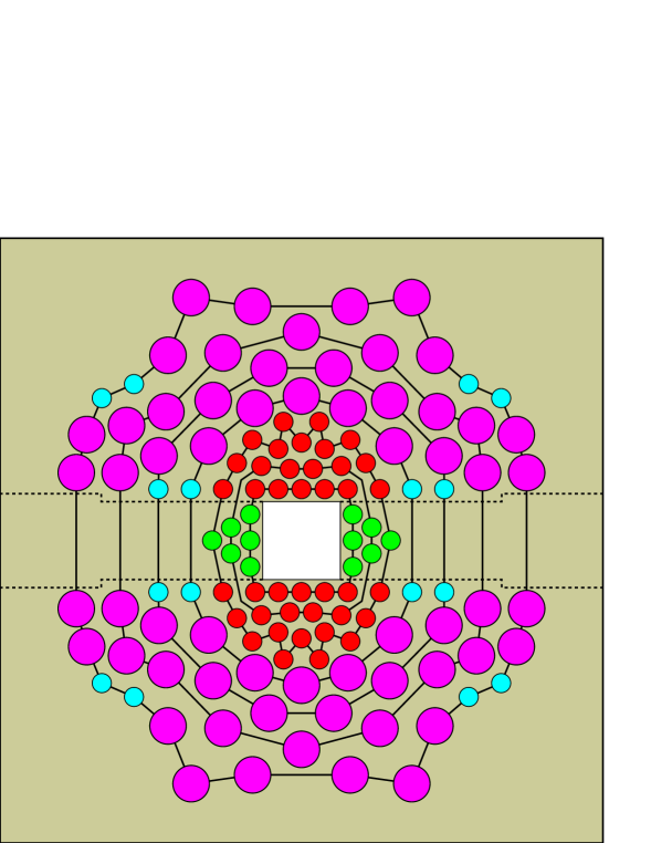
The BRIKEN neutron counter consists of an array of 140 3He filled proportional tubes embedded in a large volume of polyethylene (PE) acting as a neutron energy moderator. Very low-energy neutrons have a large interaction probability with the gas in the tubes through the reaction . This reaction liberates an energy of 764 keV that is easily detected. The PE moderator has external dimensions of , with a longitudinal hole (in the beam direction) of cross-section into which AIDA is inserted from the back. The PE moderator is constructed as a stack of 5 cm thick slabs in the longitudinal direction held together by stainless steel rods passing through the corners. The lateral sides and the top of the PE volume are covered with 1 mm thick Cd sheets and additional slabs of PE of 25 mm for neutron background attenuation. The two CLOVER detectors are inserted horizontally from opposite sides into transverse holes of cross-section facing the stack of DSSDs. Four different types of 3He tube were used in the array and their characteristics are summarized in Table 1. The UPC tubes come from the BELEN detector [13] and the ORNL tubes come from the 3Hen detector [14]. The RIKEN and ORNL tubes were manufactured by GE Reuter Stokes [15] and the UPC tubes by LND Inc [16]. The 60 cm long UPC, ORNL1 and ORNL2 tubes are arranged around the AIDA hole and are centred longitudinally on the DSSD stack. The shorter RIKEN tubes (30 cm) are disposed on both sides of each CLOVER detector hole. The transverse position distribution of the tubes is symmetrical and follows an approximate ring geometry as indicated in Fig. 3.
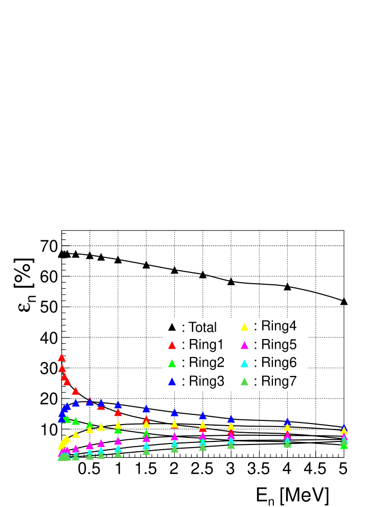
We have calculated the efficiency of the neutron detector with Monte Carlo (MC) simulations using the Geant4 Simulation Toolkit [17]. Figure 4 shows the total efficiency and the efficiency per ring as a function of neutron energy. Up to 0.5 MeV the total efficiency varies within and has an average value of 67.2%. The efficiency decreases to 65.5% at 1 MeV, then drops to 60.6% at 2.5 MeV and 51.9% at 5 MeV. We used experimental neutron spectra [18, 19] to simulate average efficiencies for a few known -delayed neutron emitters with values between 2 MeV and 5.8 MeV. The resulting efficiencies vary from 67.2% to 66.1%. A similar simulation was made using the known spectrum of 252Cf [20] extending up to 20 MeV with an average energy of MeV and a value of 61.8% was obtained . This value agrees well with the experimental result of 61.4(17)% obtained during the characterization of the BRIKEN neutron counter with a 252Cf source [21]. From these results we set the nominal neutron detection efficiency of the counter in the present configuration for isotopes with low or moderate windows to . This value is further investigated below (Section 5) using the results of measurements presented here.
| Type | Length | Diameter | Pressure | Number |
|---|---|---|---|---|
| (mm) | (mm) | (atm) | ||
| RIKEN | 300 | 25.4 | 5 | 24 |
| UPC | 600 | 25.4 | 8 | 40 |
| ORNL1 | 609.6 | 25.4 | 10 | 16 |
| ORNL2 | 609.6 | 50.8 | 10 | 60 |
We placed a PE shielding against fast neutrons coming from the beam line approximately 60 cm upstream of the neutron detector. The shielding has a thickness of 20 cm, a cross-section of and a central hole for the beam of . Cadmium sheets were fastened to the back of the shielding. At the front of the shielding two large plastic scintillation detectors were attached, above and below the hole, with dimensions . These detectors serve to discriminate against fast neutrons from the beam (VETO plastics).
The 3He tubes are connected to the preamplifiers via double-shielded coaxial cables to minimize noise pickup. These are Mesytec MPR-16-HV modules with 16 independent channels [22]. A total of 10 modules are used to accommodate all the tubes. Four of them have a differential output and the remainder have unipolar outputs. Before being sent to the sampling digitizer modules, the differential signals are converted into unipolar signals using 16 channel converter cards designed at the Accelerator Laboratory of the University of Jyväskylä (JYFL). A common high voltage (HV) is applied to all the tubes connected to a preamplifier module using a remotely controllable MPOD system from Wiener with ISEG HV cards [23]. The slow control system for this and other ancillary instrumentation was developed at ORNL (C. J. Gross and N. T. Brewer). The voltages applied are 1450 V for RIKEN and UPC tubes, 1350 V for ORNL1 tubes , and 1750 V for ORNL2 tubes. A common pulser signal is fed to all preamplifier modules. The pulse generator is driven by a precision clock running at 10 Hz. One of the pulser signals is sent directly to a free digitizer channel. The pulser is used to determine the data acquisition live time accurately.
The CLOVER detectors come from the CLARION array of Oak Ridge National Laboratory [24]. The four crystals in each detector have a diameter of 50 mm and a length around 80 mm. They are assembled inside the Al nose at 10 mm from the front face. The nose has a section of . We use the preamplified signals from the central contacts (eight in total) which are sent directly to a digitizer module. The HV is provided by the MPOD system.
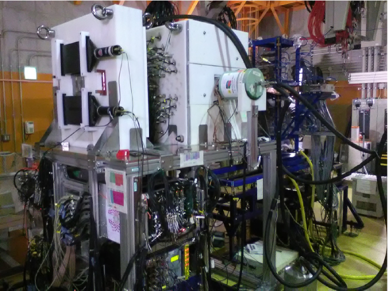
A picture of the full setup can be seen in Fig. 5.
2.3 Data acquisition and sorting
Both the AIDA detector and the BigRIPS spectrometer have their proprietary data acquisition systems (DACQ).
For the BRIKEN neutron counter we used the self-triggered Gasific DACQ developed at IFIC (Valencia) [25]. An upgrade was needed in order to handle the large number of electronic channels. The new system uses two VME crates to accommodate seven SIS3316 and seven SIS3302 sampling digitizers from Struck [26]. The SIS3316 features 16 digitizer channels, with 14 bits and a maximum sampling rate of 250 MS/s, while the SIS3302 has 8 digitizers channels with 16 bits and a maximum 100 MS/s sampling rate. For each channel amplitude and time information are registered for signals above a specified threshold. A common clock distributor SIS3820 is used to synchronize the sampling in all the modules. The clock frequency was set to 50 MHz. It is also possible to run some of the digitizers at a multiple of that frequency using a special feature of the firmware, which is an advantage when combining fast and slow detectors. The Gasific DACQ also handles the electronic pulses from the CLOVER detectors and other ancillary detectors such as the F11 plastic detector, the AIDA plastic detector, the VETO plastic detectors and the Si detector. It was also used to acquire the fast signals from the YSO detector at 250 MS/s, using the upscaling of the sampling rate feature in the DACQ. The signals from the fast plastic detectors were shaped before entering the digitizer. The digitized signals are processed on-board with a fast trapezoidal filter providing noise discrimination and timing information. Accepted signals are timestamped and processed with a trapezoidal filter with compensation for the preamplifier decay constant to obtain the amplitude (energy) information. The parameters of both digital filters are optimized for every detector type. Parameter setting, acquisition control and on-line data surveillance is performed by Gasific.
To perform a complete data analysis it is necessary to combine the information from the three independent DACQs: BigRIPS, AIDA and BRIKEN. This is done on the basis of the absolute time-stamps, thanks to the use of a common synchronization signal distributed to all three systems. Since maintaining the synchronization is crucial for the success of the measurement, we developed an on-line monitoring program that periodically spies on the timestamps on the three data streams and checks that the events are synchronized.
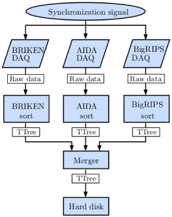
We developed an efficient scheme for data processing which gives us the possibility of performing a detailed off-line analysis with information from the three systems within a few hours (near-line analysis). This allows us to asses the progress of the measurement and to detect experimental issues that need corrective action. The scheme is shown in Fig. 6. A new run is started every hour and the data from the previous run is copied to a dedicated server. The raw data from every detector system are then processed with a specific sorting program which generates a ROOT TTree [27] file from each data stream. These TTrees contain for each event type the necessary information. The minimum information required, apart from the time-stamp, consists of: 1) BigRIPS: the Z and A/Q of each ion, 2) AIDA: the X, Y, Z position and the energy E of each ion or signal, and 3) BRIKEN: a detector identifier and the energy E of each signal.
To combine the information of the three TTrees in a single TTree a Merger software program has been developed. The program uses C++ containers to efficiently merge and order the data by time. It can also associate ROOT vectors with each output event, containing presorted time ordered data of different event types. This boosts the construction of time correlations in the off-line analysis. For example, each event can have a vector of implant events and a vector of neutron events occurring within specified time ranges around the event.
2.4 Detector performance
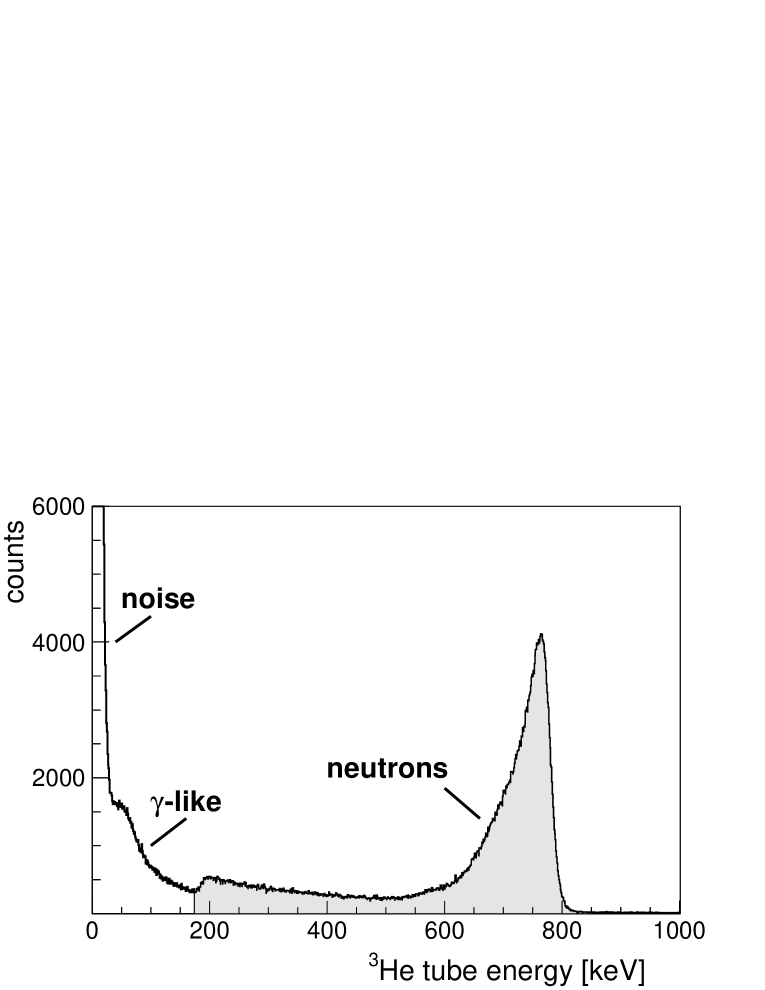
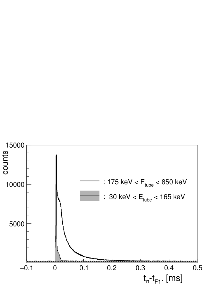
Figure 7 shows the energy spectrum registered in the 3He tubes during one run with beam. The shape of the tube response to neutrons, represented by the shadowed area, is the sum of all tube dependent responses. The characteristic full absorption peak at 764 keV serves to calibrate in energy all the tubes at the beginning of the run. In general the gain of the tubes is very stable during the measurement, with occasional minor jumps for some of them that do not even require a gain correction. The resolution and the tail produced by the wall effect determine the range of signals identified as neutrons: 175 keV - 850 keV. The data represented in the spectrum of Fig. 7 was taken with a very low acquisition threshold. The peak observed below 30 keV is dominated by electronic noise. Above 30 keV another component is seen, that we call -like. We associate this component with radiation induced by the beam on different material elements in its path close to the neutron detector. It extends well into the neutron signal range, thereby contributing to the accidental neutron background. See also the discussion related to Fig. 9 below. We found that the LND tubes are less sensitive than GE tubes to this background contribution which otherwise shows a radial intensity profile decreasing with distance from the beam axis.
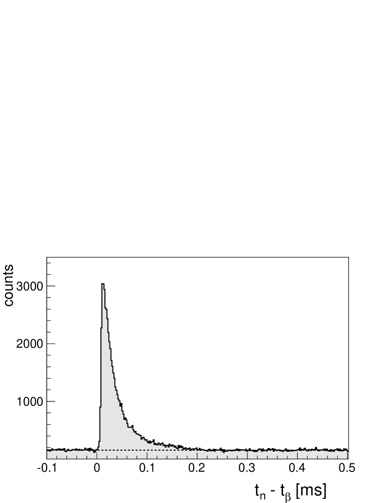
The neutron energy moderation process plus the time needed for a thermalized neutron to be absorbed in a 3He tube introduce a considerable delay between neutron production and its detection. Figure 8 shows the time distribution between neutron signals in the whole BRIKEN detector and signals identified as particles in AIDA. The tail of the distribution shows more than one exponential component but is essentially contained within the interval of 200 s (99.6%). Compared with other neutron counters of the same kind (see for example Ref. [13]) this distribution is rather short. This is a consequence of the close packing of tubes in our arrangement. Based on the moderation plus capture time spectrum we decided to use a -neutron coincidence time window of s to correlate neutrons with decays. Shorter windows could be used to reduce the ratio of accidentally correlated neutrons, represented by the flat background in Fig. 8, at the price of reducing the neutron detection efficiency.
The long coincidence window of 200 s would introduce unnecessary common dead-time in a triggered event based DACQ. This is the main reason to use our DACQ where every individual channel runs in self-triggered mode. We determine the life-time for every channel as the ratio of counts in the pulser peak appearing in the 3He energy spectrum (located outside the range shown in Fig. 7) to the pulser counts registered in an independent channel where the pulser signals are directly connected. In general we observe a very small dead-time. For example during a measurement with a 252Cf source the total rate in BRIKEN was 15730 cps, including noise. The rate per tube varies strongly depending on the position of the tube. The highest channel rate amounted to 255 cps and the lowest to 11 cps. The measured channel dead-time fractions were 0.40% and 0.01% respectively. These numbers agree well with the estimation for a non-paralyzable system using the channel trigger gate length set via software. The global dead-time is 0.36%, obtained by weighting the channel dead-times with their relative contribution to the total number of counts. In comparison, an event-based DACQ with a 200 s gate will have a dead-time of 76% at a rate of 15.7 kcps. During the experimental runs the rate in BRIKEN was never higher than a few hundred counts-per-second thus the acquisition dead-time corrections are negligible (%).
One of the issues encountered during the commissioning run was the large rate of beam induced neutrons, dominating the neutron background in BRIKEN. This came as no surprise since in a previous experiment [28] with the BELEN neutron detector at the GSI Fragment Separator (FRS) we observed in some cases more than 250 neutrons/s. The large background rate is a consequence of the high energy of the radioactive beam. We found the neutron rate at BigRIPS to be sensitive to the spectrometer setting and to the amount of material in the beam path, in particular close to the detector. Whenever possible we tried to move the material away from the experimental area. For example reducing the secondary beam energy in the early stages of the spectrometer allows us to reduce the thickness of the variable degrader controlling the implantation. In spite of these measures the observed rate is still large. During the commissioning run we measured up to 200 neutrons/s and in later experiments up to 160 neutrons/s. For comparison the rate induced by the natural background is 0.4 neutrons/s. This quite low rate is a consequence of the location of the experimental area, around 20 m underground.
We observed that a large fraction of background neutrons is time correlated with the signals of ions passing through the F11 plastic. Figure 9 shows the correlation time distribution, where the characteristic neutron moderation curve is seen. When comparing this figure with Fig. 8 two differences can be seen: the spike at and the longer tail of the distribution. The spike is due to -like signals within the neutron signal range. This is demonstrated by the grey filled histogram in Fig. 7 obtained gating on signals in the tubes above the noise but below 165 keV. The longer moderation time observed in Fig. 9, up to 500 s, is likely to be the consequence of the high energy and direction of incidence of beam background neutrons.
We exploited this correlation to reduce the neutron background effect by imposing off-line a veto condition whenever a neutron is preceded a short time before by an ion signal in the F11 plastic. This veto condition introduces an analysis dead-time that is proportional to the rate in the F11 plastic. During the commissioning run the rate in the F11 plastic was 460 cps in average, thus we decided to use a veto time window of s which captures 96.4% of background signals and gives a veto dead-time of 8.79%.
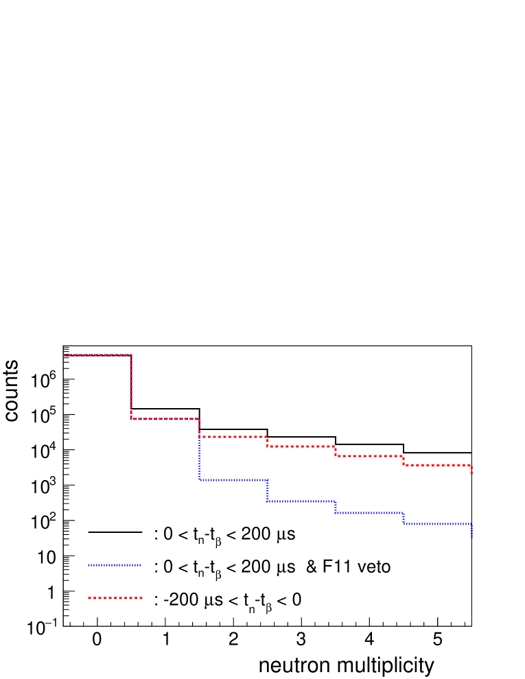
We also observed that the beam-induced neutron background has a large multiplicity (number of tubes firing). This can be a limitation for the measurement of multiple neutron emission probabilities. Figure 10 shows the observed multiplicity distribution of neutrons coming within after a signal during the commissioning run (black continuous line). It should be noted that in this run no multiple neutron emitters were produced. The figure also shows the multiplicity histogram obtained when the coincidence window is set before the signal, representing the accidentally correlated neutrons (red dashed line). In this distribution the high multiplicity of background neutrons is clearly seen: and 3 are 30% and 16% respectively of . When the F11 plastic veto condition is applied a strong reduction of the higher multiplicities is obtained as observed in Fig. 10 (dotted blue line). The reduction factor is for , for , and for , demonstrating the usefulness of the veto. A similar veto condition using the AIDA plastic detector can be added as well. This will reduce the neutron background contribution associated with light particles in the beam that go through AIDA. Light particles remain undetected in the F11 plastic because of the small thickness of this detector. For the run during May-June 2017 the addition of the AIDA plastic veto condition yields a 20% further reduction of the background. In later experiments with heavier beams the impact is larger. During the commissioning run the AIDA plastic veto condition had no significant impact. Likewise we found no significant reduction of the background vetoing with signals from the VETO plastic detectors attached to the PE shielding.
In spite of the reduction, the large rate of background neutrons prevents us from using direct neutron counting in the analysis. Decay neutron signals are buried in the background or result in a low accuracy. Therefore we have to rely on additional -gating as a way to improve the signal-to-background ratio.
3 Analysis methodology for the extraction of and
The main goal of the analysis of BRIKEN data is to extract accurately the neutron emission probability and half-life characterizing the decay of the implanted nuclei. Actually both quantities come from the same analysis procedure, although sometimes is already known from previous measurements with sufficient accuracy and only needs to be determined. This is a favorable situation because it reduces the uncertainty of the result.
To extract we need to quantify, for a given implanted nucleus, the number of decays followed by the emission of neutrons and compare it with the total number of decays. Since we do not know when an implanted ion is going to decay, we can only associate decays with implants statistically by constructing spatial and temporal correlations. Thus for each identified implanted ion we construct the histogram of time differences with all events occurring within the same spatial location and within a specified time range. The truly correlated decays will stand out from a flat background of uncorrelated decays. To assess the probability of decays we need an additional histogram similar to the previous one but adding the condition that one neutron, and only one, was detected after the within the moderation-plus-capture time (s). For decays we introduce another histogram with the condition that two neutrons are detected within after the particle. And similarly for any other decay.
However, these histograms contain not only the counts from parent decays but also from all descendants, in the case of , from descendants in the decay chain that are emitters in the case of , and so forth. Thus to disentangle the parent and descendant contributions we must fit the histograms using the appropriate solution of the Bateman equations which describe the time evolution of all activities. We use the generic form of the solution proposed in [29] which in our case simplifies to:
| (1) |
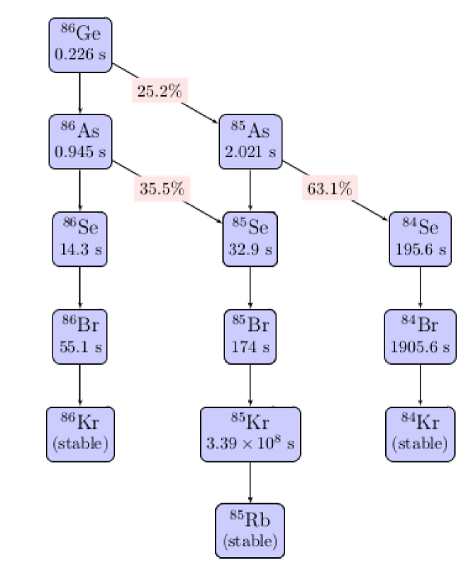
is the number of -type nuclei in a given decay path at time , is the initial number of implanted parent nuclei, and is the decay constant. The branching ratio from nucleus to nucleus in the decay chain defines the decay path. In general these branchings are just the with . In the presence of isomers with sufficiently long half-life that de-excite with a certain probability by internal transition (IT), the corresponding branching (decay path) must be included also. A typical decay network with various branching points is represented in Fig. 11.
Obviously the fit function must also include the and neutron detection efficiencies. As discussed in [25] both efficiencies are energy dependent. The efficiency depends on the end-point energy, , and the neutron efficiency depends on the neutron energy, . For the implant- time histogram the fit function takes the form:
| (2) |
Here the summation runs over the parent and all decay descendants. Since several decay paths can run through a given nucleus we must keep proper accounting of the inventory when computing using Eq. 1. The detection efficiency for the nucleus is represented by . The bar symbol emphasizes that it is obtained as a weighted average with the -intensity distribution expressed as (dropping the index for clarity):
| (3) |
Since and vary from one nucleus to another, the average detection efficiency is nucleus dependent as indicated in Eq. 2.
For the histogram the fit function takes the form:
| (4) |
Here the summation runs over the parent and all descendants that are emitters. The efficiency in the channel is averaged in the excitation energy range and is weighted by the intensity leading to emission , thus it is different from for the same nucleus:
| (5) |
The average neutron efficiency is weighted by the neutron energy spectrum :
| (6) |
For the histogram the fit function takes the form:
| (7) |
The summation runs over the parent and all descendants that are emitters, and the average and neutron detection efficiencies for the channel take the form:
| (8) |
| (9) |
Note that is the efficiency for detection of one neutron from the channel. For simplicity of notation in Eq. 7 we assume that is the same for the two neutrons emitted, i.e. they have the same neutron intensity distribution.
From the definitions above it is clear that and that . The formulae can be extended easily to , , … decays.
The fact that all average and neutron efficiencies are in principle different represents a challenge when extracting and from the fit. There is no clear way to determine these efficiencies for most of the decays, since the intensity distributions and neutron energy spectra are not known. In some cases there are general arguments, related to the size of the decay windows and expected shape of the intensity distributions, that allow us to assume that all efficiencies are equal and/or all neutron efficiencies are equal. In this situation factors out and only is needed to perform the fit. However this assumption can introduce systematic errors that need to be studied and quantified. Examples of this will be presented later.
One can see from the form of Eq. 2, 4, and 7, that the parent decay half-life intervenes in the shape of the three histograms , and . The same is true for and which appear explicitly in the last two equations, but implicitly in all three through the parent decay branchings (, see Eq. 1) that determine the weight of the respective descendant decays. The best way to take into account these correlations is to perform a simultaneous fit to all three histograms, where the unknown , , … and are the parameters of the fit. An additional fit parameter representing the normalization is always needed. This is , the initial number of implanted parent nuclei. However, before the fit can be performed we must take into account various background contributions to the experimental histograms, as explained in the next Section.
4 Background correction
A number of background sources affect the experimental histograms and . Signals identified as signals in AIDA which are not related to the decay of the implanted nucleus contribute to the accidental background. It affects all histograms and has a flat time distribution. This uncorrelated background comes from: 1) particles belonging to the decay chain of other nuclei implanted in the same correlation area, 2) light particles that pass through the detector and leave an energy similar to particles, 3) detector noise. This background component imposes a limit on the minimum detectable activity and can be reduced by optimizing the implant- correlation area, vetoing the signals correlated with the AIDA plastic, and reducing noise and optimizing thresholds in AIDA.
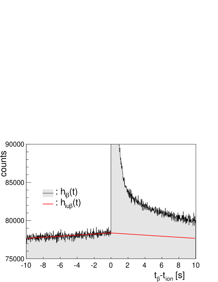
Our way to determine this background component is to: 1) construct backwards in time implant- correlations (), where only the uncorrelated particles contribute, and 2) extrapolate to positive times. An example of this is shown in Fig. 12 showing the histogram for 83Ga in the time range . As can be seen, the background time distribution is not constant for and has a small positive slope. This effect could be traced back to accidental beam interruptions during a run, when the rate decreases. During the commissioning experiment there were frequent beam interruptions (instabilities) lasting from less than a second to few tens of seconds. We verified that removing from the time correlation the data coming up to 10 s before and after a beam interruption the uncorrelated background becomes nearly constant reducing the statistics by a factor of 2. Using MC simulations we verified that the background shape depends on half-lives and length of the interruption. For a random distribution of interruption intervals we obtained a background shape that is symmetrical around t=0 to a good approximation, thus we take this assumption in our analysis (see Fig. 12). It is worth to mention that the analysis of the data obtained removing beam interruptions gives the same result within statistics than the full data set (see Section 5). We observe that in most of the cases a linear function provides a good reproduction of the uncorrelated background. On occasions an exponential function reproduces the shape better. In either case they define the correction histograms and .
In the case of the histogram this is the only background contribution thus the relation of the measured histogram to the unperturbed time distribution (see Eq. 2) is given by:
| (10) |
Another important source of background comes from neutrons that are accidentally correlated with particles within the time window for -neutron correlation . This only affects the histograms. Neutron signals that can be accidentally correlated come from: 1) neutrons emitted by other implanted nuclei, 2) beam induced neutrons, 3) ambient background neutrons, and 4) detector noise, including -like signals in 3He tubes. This background component affects the minimum detectable activity and can be minimized with proper detector shielding, discrimination of beam induced neutron signals and detector noise reduction. A characteristic of this type of background is that it follows the time distribution of implant- correlations and thus it has a time structure. This has a direct impact on the extraction of and from the fit and it is crucial to have an accurate method of background correction.
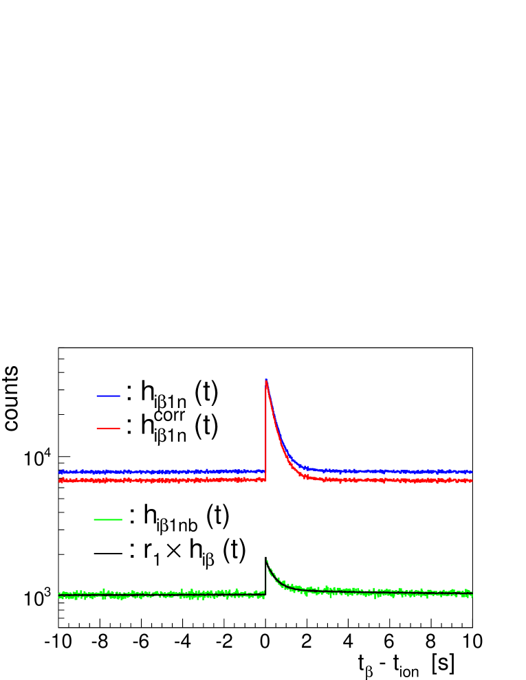
We introduce here a new method of correction for accidental -neutron background that estimates accurately its contribution directly from the data. Figures 13 and 14 show the relevant histograms for the discussion in the example of 83Ga decay. In this case we use the data taken during the May-June 2017 run, which has much higher statistics ( implanted ions) to demonstrate the results.
The method is based on the use of backwards in time -neutron correlations to determine the number of accidental neutrons correlated with particles. The idea is that the number of accidental neutrons coming within after the is on average the same as the number of neutrons coming within before the , all of which are of necessity accidentals. The only assumption here is that the neutron background rate is not changing, on average, over a period of a few hundreds of s. We construct a new implant- time correlation histogram with the condition that one neutron arrives within before the . This histogram, that we designate is shown in Fig. 13 in green. Notice that the shape of this histogram is identical to the scaled histogram represented in black in the figure. The scaling factor :
| (11) |
is the probability of having one-accidental-neutron per detected , determined with great precision because we use the full statistics of the histograms. In the present example . The value of changes by a few percent from one nucleus to another due to changes in the relative background conditions. For example a nucleus with high implantation rate and large sees less background than a nucleus with low implantation rate and small .
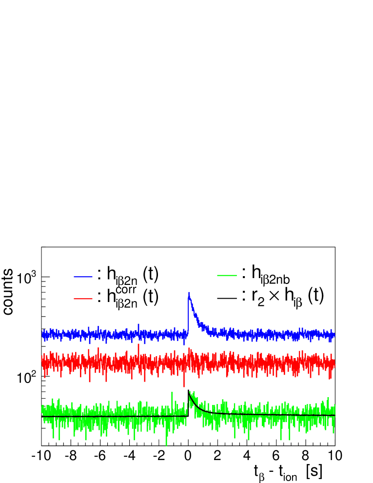
We also construct , the implant- time correlation histogram with the condition that two neutrons are coming within before the . This is shown in green in Fig. 14 and as before its shape is matched by the scaled histogram (in black). The scaling factor :
| (12) |
represents the probability of having two-accidental-neutrons per detected . In the present example , twenty five times smaller than . A similar procedure can be applied for higher accidental neutron multiplicities. The red-dashed histogram in Fig. 10, representing the multiplicity of neutrons accidentally correlated with a particle, give us information about the value of for . The total probability of accidental neutrons per detected is .
Let us consider the case of decays followed by one-neutron emission. The measured histogram is represented in blue in Fig. 13. This histogram has to be corrected for background contributions to obtain the unperturbed time distribution represented by the function defined in Eq. 4. Accidental neutron coincidences have two effects on this distribution. One effect is a loss of counts whenever one or more background neutrons comes accidentally within after the in addition to the truly correlated neutron. The loss is proportional to the total probability of accidental neutrons per detected . The net effect is a scaling down of the distribution, of the form . The other effect is the appearance of spurious counts in the histogram when one accidental neutron correlates with particles that do not see correlations with decay neutrons. The latter have a time distribution that can be obtained as the difference between the distribution of all detected events, , and the distribution of events where one decay neutron was detected, . Scaling this distribution by , the probability of one-accidental-neutron per , gives the contribution . The measured histogram is then the sum of both terms plus the uncorrelated background contribution . After some rearrangement it gives:
| (13) |
To visualize the size of the corrections it is useful to calculate the histogram that is shown in red in Fig. 13. Note that both and include their respective uncorrelated backgrounds. As can be seen in Fig. 13 the correction is small in this case but it would be important if the value is small. An example will be shown later.
Let us turn now to the case of two-neutron emission. The measured histogram is represented in blue in Fig. 14. This histogram has to be corrected for background contributions to obtain the unperturbed time distribution represented by the function defined in Eq. 7. The effect of accidental coincidences with background neutrons in this histogram is similar to the one explained above: loss of true counts and appearance of spurious counts. In addition one has to modify the corrections to the histogram (Eq. 13) to take into account the contribution of the 2n decay channel [30]. In A we explain in detail how to obtain the different correction terms. Here we simply give the result expressed as the relation between the measured histograms and and the unperturbed time distributions , and :
| (14) |
| (15) |
where .
The computation of the background corrected implant--1n and implant--2n histograms from the measured histograms gets more complicated now because of the interdependence of the corrections. We give in A the appropriate formulas. In the present example, the corrected histogram is represented in red in Fig. 14. As can be observed the peak in the uncorrected time distribution (blue) disappears in the corrected time distribution, which is completely flat. This agrees with the fact that 83Ga must have a extremely small due to the small MeV. It confirms the accuracy of the correction method and demonstrates the importance of accidental neutron background correction for determining small values.
Similar formulas for emitters are given in A.
We should mention that an alternative method of analysis and background correction for BRIKEN data has been developed [31]. Compared to the method presented here, this alternative method determines initial parent activities for each of the decay channels from independent fits to the corresponding time correlation histograms. These initial activities are then combined to obtain values applying global time-independent corrections for the correlated neutron background contribution.
5 Selected results
We present in this section details of the analysis for a few isotopes in order to illustrate the procedure and the quality of results.
The data was acquired during the commissioning run over 10 effective hours of measurement at a primary beam intensity of 20 pnA. In the sort of AIDA data, events are treated by defining clusters of consecutive strips firing above the noise threshold (strip dependent) in both X and Y directions. This takes into account the fact that particles can have a long range in Si. A pixel is determined by the energy weighted centroid of the cluster of strips with the condition that X and Y energies are similar. Implantation events have a small strip multiplicity (one or two strips) and are defined by the last layer (DSSD) firing the low gain electronic branch. We consider only ion- correlation events when they happen in the same layer (Z position) and the difference of X and Y centroid positions between and ion is less than three strips (defining a correlation area of ).
We discovered during the run in May-June 2017 a problem related to the design of the AIDA adaptor PCB cards that serve to connect the flat cables coming from the Si DSSD . The effect was a transient induced by implantation events in the high gain electronics which is interpreted as a event. The effect lasted up to a few tens of ms and appears as a spurious implant- time correlation extending up to 30-40 ms. These background signals can be effectively eliminated by neglecting the first 50 ms in the fit of the time correlated histograms. In the runs this is not an issue because the half-lives are relatively long. After identification of the problem the coupling cards were modified and the effect eliminated as verified during the October-November 2017 run.
5.1 Fitting procedure
We construct the time correlation histograms and for all implanted ions that are identified. We choose a time window from -10 s to +10 s that is appropriate for all the cases analyzed. The binning of the histograms for each nucleus is chosen balancing the need to have enough points to determine the activity evolution and minimize the statistical fluctuation in the bin counts.
A fitting subroutine was written using ROOT::Fit classes [27]. The inputs to the program are the measured time correlation histograms, the half-life and neutron emission probabilities of all nuclei involved and the corresponding and neutron efficiencies. All parameters have an associated uncertainty and can be fixed during the fit. The program automatically reconstructs the decay network based on the nuclei and information provided.
For the fit we do not subtract the different background contributions from the measured histograms but rather include these contributions in the fit function. See A. This is the proper way to handle the corrections in view of the use of Maximum Likelihood estimators. Histogram subtraction destroys the Poisson character of bin counts leading eventually to negative counts for low statistics. In general we use the Binned Maximum Likelihood (BML) algorithm to fit the histograms, except when the very low statistics suggest the use of the Unbinned Maximum Likelihood (UML). In this case the event data are provided in list mode. The uncorrelated -ion background is obtained from a fit to the negative time range for each of the and histograms taking into account the effect of the correlated neutron background correction histograms (see A). The fit to the positive time range skips the first few bins in order to exclude the initial 50 ms range where the ion induced background appears.
To evaluate the systematic uncertainty due to the parameters fixed during the fit (half-lives, neutron branchings, backgrounds, efficiencies) we use a Monte Carlo approach. For any chosen subset of parameters we define a multivariate normal distribution, using the adopted value of each parameter as the mean and the square of the quoted uncertainty as the variance. In general we assume that different parameters are uncorrelated (diagonal covariance matrix). The multivariate distribution is randomly sampled and the fit performed. The resulting fit parameters (, , …) are histogrammed and at the end the standard deviation of the sample distribution (eventually asymmetric) is evaluated and quoted as the systematic uncertainty.
For the fit we need to define and neutron efficiencies. We assume that the nominal value of the neutron efficiency is % as discussed in Section 2.2. This efficiency has to be renormalized in order to take into account the neutron count loss because of the finite size of the -neutron correlation window (0.43%), and the dead-time introduced in the analysis by the neutron veto from the F11 plastic detector (8.79%). This gives a value of 60.7(18)% for the effective neutron efficiency. This efficiency would have to be modified for decays with a particular hard neutron spectrum. The influence of efficiencies will be discussed in the next subsection.
5.2 Effect of efficiencies
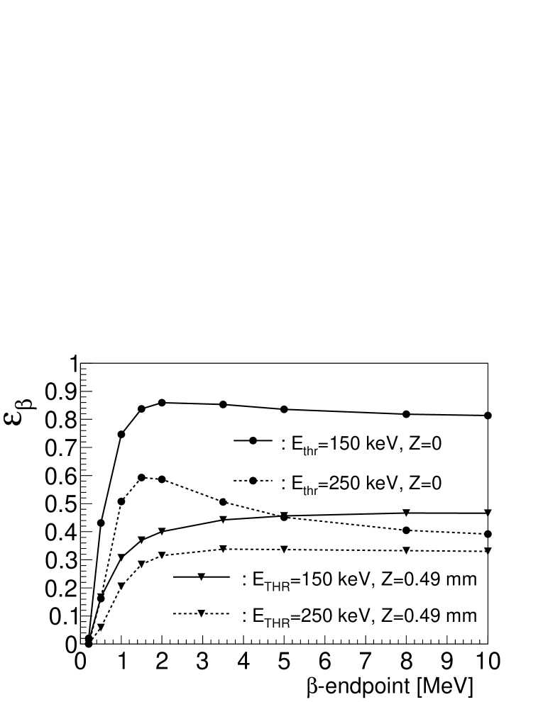
The continuum nature of the spectrum together with the unavoidable minimum electronic thresholds introduce a end-point energy dependence in the detection efficiency [25]. In the case of an implantation-decay detector like AIDA the energy dependence is further complicated with a dependence on the implantation depth and with the method of reconstructing events. To illustrate the dependence with threshold and implantation depth we show in Fig. 15 the result of Geant4 simulations using the AIDA Si DSSD geometry. This efficiency does not include the effect of event reconstruction and the absolute values are not representative of the actual efficiencies.
As can be observed in Fig. 15 there is a fast drop in the efficiency for end-point energies below MeV. When the particle is emitted from the middle of the DSSD the efficiency is quite large if the threshold is low (below about 150 keV). In this case increasing the threshold (250 keV in the example) has a substantial effect, with the efficiency dropping for increasing end-point energies. When the implantation occurs close to one of the DSSD surfaces, half of the particles have little chance of depositing enough energy and the efficiency drops. The effect of a threshold increase is smaller in this case. Because of the energy spread of implanted ions the implantation depth effect is partially smeared out. As explained in Section 3 this energy dependence can introduce differences in average efficiencies for different nuclei and decay branches, depending on the intensity distribution, which leads to systematic errors in the results of the fit. Note that the systematic effect is due to the relative differences and not to the absolute efficiency values.
It is not easy to determine experimentally the efficiency for every decay mode contributing significantly to the fit. One possibility is to use the intensity of decay -rays observed in the CLOVER detectors to obtain information on the average efficiency. This requires the comparison of -gated with ungated ray spectra [32], but it is in practice difficult to apply because of the large background and the limited statistics. Another approach is to calculate a realistic efficiency curve from Monte Carlo simulated data and use intensity distributions to compute the average efficiencies (Section 3). Since for most of the exotic decays this information is unknown or poorly known, one must rely on theoretical -strength distributions to obtain an estimate. In spite of the uncertainties inherent in this approach it can give a representative value of the size of the systematic error. A third approach is to determine the efficiencies from the time correlation data as will be discussed below.
An important consideration is that the end-point energy dependence of decreases as the threshold decreases (it disappears at threshold zero). Therefore minimizing the effective -energy threshold in AIDA data is an important requirement to minimize this kind of systematic error. One can test the magnitude of the systematic error by analyzing data obtained with different thresholds. Such a test is shown in Fig. 16 for a set of Ni, Cu, Zn and Ga isotopes measured during the commissioning run. They span ranges of MeV and MeV.
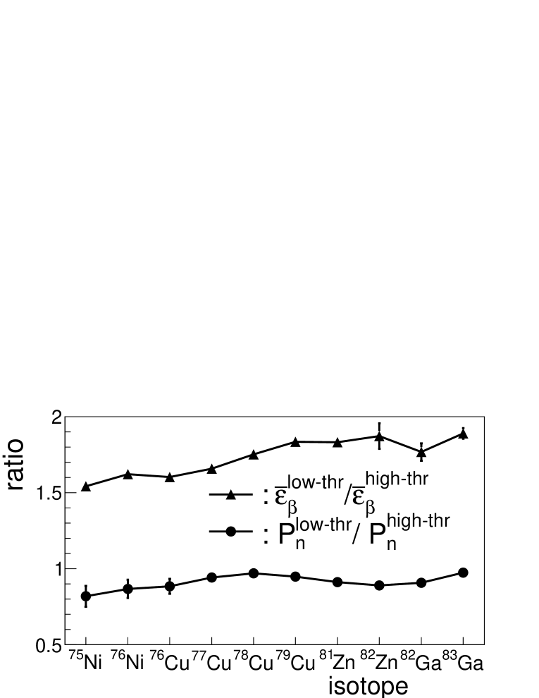
The fit to the time correlation histograms and used to extract the and efficiencies shown in Fig. 16, assumes that all are equal. In this case the efficiency factors out of the fit function (see Eq. 2 and Eq. 4) and can be determined from the result of the fit. The fit parameters are and the normalization constant, equal to . The remaining parameters are kept fixed to the adopted values in standard databases [33]. Dividing the normalization constant by determined as the number of identified implanted ions we obtain . The extracted efficiency is indicative of the effective threshold. In the sort with the low threshold the efficiencies vary between 30% and 42%. In the high threshold sort the efficiency range is 20-26%. The actual thresholds applied to AIDA data are strip dependent and vary between 100 keV and 250 keV in the high threshold sort and between 50 keV and 200 keV in the low threshold sort.
Figure 16 shows the ratio of efficiencies and the ratio of values between the low threshold sort and the high threshold sort. The low threshold increases between 54% and 89% with respect to the high threshold. The impact on is a reduction of all values by factors from 2.5% to 18%. We have not observed a clear correlation of the reduction factor with the size of the decay windows and .
Minimizing the thresholds in the AIDA sort is a challenging task because of the large number of channels and the nature of the noise, which is channel specific and time dependent. A compromise must be established between lowering the threshold and keeping a reasonable signal-to-noise ratio. For the commissioning run we adopt the low threshold sort discussed above that should reduce the effect of efficiency dependence in the data. The question is whether a residual effect still remains.
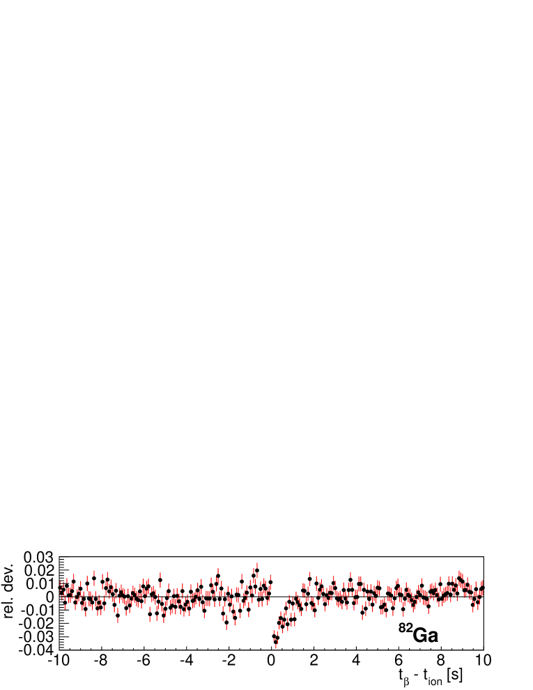
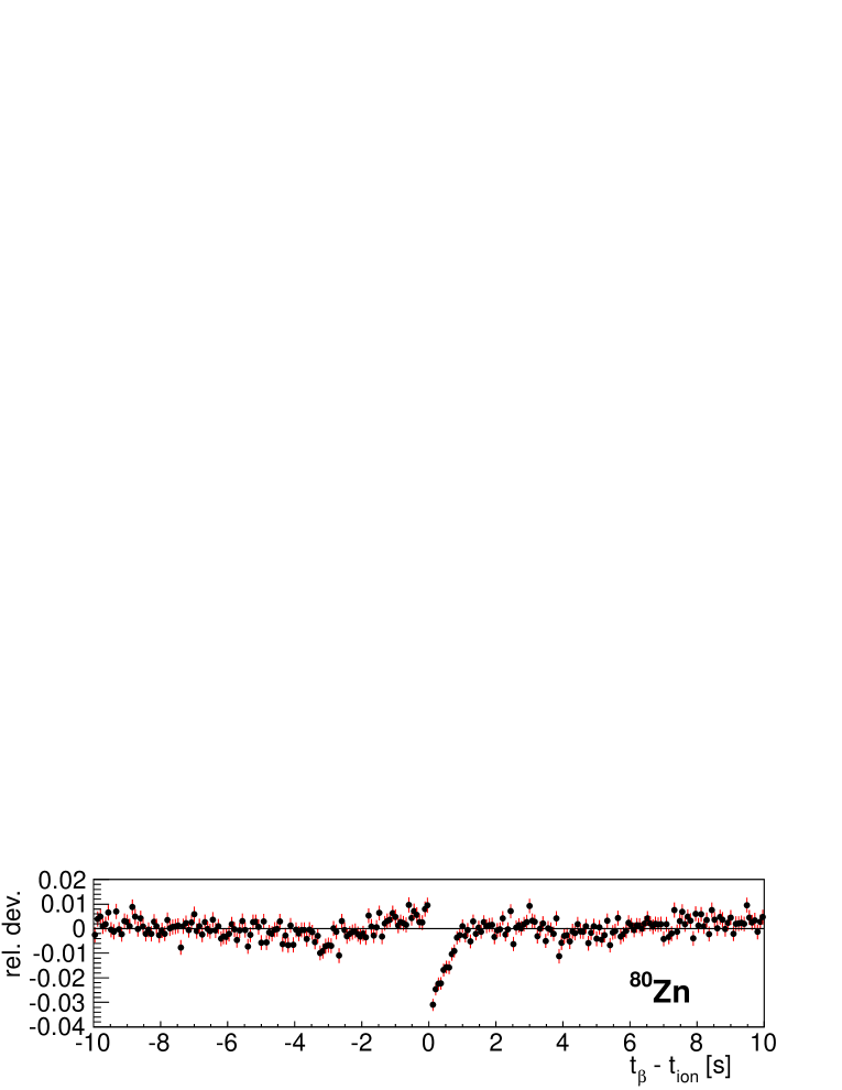
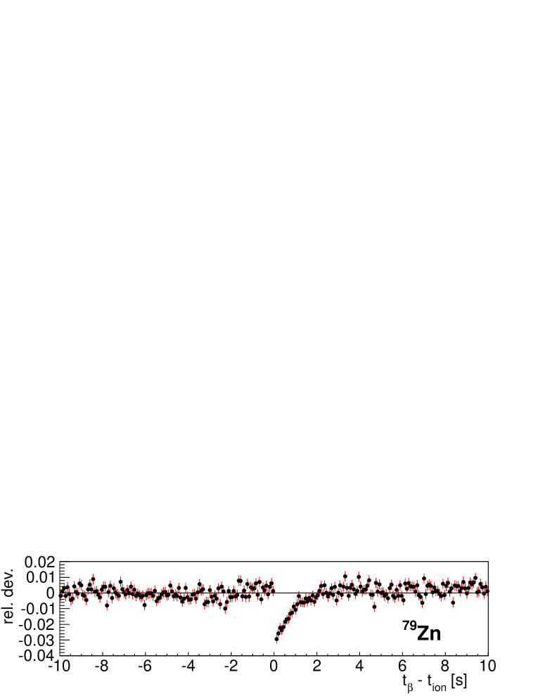
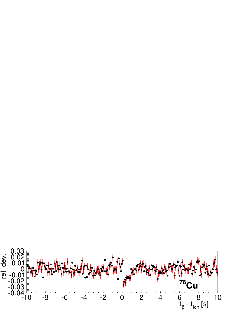
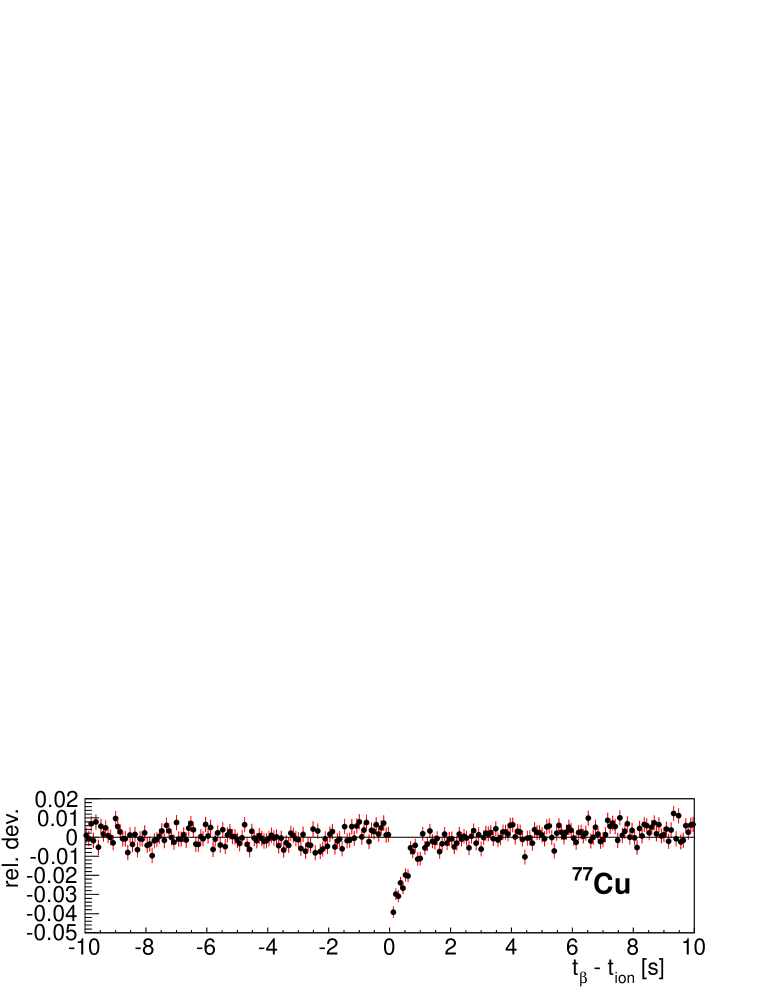
As a matter of fact we observe a small but systematic deviation between data and best fits for nuclei with high implantation statistics during the commissioning run. Figure 17 shows, relative values of fit residuals for implant- time correlation histograms . To show the effect more clearly the fit region is restricted to implant- correlation times in the range [1 s, 10 s]. As can be observed all show a similar pattern: there is a deficit of counts at short correlation times and a slight excess at long correlation times. We do not observe this effect in the fit of the neutron-gated implant- time correlation histogram . We interpret this result as a consequence of the difference in efficiency between the parent nucleus and descendants. In all cases except 80Zn, this can be related to the much larger decay window of the parent. The case of 80Zn will be commented on later.
In view of this result we will include in the fit, when necessary, as an additional adjustable parameter the relative efficiency of selected decay modes in the chain.
5.3 82Ga: verification of neutron efficiency
During the commissioning run we accumulated ions of 82Ga, a good case to verify the neutron efficiency since the for this decay is fairly well known. There are three previous measurements which give consistent values: 21.4(22)% [36], 19.8(10)% [37], and 22.2(20)% [32]. Their weighted average gives 20.4(12)%. In addition there are two values with larger uncertainty that deviate significantly from the other results, 31.1(44)% from [38] and 30(8)% from [39]. The new evaluation of and for -delayed neutron emitters fostered by the IAEA [40] recommends a value of %, obtained by a weighted average of all measurements except the first one.
82Ga is the sole neutron emitter in its entire decay network. The one-neutron emission window is MeV. This value and the values of other decay energy windows in this paper are taken from the 2016 Atomic Mass Evaluation [41]. The neutron energy spectrum has not been measured for this decay but it was for the lighter isotopes 79-81Ga [18]. From the evolution of the shape one can deduce that most of the neutron spectrum for 82Ga should be contained within 1 MeV. This is confirmed by theoretical calculations of the delayed neutron spectrum, which can be retrieved from the ENDF/B-VII.1 data base [19]. This spectrum is calculated from -strength distributions obtained within the QRPA formalism [42] and neutron emission rates obtained within the Hauser-Feshbach formalism [43]. Thus we conclude that the use of the nominal neutron efficiency (Section 2.2) should be appropriate in this decay.
Our data and the fits are shown in Fig. 18. There is a large difference between the fit and measurement at the first positive time bin in the histogram (with counts it is outside the range shown). This is caused by the ion-induced background. The corresponding histogram bin is not included in the fit region. The number of accidental one-neutron counts per detected is , much smaller than the values obtained in the May-June 2017 run (see Section 4). This reflects the different background conditions in the two experiments. In the fit all the decay branches down to stable nuclei are followed. The half-life of all descendants is relatively well known [33]. The half-life of 82Ga is also well known, ms [40], and was fixed in the fit. Ambiguities appear in the case of 81Ge with two known -decaying isomers. However, both have equal half-life within uncertainties according to [44], which minimizes the impact of the respective unknown population. Also in the case of 82As two isomers are known but the decay of the ground state of 82Ge will populate weakly the isomer and it was neglected. The case of 81Se, again with two isomers, poses no problem since it contributes marginally to the decay activity.
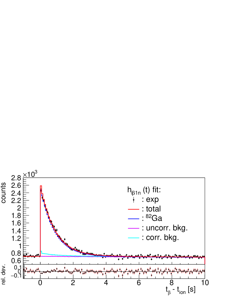
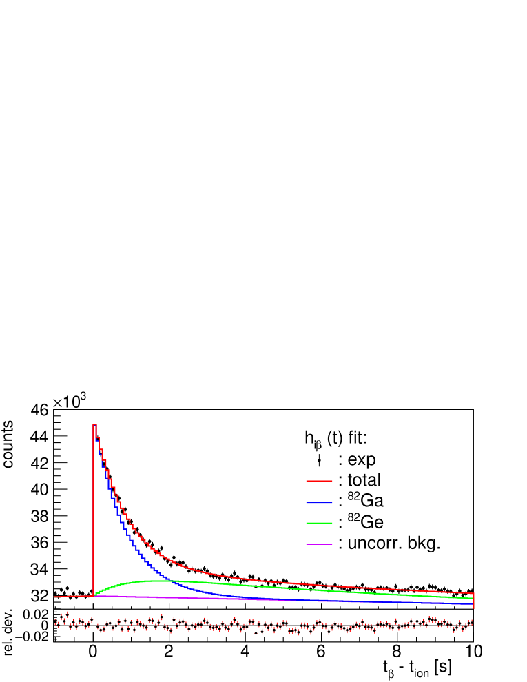
The decay energy window for 82Ga is large, MeV, much larger than the for other contributing decays. In particular it is nearly 8 MeV larger than the of the daughter 82Ge, the second largest contributor in the decay chain. Therefore the fit was performed including as a free parameter the efficiency for the parent decay, resulting in a value of %. If we keep all efficiencies fixed the fit is poorer ( instead of 0.98, see also Fig. 17) and the result becomes 13% larger %. The fitted efficiency is %, relative to the efficiency for the remaining decay branches, that are kept fixed. This can be interpreted in the light of the simulations presented in Fig. 15 showing that if on average the decay proceeds by large decay energies the efficiency can be lower than if it decays with smaller energies.
The uncertainty on values quoted above is obtained from the fit and represents the statistical uncertainty. The systematic uncertainty due to the uncertainties in the half-life of the parent and all descendants was evaluated as 0.16% using the parameter sampling procedure described before. The uncertainty due to the assumed uncertainty in the neutron efficiency amounts to 0.61%. The uncertainty due to the background corrections (correlated and uncorrelated) is evaluated as 0.18%. The total systematic uncertainty is 0.65%. Combining quadratically the statistical and systematic uncertainties our result is %. It agrees within uncertainties with the weighted average of previous measurements with the lower values [36, 37, 32] , %. The result confirms also the value of the nominal efficiency used.
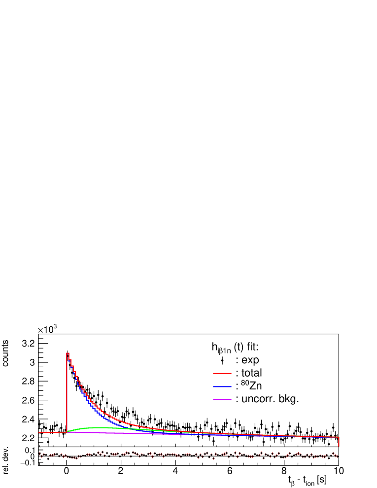
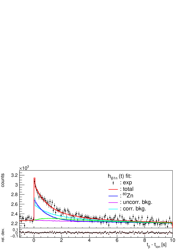
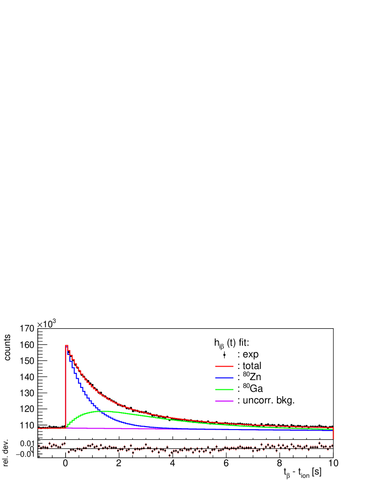
5.4 80Zn: sensitivity limit to small
The importance of a proper correction of accidentally correlated neutron background in the case of weak two-neutron emitters was demonstrated in Section 4. 80Zn with MeV and a small value is a good example of the importance of background correction for weak one-neutron emitters. It serves also as a test case to study the sensitivity limit of our experiment for determination. There are two previous measurements of the delayed neutron emission probability in 80Zn. A rather uncertain value of 1.0(5)% is reported in [45] and an upper limit, %, is reported in [39]. The new evaluation [40] adopts the value of [45].
One million 80Zn ions were implanted during the commissioning run. In the decay chain [40], 80Ga is a known -delayed neutron emitter with a weak neutron branching % and 79Ga is an even weaker emitter with %. Two isomers are known [46] in 80Ga with s and s , but the high-spin isomer is only weakly populated in the the decay of the 80Zn ground state and it was ignored. The of 80Zn, MeV, is actually smaller than that of the daughter 80Ga, MeV, at difference with the remaining cases shown in Fig. 17. Another characteristic of the decay of 80Ga is the sizable population of a state at keV that emits conversion electrons and of a state at keV that can only decay by electron conversion to the g.s. (E0 transition) [47]. These low-energy conversion electrons are easily detected in AIDA increasing the apparent efficiency for 80Ga decay. Therefore we leave this efficiency as a free parameter of the fit. The lower panel of Fig. 19 shows the good quality obtained in the fit to the histogram. The adjusted efficiency is 15% larger than the efficiency for other decay branches that are kept fixed. This result can be understood as the effect of conversion electrons.
The upper panel of Fig. 19 shows the fit to the implant--1n histogram without correction for the accidental correlated one-neutron background and the central panel the fit including the correction. As can be seen this correction represents the largest contribution to the measured histogram. Without correction the fit to is poor because the correlated background has the shape of (see Section 4) and the resulting % is too large. After correction we obtain % in agreement with previous results. A fit where all efficiencies are kept fixed results in a value of 1.28(11)%. The systematic uncertainty due to background correction is 0.06%. The one due to the fixed parameters in the fit (all and of descendants) is 0.02% and that of the neutron efficiency is 0.04%. Combining all uncertainties our final result is %.
This case shows also that rather accurate values on the order of one percent can be extracted from our data. This statement of course depends on the implantation statistics. We have tested that analyzing one tenth of the present statistics ( ions) one can still obtain a reasonable result of %.
5.5 81Ga: sensitivity limit for small implant statistics
The decay window for neutron emission in 81Ga is MeV. It is the only neutron emitter in the decay chain network. There are three previous measurements that agree relatively well: 12.0(9)% [36], 10.6(8)% [37], and 12.9(8)% [38]. The new evaluation [40] recommends the value of %. The half-life is also well known s. The number of implanted ions during the commissioning run was 4400. Thus this case serves to test the sensitivity limit of our setup with low statistics.
Figure 20 shows the result of the fit using the nominal neutron efficiency and fixing the half-life of descendants to the values in the ENSDF database [33]. The efficiencies were kept fixed during the fit. A total of 190 neutrons stand out from a background of 820 neutrons. The from the fit is 11.3(23)%. The systematic uncertainty due to parameters that are kept fixed in the fit is 1.2%. Our result is then in agreement with previous results.
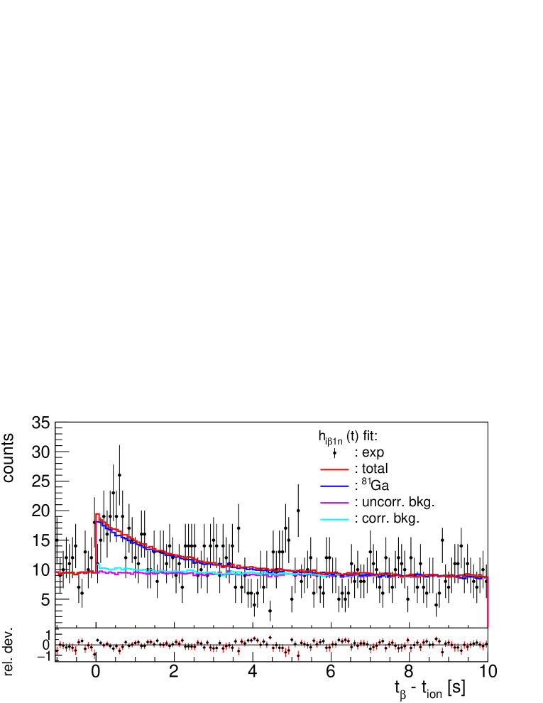
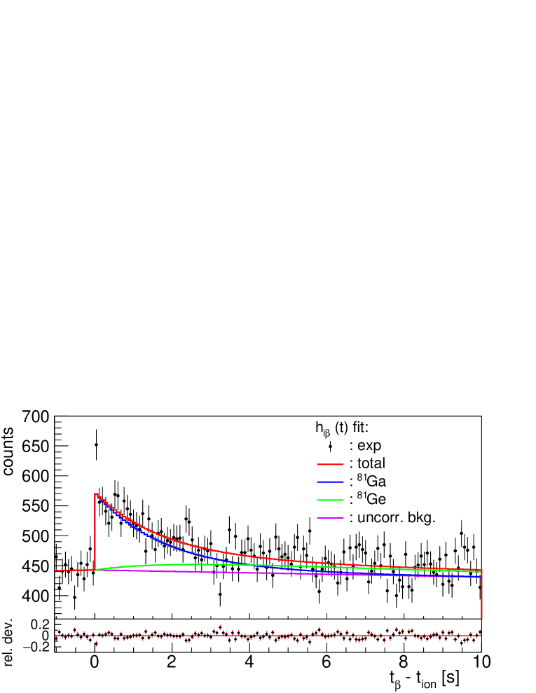
This demonstrates that with a few thousand ions we are able to measure values of the order of 5-10% with accuracies in the order of 25%.
6 Conclusion
We have carried out the commissioning of a new setup for the measurement of decay properties of -delayed neutron emitters using radioactive beams at RIKEN. This allowed us to verify the performance of the BRIKEN neutron counter under experimental conditions. We found that the beam induced neutron background in the detector is about 2-3 orders of magnitude larger than the natural neutron background. The background rate is quite sensitive to the spectrometer setting. Minimizing the material in the beam path close to the detector helps to reduce the background. We found that another effective way of reducing the background is to veto neutron signals coming shortly after any beam particle enters the experimental area. This reduces the one-neutron background rate by a factor 2-3 and the two-neutron background rate by a factor 30. The large background imposes a limit on the minimum measurable that otherwise depends on the statistics (number of implanted ions) and the value of itself. We demonstrated that we are able to determine values of the order of 1% with ions. We could determine also values of the order of 10% with few thousand implanted ions. For values the situation is more favorable because of the much higher background reduction.
Because of the large size of the -neutron coincidence window (200 s) the number of accidental -neutron correlations is large. This introduces a distortion of the -implant-neutron time correlation spectra that severely affects the determination of small and values. We have introduced a novel method, based on time-reversed correlations, to determine this distortion accurately and correct for it.
Systematic errors due to the unknown dependence of and neutron efficiency on nucleus and decay branch have been discussed. Although the design of the BRIKEN neutron counter minimizes the neutron energy dependence of the efficiency, reductions of up to about 10% with respect to the nominal neutron efficiency can be expected for decays with large windows. The correct efficiency can be calculated from the neutron spectrum and simulated efficiencies. In cases where the spectrum is unknown one can use theoretical estimates to compute the correction factor. Another possibility, that we are currently investigating, is to use the number of counts per detector ring, which is sensitive to the neutron energy distribution, to determine directly the effective average efficiency.
The evaluation of systematic errors due to differences in efficiencies is more challenging. As this effect is related to the threshold in the detector, minimization of the threshold for events in the sorting of AIDA data is a requisite for accurate determinations. This is a demanding task given the complexity of this type of detector and the varying conditions in different experiments. Currently we are actively working to improve the event reconstruction in AIDA. For the commissioning run we selected a sort that is a compromise between threshold reduction and signal-to-noise ratio. We found evidence for a residual efficiency effect in the fits to these data. These are in general cases where the parent decay is quite large, much larger than the decay energy window for other contributing decay branches. Our approach to solve this issue is to include the parent decay efficiency as an adjustable parameter in the fit. We also studied a case where the efficiency of the daughter decay is increased due to the emission of conversion electrons.
We presented the result of the analysis for few selected cases measured in the commissioning run. The results obtained for other cases will be presented in a forthcoming publication. They confirm the value of the neutron efficiency for the current setup. They show also the importance of an accurate correction of the correlated neutron background. In general they confirm the good performance of the detector setup and the expected quality of the results from the experiments that have been already performed or are planned .
Acknowledgment
This work has been supported by the Spanish Ministerio de Economía y Competitividad under grants FPA2011-24553, FPA2011-28770-C03-03, FPA2014-52823-C2-1/2, IJCI-2014-19172 and SEV-2014-0398, and by FP7/EURATOM Contract No. 605203. This work has been supported by the Office of Nuclear Physics, U. S. Department of Energy under the contract DE-AC05-00OR22725 (ORNL). This research was sponsored in part by the Office of Nuclear Physics, U.S. Department of Energy under Award No. DE-FG02-96ER40983 and by the National Nuclear Security Administration under the Stewardship Science Academic Alliances program through DOE Award No. DE-NA0002132. This work was supported by JSPS KAKENHI (Grants Numbers 14F04808, 17H06090, 25247045, 19340074). Supported by the UK Science and Technology Facilities Council. This work has been supported by the Natural Sciences and Engineering Research Council of Canada (NSERC) via the Discovery Grants SAPIN-2014-00028 and RGPAS 462257-2014. This work has been supported by the National Science Foundation grant PHY 1714153. Supported by the National Science Foundation under Grant Number PHY- 1430152 (JINA Center for the Evolution of the Elements), Grant Number PHY-1565546 (NSCL). Supported by the UK Science and Technology Facilities Council grant No. ST/N00244X/1. This work was supported by NKFIH (K120666). Supported by South Korea NRF grants 2016K1A3A7A09005575 and 2015H1A2A1030275. Work partially done within IAEA-CRP for Beta Delayed Neutron Data. G. G. Kiss acknowledges support form the Janos Bolyai research fellowship. This experiment was performed at RI Beam Factory operated by RIKEN Nishina Center and CNS, University of Tokyo.
Appendix A
We describe in this Appendix how to obtain background correction formulas for the analysis of BRIKEN data from 2n emitters. We calculate the effect of accidental coincidences with background neutrons on the measured histograms and that, together with , are needed to obtain , and . At the end of the Appendix we give also, without deduction, the corresponding formulas for the case of 3n emitters which can be obtained following a similar line of reasoning.
Let us consider first the histogram. The corresponding unperturbed time distribution is represented by the function defined in Eq. 7. As mentioned in Section 4, one of the effects of accidental coincidences with background neutrons is the loss of counts, resulting in a scaling of this distribution of the form , where is the total probability of accidental neutron coincidences per . In addition to this effect accidental coincidences produce spurious counts in the histogram that come from three different sources.
The first contribution comes from particles that do not see correlations with decay neutrons but accidentally correlate with two background neutrons coming within the coincidence window. The probability of accidental correlation with two bacground neutrons is given by , see Eq. 12. The time distribution of events that do not see correlations with decay neutrons can be obtained by subtraction from the distribution of all events, (Eq. 2), those events where decay neutrons are detected. For the 1n decay channel this is represented by (Eq. 4). For the 2n decay channel, two terms appear. The first term corresponds to events where the two neutrons are detected and is represented by . The second term corresponds to events where only one of the two neutrons is detected. The probability of detecting only one of the two neutrons emitted is given by , assuming that the neutron detection efficiency for both neutrons in the 2n channel (Eq. 9) is equal. Taking into account the dependence of (Eq. 7) with then , with , represents the distribution of events where only one neutron is detected. Taking both terms into consideration, this contribution takes the form .
The second contribution comes from events belonging to the decay channel when in addition to the detection of a decay neutron, with time distribution given by , a background neutron accidentally arrives within with probability (Eq. 11). This results in a term of the form .
The third contribution, analogous to the second one, comes from the channel itself when one of the two neutrons emitted escapes detection (see above) but a single background neutron arrives accidentally within with probability . This gives a contribution of the form
The measured histogram is the sum off all these contributions plus the uncorrelated background (see Section 4):
| (16) |
Let us consider now the histogram. In the case of emitters one needs to modify Eq. 13 describing the relation between the measured histogram and the unperturbed time distributions. The term representing the loss of events by accidental coincidences with background neutrons remains the same, . The term representing spurious counts coming from accidental correlations with single background neutrons, with probability , needs to be modified. As explained above the time distribution of events that do not see correlations with decay neutrons must take into account the contributions of the 2n channel. The term takes the form . In addition, one needs to consider a new term contributing to the spurious counts coming from the the 2n channel when only one of the two neutrons is detected, represented by the distribution , and there is no accidental coincidence with background neutrons, with a probability . Thus this contribution takes the form . With these modifications and including the uncorrelated background contribution , the measured histogram can be evaluated as
| (17) |
Rearranging terms in Eq. 16 and Eq. 17 the relation between the measured histograms and the unperturbed distributions can be written down in a compact form:
| (18) |
The coefficients appearing in this formula are given by
| (19) |
If we denote with , and , the histograms corrected for the uncorrelated background (, and substitute for in the two lower rows of equation 18, one can solve this system of equations for and :
| (20) |
with the coefficients given by
| (21) |
One can interpret Eq. 20 as representing the corrected histograms and respectively. Alternatively they can be used to obtain the form of the fit functions for the measured histograms including all background components:
| (22) |
Here and represent the remaining uncorrelated background after subtraction of the scaled correction histograms.
For the case of a three-neutron emitter a similar line of reasoning gives the relation between the measured histograms and , corrected for the uncorrelated background contribution, and the unperturbed distributions and . In particular it should take into account the contribution of the 3n decay channel to the one-neutron and two-neutron time correlation histograms. For convenience we give here, without deduction, the result:
| (23) |
The coefficients , , , , , and , are identical to those given in Eq. 19, and the new coefficients that appear are given by
| (24) |
References
References
- [1] T. Kodama and K. Takahashi, Phys. Lett. B 43 (1973) 167.
- [2] M. R. Mumpower et al., Prog. Part. Nucl. Phys. 86 (2016) 86.
- [3] J. L. Tain et al., Acta Phys. Pol. B 49 (2018) 417.
- [4] IAEA CRP on a reference data base for beta-delayed neutron emission, https://www-nds.iaea.org/beta-delayed-neutron/
- [5] A. Tarifeño-Saldivia et al., J. Instrum. 12 (2017) P04006.
- [6] C. J. Griffin et al., Jap. Phys. Soc. Conf. Proc. 14 (2017) 020622.
- [7] H. Okuno et al., Prog. Theor. Exp. Phys. 2012, 03C002.
- [8] T. Kubo et al., Prog. Theor. Exp. Phys. 2012, 03C002.
- [9] https://www2.ph.ed.ac.uk/ td/AIDA/
- [10] S. Nishimura et al., RIKEN Accelerator Progress Report 46 (2013) 182.
- [11] R. Grzywacz et al., accepted to RIKEN Accel. Prog. Rep. 51 (2018).
- [12] M. Alshudifat et al., Physics Procedia 66 ( 2015) 445
- [13] M. B. Gomez-Hornillos et al., J. Phys. Conf. Ser. 312 (2012) 052008.
- [14] R. Grzywacz et al., Acta Phys. Pol. B 45 (2014) 217.
- [15] https://www.gepower.com/
- [16] http://www.lndinc.com/
- [17] S. Agostinelli et al., Nucl. Instrum. Meth. Section A 506 (2003) 250.
- [18] M. C. Brady, Evaluation and application of delayed neutron precursor data, PhD Thesis, Texas A&M Univesity, LANL Thesis Report LA-11534-T (1989).
- [19] ENDF/B-VII.1 Evaluated Nuclear Data Library, http://www.nndc.bnl.gov/endf/b7.1/
- [20] W. Manhart, Cf-252 Neutron Spectrum, Report IAEA-NDS-98, 1987.
- [21] A. Tarifeño-Saldivia et al., to be published.
- [22] https://www.mesytec.com/
- [23] http://www.wiener-d.com/
- [24] C. J. Gross et al., Nucl. Instrum. Meth. Section A 450 (2000) 12.
- [25] J. Agramunt et al., Nucl. Instrum. Meth. Section A 807 (2016) 69.
- [26] http://www.struck.de/
- [27] R. Brun and F. Rademakers, Nucl. Instrum. Meth. Section A 389 (1997) 81.
- [28] R. Caballero-Folch et al., Phys. Rev. C 95 (2017) 064322.
- [29] K. Skrable, Health Physics 27 (1974) 155.
- [30] R. E. Azuma et al., Phys. lett. B 96 (1980) 31.
- [31] B. C. Rasco et al., arXiv:1806.05238; submitted to Nucl. Instrum. Meth. Section A (2018).
- [32] D. Testov et al., Nucl. Instrum. Meth. Section A 815 (2016) 96.
- [33] Evaluated Nuclear Structure Data File, https://www.nndc.bnl.gov/ensdf/
- [34] V. H. Phong et al., to be published.
- [35] O. Hall et al., to be published.
- [36] E. Lundt et al., Z. Phys. A 294 (1980) 233.
- [37] R. A. Warner and P. L. Reeder, Rad. Effects 94 (1986) 27.
- [38] G. Rudstam et al., Atom. Data Nucl. Data Tables 53 (1993) 1.
- [39] P. Hosmer et al., Phys. Rev. C 82 (2010) 025806.
- [40] J. Liang et al., subm. to Nuclear Data Sheets (2018); data available via https://www-nds.iaea.org/relnsd/delayedn/delayedn.html
- [41] W. J. Huang et al., Chin. Phys. C 41 (2017) 030002; M. Wang et al., Chin. Phys. C 41 (2017) 030003.
- [42] P. Moeller et al., Phys. Rev. C 67 (2003) 055802.
- [43] T. Kawano et al., Phys. Rev. C 78 (2008) 054601.
- [44] P. Hoff and B. Fogelberg, Nucl. Phys. A 368 (1981) 210.
- [45] K.-L. Kratz et al., Z. Phys. A 240 81991) 419.
- [46] D. Verney et al., Phys. Rev. C 87 (2013) 054307.
- [47] A. Gottardo et al., Phys. Rev. Lett. 116 (2016) 182501.