Communication-Efficient and Privacy-Preserving Decentralized Meta-Learning

Hansi Yang, James T. Kwok
Department of Computer Science and Engineering
Hong Kong University of Science and Technology
Hong Kong SAR, China
{hyangbw, jamesk}@cse.ust.hk

Abstract

Distributed learning, which does not require gathering training data in a central location, has become increasingly important in the big-data era. In particular, random-walk-based decentralized algorithms are flexible in that they do not need a central server trusted by all clients and do not require all clients to be active in all iterations. However, existing distributed learning algorithms assume that all learning clients share the same task. In this paper, we consider the more difficult meta-learning setting, in which different clients perform different (but related) tasks with limited training data. To reduce communication cost and allow better privacy protection, we propose LDMeta (Local Decentralized Meta-learning) with the use of local auxiliary optimization parameters and random perturbations on the model parameter. Theoretical results are provided on both convergence and privacy analysis. Empirical results on a number of few-shot learning data sets demonstrate that LDMeta has similar meta-learning accuracy as centralized meta-learning algorithms, but does not require gathering data from each client and is able to better protect data privacy for each client.

1 Introduction

Modern machine learning relies on increasingly large models trained on increasingly large amount of data. However, real-world data often come from diverse sources, and collecting these data to a central server can lead to large communication cost and high privacy risks. As such, distributed learning Balcan et al. (2012); Yuan et al. (2022), which does not require gathering training data together, has received increasing attention in recent years. Existing methods for distributed learning can be classified as (i) centralized distributed learning Predd et al. (2009); Balcan et al. (2012), which assumes the presence of a central server to coordinate the computation and communication for model training, and (ii) decentralized learning Mao et al. (2020); Lu and De Sa (2021); Yuan et al. (2021); Sun et al. (2022), which does not involve a central server, thus is more preferable when it is hard to find a central server trusted by all clients. Decentralized learning methods can be further subdivided as: (i) gossip methods Koloskova et al. (2020); Yuan et al. (2021), which let all clients communicate with their neighbors to jointly learn models; and (ii) random-walk (or incremental) methods Mao et al. (2020); Sun et al. (2022); Triastcyn et al. (2022), which activate only one client in each round. While many works consider gossip methods, it requires most clients to be active during training, which can be difficult in practice. For example, in IoT applications (especially when clients are placed in the wild), clients can be offline due to energy or communication issues. In such cases, random-walk methods may be more preferable.

Most distributed learning methods assume all clients perform the same task and share a global model. However, in many applications, different clients may have different (but related) tasks. For example, consider bird classification in the wild, different clients (camera sensors) at different locations may target different kinds of birds. On the other hand, the naive approach of training a separate model for each client is not practical, as each client typically has only very limited data, and directly training a model can lead to bad generalization performance.

In a centralized setting, meta-learning Hospedales et al. (2022) has been a popular approach for efficient learning of a diverse set of related tasks with limited training data. It has been successfully used in many applications, such as few-shot learning Ravi and Larochelle (2017); Finn et al. (2017) and learning with label noise Shu et al. (2019). Recently, meta-learning is extended to the centralized distributed setting in the context of personalized federated learning (PFL) Marfoq et al. (2022); Pillutla et al. (2022); Collins et al. (2021); Singhal et al. (2021). The central server updates the meta-model, while each client obtains its own personalized model from the meta-model. However, PFL, as in standard federated learning, still requires the use of a central server to coordinate learning. Some works have also considered generalizing meta-learning to decentralized settings. For example, Dif-MAML Kayaalp et al. (2020) combines gossip algorithm with MAML Finn et al. (2017), and DRML Zhang et al. (2022) combines gossip algorithm with Reptile Nichol et al. (2018). Another example is L2C Li et al. (2022a), which also uses gossip algorithm and proposes to dynamically update the mixing weights for different clients. Also, methods based on decentralized bi-level optimization Yang et al. (2022); Liu et al. (2023); Chen et al. (2023); Yang et al. (2023) may also be used to solve the meta-learning problem. Nevertheless, these works are all based on gossip algorithm, and share a common disadvantage that they need most clients to be always active during the learning process to achieve good performances. Furthermore, these methods only learn a model that can be used for all training clients, and the final model cannot be adapted to unseen clients that are not present during training.

Motivated by the above limitations, we propose a novel decentralized learning algorithm for the setting where each client has limited data for different tasks. Based on random-walk decentralized optimization methods, the proposed method removes additional communication cost of directly using adaptive optimizers. We also introduce random perturbations to protect data privacy for each client. We prove that the proposed method achieves the same convergence rate as existing centralized meta-learning methods, and provide theoretical justifications on how it can protect data privacy for each client. Empirical results demonstrate that the proposed method achieves similar performances with centralized settings. Our contributions are listed as follows:

•

We propose a novel decentralized meta-learning algorithm based on random walk. Compared with existing decentralized learning algorithms, it has a smaller communication cost and can protect client privacy.
•

Theoretically, we prove that the proposed method achieves the same asymptotic convergence rate with existing decentralized learning algorithms, and analyze how the perturbation variance affects privacy protection.
•

Extensive empirical results on various data sets and communication networks demonstrate that the proposed method can reduce the communication cost and protect client privacy, without sacrificing model performance.

2 Related works

2.1 Random-Walk Decentralized Optimization

Given a set of $n$ clients, random-walk (incremental) decentralized optimization algorithms Mao et al. (2019, 2020); Sun et al. (2022); Triastcyn et al. (2022) aim to minimize the total loss over all clients:

\displaystyle\min_{{\bm{w}}}\mathcal{L}({\bm{w}})=\sum_{i=1}^{n}\ell({\bm{w}},\xi_{i})

(1)

in a decentralized manner by performing random walk in the communication network. Here, ${\bm{w}}$ is the model parameter, $\xi_{i}$ is the training data on client $i$ , and $\ell({\bm{w}},\xi_{i})$ is client $i$ ’s loss on its local data. In each iteration, one client is activated, receives the current model from the previously activated client, updates the model parameter with its own training data, and then sends the updated model to the next client. The active client is selected from a Markov chain with transition probability matrix ${\bm{P}}=[{\bm{P}}_{ij}]\in\mathbb{R}^{n\times n}$ , where ${\bm{P}}_{ij}$ is the probability $P(i_{t+1}=j\;|\;i_{t}=i)$ that the next client $i_{t+1}$ is $j$ given that the current client is $i$ .

The pioneering work on random-walk decentralized optimization is in Bertsekas (1997), which focuses only on the least squares problem. A more general algorithm is proposed in Johansson et al. (2010), which uses (sub)gradient descent with Markov chain sampling. More recently, the Walkman algorithm Mao et al. (2020) formulates problem (1) as a linearly-constrained optimization problem, which is then solved by the alternating direction method of multipliers (ADMM) Boyd et al. (2011). However, these works are all based on the simple SGD for decentralized optimization. Very recently, adaptive optimizers are also used in random-walk decentralized optimization Sun et al. (2022). However, its communication cost is three times that of SGD, as both the momentum and preconditioner (which are of the same size as the model parameter) need to be transmitted. Moreover, existing works in random-walk decentralized learning assume that all clients perform the same task, which is not the case in many real-world applications.

2.2 Privacy in Distributed Learning

Privacy is a core issue in distributed machine learning. Among various notations for privacy, one of the most well-known is differential privacy (DP) Dwork et al. (2014). The idea is to add noise to the model updates so that the algorithm output does not reveal sensitive information about any individual data sample. Although it is originally proposed for centralized machine learning algorithms McMahan et al. (2018), DP has also found wide applications in centralized distributed learning, particularly the federated learning setting where a central server coordinates model training on distributed data sources without data ever leaving each client. An example is FedDP Wei et al. (2020), where DP is directly combined with the FedAvg algorithm McMahan et al. (2017). Later, Hu et al. (2020) generalizes DP to the personalized federated learning, where different clients have non-i.i.d. training data.

There have been limited progress on privacy in decentralized learning without a central server. One prominent work is Cyffers and Bellet (2022), which considers random-walk algorithms on rings and fully-connected graphs, but not communication networks with diverse topological structures as is often encountered in the real world. Another decentralized learning algorithm with privacy guarantees is Muffliato Cyffers et al. (2022), which is based on gossip methods but not random walk. Moreover, both cannot be used for decentralized meta-learning, in which different clients perform different tasks.

Algorithm 1 Adaptive Random Walk Optimizer.

1: Input: hyper-parameters

\eta>0,0\leq\theta<1,\lambda>0

2: initialize

{\bm{m}}_{-1}={\bm{0}},{\bm{v}}_{-1}={\bm{0}}

for all client

i

and set the first client

i_{0}

;

3: for

t=0

T-1

4: initialize

{\bm{u}}_{0}={\bm{w}}_{t}

; {

K

steps of SGD for base learner}

5: for

k=0

K-1

6: compute

{\bm{g}}_{k}=\nabla\ell({\bm{u}}_{k};\xi^{s}_{i_{t}})

with support data

\xi^{s}_{i_{t}}

of client

i_{t}

;

7: update

{\bm{u}}_{k+1}={\bm{u}}_{k}-\alpha{\bm{g}}_{k}

;

8: end for{Update by meta learner}

9: compute

{\bm{g}}_{t}=\nabla_{{\bm{w}}_{t}}\ell({\bm{u}}_{K};\xi^{q}_{i_{t}})

with query data

\xi^{q}_{i_{t}}

of client

i_{t}

;

10:

{\bm{m}}_{t}=\theta{\bm{m}}_{t-1}+(1-\theta){\bm{g}}_{t}

;

11:

{\bm{v}}_{t}=\beta{\bm{v}}_{t-1}+(1-\beta)[{\bm{g}}_{t}]^{2}

;

12:

{\bm{w}}_{t+1}={\bm{w}}_{t}-\eta\frac{{\bm{m}}_{t}}{({\bm{v}}_{t}+\lambda{\bm{1}})^{1/2}}

;

13: Select next client

i_{t+1}

from the Markov chain with transition probability matrix

{\bm{P}}=[{\bm{P}}_{ij}]\in\mathbb{R}^{n\times n}

14: transmit

({\bm{w}}_{t+1},{\bm{m}}_{t},{\bm{v}}_{t})

to next client

i_{t+1}

;

15: end for

16: transmit final model

{\bm{w}}_{T}

to unseen clients

Algorithm 2 LoDMeta: Local Decentralized Meta-learning.

1: Input: hyper-parameters

\eta>0,0\leq\theta<1,0\leq\beta<1,\lambda>0,0<{\epsilon}<1,0<\delta<1/2

2: initialize

{\bm{m}}^{i}_{-1}={\bm{0}},{\bm{v}}^{i}_{-1}={\bm{0}}

for all client

i

and set the first client

i_{0}

;

3: for

t=0

T-1

4: initialize

{\bm{u}}_{0}={\bm{w}}_{t}

; {

K

steps of SGD for base learner}

5: for

k=0

K-1

6: compute

{\bm{g}}_{k}=\nabla\ell({\bm{u}}_{k};\xi^{s}_{i_{t}})

with support data

\xi^{s}_{i_{t}}

of client

i_{t}

;

7: update

{\bm{u}}_{k+1}={\bm{u}}_{k}-\alpha{\bm{g}}_{k}

;

8: end for{Update by meta learner}

9: compute

{\bm{g}}_{t}=\nabla_{{\bm{w}}_{t}}\ell({\bm{u}}_{K};\xi^{q}_{i_{t}})

with query data

\xi^{q}_{i_{t}}

of client

i_{t}

;

10:

{\bm{m}}^{i_{t}}_{t}=\theta{\bm{m}}^{i_{t}}_{t-1}+(1-\theta){\bm{g}}_{t}

;

11:

{\bm{v}}^{i_{t}}_{t}=\beta{\bm{v}}^{i_{t}}_{t-1}+(1-\beta)[{\bm{g}}_{t}]^{2}

;

12: generate Gaussian perturbation

\bm{\epsilon}_{t}

where each element has variance

\sigma^{2}=\frac{8M_{meta}^{2}\ln(1.25/\delta)}{{\epsilon}^{2}}

;

13:

{\bm{w}}_{t+1}={\bm{w}}_{t}-\eta\frac{{\bm{m}}^{i_{t}}_{t}+\bm{\epsilon}_{t}}{({\bm{v}}^{i_{t}}_{t}+\lambda{\bm{1}})^{1/2}}

;

14: select next client

i_{t+1}

from the Markov chain with transition probability matrix

{\bm{P}}=[{\bm{P}}_{ij}]\in\mathbb{R}^{n\times n}

;

15: transmit

{\bm{w}}_{t+1}

to next client

i_{t+1}

;

16: end for

17: transmit final model

{\bm{w}}_{T}

to unseen clients

3 Proposed Method

3.1 Problem Formulation

Following the formulation in (1), we consider the setting where each client has its own task, and new clients may join the network with limited data. We propose to use meta-learning Hospedales et al. (2022) to jointly learn from different tasks. Denote the set of all tasks (which also corresponds to all clients) as ${\mathcal{I}}$ , we have the following bi-level optimization problem:

\displaystyle\min_{{\bm{w}}}

\displaystyle\!\!\!\!\mathcal{L}({\bm{w}})=\frac{1}{|{\mathcal{I}}|}\sum_{i\in{\mathcal{I}}}L(({\bm{w}},{\bm{u}}^{i}({\bm{w}}));{\mathcal{D}}^{i}_{\text{vald}}),\text{s.t. }{\bm{u}}^{i}\equiv{\bm{u}}^{i}({\bm{w}})=\arg\min_{{\bm{u}}}L(({\bm{w}},{\bm{u}});{\mathcal{D}}^{i}_{\text{tr}}),\forall i

where ${\bm{w}}$ is the meta-parameter shared by all tasks, ${\bm{u}}^{i}({\bm{w}})$ is the parameter specific to task $i$ , and ${\mathcal{D}}^{i}_{\text{tr}}$ (resp. ${\mathcal{D}}^{i}_{\text{vald}}$ ) is task $i$ ’s meta-training or support (resp. meta-validation or query) data. $L(({\bm{w}},{\bm{u}});{\mathcal{D}})=\mathbb{E}_{\xi\sim{\mathcal{D}}}[\ell(({\bm{w}},{\bm{u}});\xi)]$ is the loss of task $i$ ’s model on data ${\mathcal{D}}$ , where $\ell(({\bm{w}},{\bm{u}});\xi)$ is the loss on a stochastic sample $\xi$ . As in most works on meta-learning Finn et al. (2017); Nichol et al. (2018); Zhou and Bassily (2022), we use the meta-parameter as meta-initialization. This can be used on both training clients and unseen clients, as any new client $i$ can simply use the learned meta-parameter to initialize its model ${\bm{u}}^{i}$ . The outer loop finds a suitable meta-initialization ${\bm{w}}$ , while the inner loop adapts it to each client $i$ as ${\bm{u}}^{i}({\bm{w}})$ . An example algorithm for such adaptation is shown in Algorithm 3 of Appendix B.

While existing works on random-walk decentralized optimization Sun et al. (2022); Triastcyn et al. (2022) can also be easily extended to the meta-learning setting (an example is shown in Algorithm 1), they often have high communication cost as the adaptive optimizer’s auxiliary parameters (momentum ${\bm{m}}_{t}$ and pre-conditioner ${\bm{v}}_{t}$ ) need to be passed to the next client. Moreover, sending more auxiliary parameters can possibly lead to high privacy risk, as adversarial clients have more information to attack.

3.2 Reducing Communication Cost

Since the high communication cost and privacy leakage both come from sending auxiliary parameters to the other clients, we propose to use localized auxiliary parameters for each client. Specifically, the meta-learner of each client $i$ keeps its own momentum ${\bm{m}}^{i}_{t}$ and pre-conditioner ${\bm{v}}^{i}_{t}$ . They are no longer sent to the next client, and only the model parameter needs to be transmitted. The proposed algorithm, called LoDMeta (Local Decentralized Meta-learning), is shown in Algorithm 2. At step 2, we initialize the local auxiliary parameters ${\bm{m}}^{i}_{-1},{\bm{v}}^{i}_{-1}$ for each client $i$ . During learning, each client then uses its local auxiliary parameters ${\bm{m}}^{i}_{t}$ and ${\bm{v}}^{i}_{t}$ . Without the need to transmit auxiliary parameters, its communication cost is reduced to only one-third of that in Algorithm 1. Moreover, as will be shown theoretically in the next section, Algorithm 2 can achieve the same asymptotic convergence rate as Algorithm 1 even only with localized auxiliary parameters.

While LoDMeta in Algorithm 2 is based on the MAML algorithm and Adam optimizer, it can be easily used with other meta-learning algorithms (e.g., ANIL Raghu et al. (2020) or BMG Flennerhag et al. (2022)) by simply replacing the update step with steps in the corresponding meta-learning algorithm. Similarly, LoDMeta can also be easily used with other adaptive optimizers that need transmission of auxiliary parameters (e.g., AdaGrad Duchi et al. (2011), AdaBelief Zhuang et al. (2020) and Adai Xie et al. (2022)) by again replacing the global auxiliary parameters with local copies.

3.3 Protecting Privacy

Sharing the model parameter can still incur privacy leakage. For privacy protection, we propose to add random Gaussian perturbations to the model parameters Dwork et al. (2014); Cyffers and Bellet (2022). There have been works on privacy-preserving adaptive optimizers Li et al. (2022b, 2023). While they achieve remarkable performance under the centralized setting, they cannot be directly generalized to the decentralized setting. For example, AdaDPS Li et al. (2022b) requires additional side information (e.g., public training data without privacy concerns) to estimate the momentum or preconditioner, which is hard to obtain in practice even in the centralized setting. DP²-RMSprop Li et al. (2023) requires accumulating gradients across different clients. This needs additional communication and computation in the decentralized setting.

In contrast, as in Algorithm 2, the proposed method protects privacy by first removing communication of the auxiliary parameters. We then only need to add random perturbations to the model parameters, which is the only source of privacy leakage.

4 Theoretical Analysis

4.1 Analysis on Convergence Rate and Communication Cost

Denote the total communication cost as $C$ , which can be expressed by $C=C_{T}T$ , where $C_{T}$ denotes the per-iteration communication cost and $T$ denotes the number of iterations. Then to compare the total communication cost for different methods, we need to consider their per-iteration communication costs and the total number of iterations. For comparison fairness, we consider the relative per-iteration communication cost, which can neglect other affecting factors such as model size and parameter compression techniques. We take the per-iteration communication cost of LoDMeta as 1 unit, as the active client only sends model parameters to another client. LoDMeta(basic) then requires three times the communication cost of LoDMeta in each iteration, as it needs to also transmit momentum and preconditioner to the next client. Centralized methods (i.e., MAML and FedAlt) require twice the communication cost for each active client, as each client requires downloading and uploading the current meta-parameter to the central server.

Table 1: Relative per-iteration communication costs for the various methods.

MAML/FedAlt	L2C/LoDMeta(basic)	LoDMeta (SGD)/LoDMeta
(Centralized, $n$ denotes number of active clients)	(Decentralized)	(Decentralized)
2 $n$	3	1

Then we compare the number of iterations by deriving the convergence rate for LoDMeta. Under the meta-learning setting, the objective in (1) takes the following form:

\displaystyle\min_{{\bm{w}}}\mathcal{L}({\bm{w}})=\frac{1}{n}\sum_{i=1}^{n}\ell({\bm{u}}^{i}_{K}({\bm{w}});\xi^{q}_{i}),

(2)

where ${\bm{u}}^{i}_{k}({\bm{w}})$ , the local model parameter for client $i$ computed from ${\bm{w}}$ , is computed in the inner loop of Algorithm 2:

\displaystyle{\bm{u}}^{i}_{0}({\bm{w}})={\bm{w}},\;{\bm{u}}^{i}_{k+1}({\bm{w}})={\bm{u}}^{i}_{k}({\bm{w}})-\alpha\nabla\ell({\bm{u}}^{i}_{k}({\bm{w}});\xi^{s}_{i}).

The meta-gradient for client $i$ is then computed as Ji et al. (2020): $G_{i}({\bm{w}})=\prod_{k=0}^{K-1}({\bm{I}}-\alpha\nabla^{2}\ell({\bm{u}}_{k}({\bm{w}});\xi^{s}_{i}))\nabla\ell({\bm{u}}_{K}({\bm{w}});\xi^{q}_{i})$ , where ${\bm{I}}$ is the identity matrix.

We make the following assumptions, which are commonly used in the convergence analysis of meta-learning Fallah et al. (2020b); Ji et al. (2020); Yang and Kwok (2022) and random-walk decentralized optimization Sun et al. (2022); Triastcyn et al. (2022).

Assumption 4.1.

For data $\xi$ , the loss $\ell(\cdot;\xi)$ satisfies: (i) bounded loss: $\inf_{{\bm{w}}}\ell({\bm{w}};\xi)>-\infty$ ; (ii) Lipschitz gradient: $\|\nabla\ell({\bm{u}};\xi)-\nabla\ell({\bm{w}};\xi)\|\leq M\|{\bm{u}}-{\bm{w}}\|$ For any ${\bm{u}},{\bm{w}}$ ; (iii) Lipschitz Hessian: $\|\nabla^{2}\ell({\bm{u}};\xi)-\nabla^{2}\ell({\bm{w}};\xi)\|_{sp}\leq\rho\|{\bm{u}}-{\bm{w}}\|$ for any ${\bm{u}},{\bm{w}}$ , where $\|\cdot\|_{sp}$ is the spectral norm; (iv) bounded gradient variance: For any ${\bm{w}}$ , $\mathbb{E}_{i}\|\nabla\ell({\bm{w}};\xi_{i}^{q})-\mathbb{E}_{i}[\ell({\bm{w}};\xi_{i}^{q})]\|^{2}\leq\sigma^{2}$ ; (v) bounded differences for support/query data: for each $i\in\mathcal{I}$ , there exists a constant $b_{i}>0$ such that $\|\nabla\ell({\bm{w}};\xi^{s}_{i})-\nabla\ell({\bm{w}};\xi^{q}_{i})\|\leq b_{i}$ for any ${\bm{w}}$ .

The following Proposition shows that the expected meta-gradient $\nabla\mathcal{L}({\bm{w}})=\frac{1}{n}\sum_{i=1}^{n}G_{i}({\bm{w}})$ is also Lipschitz. This is useful in analyzing the convergence and privacy properties of Algorithm 2.

Proposition 4.2.

For any ${\bm{u}},{\bm{w}}\in\mathbb{R}^{d}$ , we have $\|\nabla\mathcal{L}({\bm{u}})-\nabla\mathcal{L}({\bm{w}})\|\leq M_{meta}\|{\bm{u}}-{\bm{w}}\|$ , where $M_{meta}=(1+\alpha M)^{2K}M+C(b+\mathbb{E}_{i}\|\nabla\ell({\bm{w}};\xi^{q}_{i})\|)$ , $b=\frac{1}{n}\sum_{i=1}^{n}b_{i}$ and $C=\big{(}\alpha\rho+\frac{\rho}{M}(1+\alpha M)^{K-1}\big{)}(1+\alpha M)^{2K}$ .

Theorem 4.3.

Set the inner- and outer-loop learning rates in Algorithm 2 to $\alpha=\frac{1}{8KM}$ , and $\eta=\frac{1}{80M_{meta}}$ , respectively. For any ${\epsilon}>0$ , with $T=O\left(\max\{\frac{n}{{\epsilon}^{2}[\log(1/\sigma_{2}({\bm{P}}))]^{2}},\frac{n}{{\epsilon}^{2}}\}\right)$ , where $\sigma_{2}({\bm{P}})$ is the second largest eigenvalue of the transition probability matrix ${\bm{P}}$ , we have $\min_{0\leq t\leq T}\mathbb{E}\|\nabla\mathcal{L}({\bm{w}}_{t})\|^{2}=O({\epsilon})$ .

Proof is in Appendix E.1, where we need to make different bounds with local auxiliary parameters. Compared with the convergence of MAML in centralized setting Ji et al. (2020), Theorem 4.3 has the same dependency on $\epsilon$ . This also agrees with previous work on random-walk algorithms Sun et al. (2022); Triastcyn et al. (2022), though their analysis requires auxiliary parameters to be synchronized across all clients, while Algorithm 2 uses localized ones. The impact of communication network is reflected by the $\log(1/\sigma_{2}(P))$ , which also matches previous analysis on random-walk algorithms Sun et al. (2022); Triastcyn et al. (2022). Then since LoDMeta has the same convergence rate (same number of iterations $T$ ) but significantly smaller per-iteration communication cost $C_{T}$ (as in Table 1), it has much smaller communication cost than existing methods.

4.2 Privacy Analysis

Let the (private) data on client $i$ be $D_{i}$ , and the union of all client data be $D=\cup_{i=1}^{n}D_{i}$ . For two such unions $D$ and $D^{\prime}$ , we use $D\sim_{i}D^{\prime}$ to indicate that $D$ and $D^{\prime}$ have the same number of clients and differ only on client $i$ ’s data, which defines a neighboring relation over these unions. Following existing works on privacy in decentralized algorithms Cyffers and Bellet (2022), we consider any decentralized algorithm $A$ as a (randomized) mapping that takes the union of client data $D$ as input and outputs all messages exchanged between two clients over the network. We denote all these messages as $A(D)=\{(i,m,j):\text{ user }i\text{ sent message with content }m\text{ to user }j\}$ . A key difference between centralized and decentralized algorithms is that in the decentralized setting, a given client does not have access to all messages in $A(D)$ , but only to the messages it is involved in. As such, to analyze the privacy property of a decentralized algorithm, we need to consider separate view of each client. Mathematically, we denote client $i$ ’s view of algorithm $A$ as: $\mathcal{O}_{i}(A(D))=\{(i,m,j)\in A(D),j\in{\mathcal{I}}\}\cup\{(j,m,i)\in A(D),j\in{\mathcal{I}}\}$ .

Definition 4.4 (Network Differential Privacy Cyffers and Bellet (2022)).

A decentralized algorithm $A$ satisfies $(\epsilon,\delta)$ -network DP if for all pairs of distinct clients $i,j$ and all neighboring unions of data $D\sim_{i}D^{\prime}$ , we have: $P({\mathcal{O}}_{j}(A(D)))\leq\exp(\epsilon)P({\mathcal{O}}_{j}(A(D^{\prime})))+\delta$ .

In other words, network DP requires that for any two users $i$ and $j$ , the information gathered by user $j$ from algorithm $A$ should not depend too much on user $i$ ’s data. Under this definition, we can now prove

Theorem 4.5.

Let ${\epsilon}<1$ , $\delta<1/2$ . Suppose $\eta\leq 2/M_{meta}$ , and $\bm{\epsilon}_{t}$ is generated from the normal distribution with variance $\sigma^{2}=\frac{8M_{meta}^{2}\ln(1.25/\delta)}{{\epsilon}^{2}}$ in Algorithm 2, then Algorithm 2 achieves $({\epsilon}^{\prime},\delta+\hat{\delta})$ -network DP for all $\hat{\delta}>0$ with

{\epsilon}^{\prime}=\sqrt{2q\ln(1/\delta)}{\epsilon}/\sqrt{\ln(1.25/\delta)},

(3)

where $q=\max\big{(}2N_{u},2\ln(1/\delta)\big{)}$ and $N_{u}=\frac{T}{n}+\sqrt{\frac{3}{n}T\ln(1/\hat{\delta})}$ .

Algorithm 2 have similar dependencies on $\epsilon$ and $\delta$ as in Cyffers and Bellet (2022). As $\epsilon^{\prime}$ is proportional to $\epsilon$ , a smaller $\epsilon$ leads to better protection of privacy. Recall that a smaller $\epsilon$ leads to a larger perturbation $\bm{\epsilon}_{t}$ in Algorithm 2 (step 12). Thus, a larger perturbation leads to better privacy protection, which agrees with our intuition. Compared with Cyffers and Bellet (2022), our analysis is applicable to networks of any topology, while the analysis in Cyffers and Bellet (2022) is only applicable to rings and fully-connected networks. Moreover, Cyffers and Bellet (2022) only considers learning a single specific task (namely, mean estimation or stochastic gradient descent on convex objectives), while we consider the more sophisticated and general meta-learning setting.

The recent work MetaNSGD Zhou and Bassily (2022) also considers private meta-learning. However, we consider a decentralized setting while MetaNSGD assumes all the data to be stored in a centralized server. Moreover, MetaNSGD assumes that the loss for each task/client is convex (which does not hold for deep networks), while our analysis does not require such strong assumption.

5 Experiments

5.1 Setup

Datasets. We conduct experiments on few-shot learning using two standard benchmark data sets: (i) mini-ImageNet, which is a coarse-grained image classification data set popularly used in meta-learning Finn et al. (2017); Nichol et al. (2018); (ii) Meta-Dataset Triantafillou et al. (2020), which is a collection of fine-grained image classification data sets. As in Yao et al. (2019), we use four data sets in Meta-Dataset: (i) Bird, (ii) Texture, (iii) Aircraft, and (iv) Fungi. We consider two few-shot settings: 5-way 1-shot and 5-way 5-shot. ¹¹1 $N$ -way $K$ -shot refers to doing classification with $N$ classes, and each client has $K$ samples for each class $KN$ samples in total. The number of query samples is always set to 15. Following standard practice in meta-learning Finn et al. (2017); Yao et al. (2019), some classes are used for meta-training, while the rest is for meta-testing.

Baselines. Our proposed method LoDMeta is compared with the following baselines: (i) two popular methods from personalized federated learning, including MAML under the federated learning setting Fallah et al. (2020a) and FedAlt Marfoq et al. (2022) (ii) L2C Li et al. (2022a), which is the only known decentralized meta-learning algorithm and uses the gossip algorithm instead of the random-walk algorithm, and (iii) the basic MAML extension to decentralized learning in Algorithm 1, denoted as LoDMeta(SGD) and LoDMeta(basic). Both of them do not perform communication cost reduction. For MAML, since its communication cost depends on the number of clients, we consider two settings: the original setting Finn et al. (2017) where it samples 4 clients in each iteration, referred as MAML, and another setting where it only samples 1 client to reduce communication cost, referred as MAML (1 client).

Communication network. For centralized methods (MAML and FedAlt), the communication network is essentially a star, with the server at the center. For decentralized methods (L2C, LoDMeta(basic) and LoDMeta), we use two networks: the popular Watts-Strogatz small-world network Watts and Strogatz (1998), and the 3-regular expander network, in which each client has 3 neighbors. The number of clients for each data set is in Table 4 in Appendix C.

The clients in the network are divided into two types: (i) training clients, with data coming from the meta-training classes; and (ii) unseen clients, which join the network after meta-training. Their data are from the meta-testing classes, and they use the trained meta-model for adaptation.

Table 2: Testing accuracies (in percentage) on training clients with different

\epsilon

’s and

\delta

’s.

	$\delta=0.4$	$\delta=0.3$	$\delta=0.2$	$\delta=0.1$	$\delta=0.05$	$\delta=0.02$
$\epsilon=0.8$	49.8	49.8	49.7	49.4	48.2	47.3
$\epsilon=0.7$	49.7	49.7	49.6	49.3	47.6	46.4
$\epsilon=0.6$	49.7	49.6	49.5	49.1	47.1	45.2
$\epsilon=0.5$	49.6	49.6	49.4	48.8	46.7	44.6

Table 3: Testing accuracies (in percentage) on unseen clients with different

\epsilon

’s and

\delta

’s.

	$\delta=0.4$	$\delta=0.3$	$\delta=0.2$	$\delta=0.1$	$\delta=0.05$	$\delta=0.02$
$\epsilon=0.8$	48.0	48.0	47.8	47.2	46.6	45.9
$\epsilon=0.7$	48.0	48.0	47.6	47.0	45.5	44.6
$\epsilon=0.6$	48.0	47.9	47.4	46.7	44.7	43.2
$\epsilon=0.5$	48.0	47.9	47.1	46.3	43.8	42.3

Refer to caption — (a) 1-shot. Small-world network.

5.2 Results

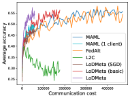
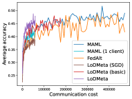
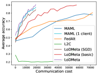
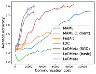
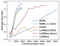
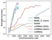
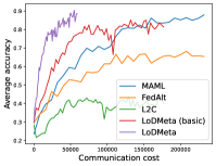
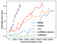
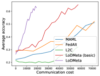
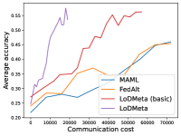
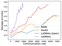
Mini-ImageNet. Figure 1 compares the testing accuracies of training clients with communication cost for different methods. We use the relative communication cost as in Table 1. Among random-walk methods, while LoDMeta(SGD) performs a bit worse, LoDMeta(basic) and LoDMeta achieve comparable performances with the centralized learning methods (MAML and FedAlt), and do not need additional central server to coordinate the learning process. This agrees with Theorem 4.3, which shows Algorithm 2 has the same asymptotic convergence rate as centralized methods. It also demonstrates the necessity of using adaptive optimizers for meta-learning problems. Moreover, L2C has worse performance than reported in Li et al. (2022a). This may be due to that we use fewer training samples and smaller number of neighbors, and L2C overfits.²²2For the mini-ImageNet experiment, Li et al. (2022a) use 500 samples for each client (50 samples per class), and each client has 10 neighbors. Here, we use 100 samples for each client (20 samples per class), and the maximum number of neighbors is 5. LoDMeta is also more preferable than LoDMeta(basic) in the decentralized setting due to its smaller communication cost.

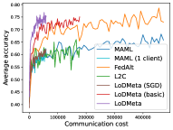
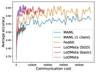
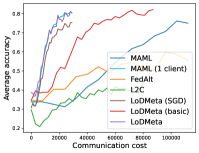
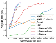
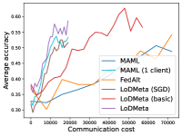
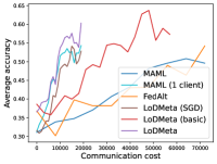
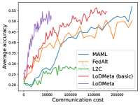
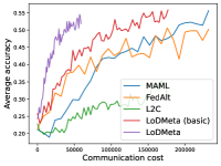
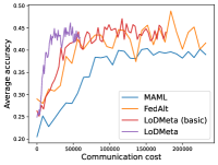
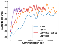
Figure 2 compares the testing accuracy of unseen clients with communication cost for different methods and communication networks. L2C is not compared on the unseen clients as it can only produce models for the training clients. Similar to the testing accuracies for training clients, LoDMeta (basic) and LoDMeta both achieve comparable or even better performance than the centralized learning methods (MAML and FedAlt), and LoDMeta has significantly smaller communication cost compared with LoDMeta (basic).

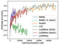
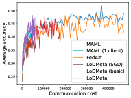
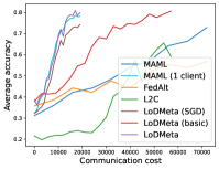
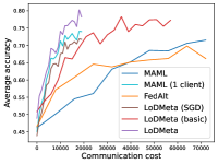
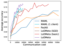
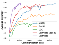
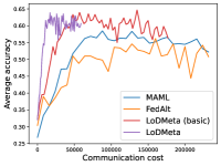
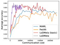
Meta-Datasets. Figure 3 compares the testing accuracies of training clients with communication cost for different methods and communication networks. Within limited communication resources, LoDMeta achieves the best performances, which comes from its significantly smaller per-iteration communication cost (1/3 of L2C/LoDMeta(basic) as in Table 1). Among all the baseline methods, L2C still has poorer performances than both centralized methods (MAML and FedAlt) and random-walk methods (LoDMeta(SGD), LoDMeta(basic) and LoDMeta).

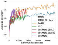
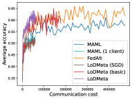
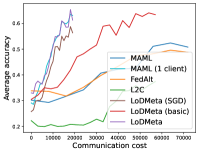
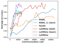
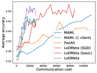
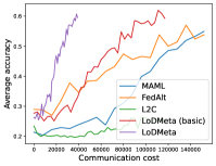
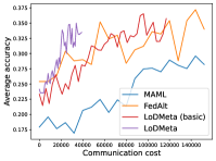
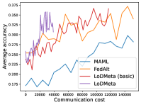
Figure 4 compares the testing accuracy of unseen clients with communication cost for different methods and communication networks. LoDMeta(basic) and LoDMeta achieve much better performances than the centralized learning methods (MAML and FedAlt). Compared with LoDMeta(basic), LoDMeta further reduces the communication cost, and achieves the best performance.

Effect of Random Perturbations for Privacy. Since there are limited works on privacy protection for decentralized meta-learning, here we study the performance of LoDMeta at different amounts of privacy perturbation, which is controlled by the two hyper-parameters $\epsilon,\delta$ used to generate the random perturbation $\bm{\epsilon}_{t}$ . Table 2 (resp. Table 3) compares the testing accuracies on training (resp. unseen) clients with different $\epsilon$ and $\delta$ ’s in Algorithm 2. As is shown in Theorem 4.5, a larger perturbation (which corresponds to a smaller $\epsilon$ or $\delta$ ) leads to better privacy protection. From both Tables 2 and 3, a smaller $\epsilon$ or $\delta$ leads to worse testing accuracies. Hence, there is a trade-off between privacy protection and model performance, which agrees with studies on other settings Hu et al. (2020); Cyffers and Bellet (2022).

6 Conclusion

In this paper, we proposed a novel random-walk-based decentralized meta-learning algorithm (LoDMeta) in which the learning clients perform different tasks with limited data. It uses local auxiliary parameters to remove the communication overhead associated with adaptive optimizers. To better protect data privacy for each client, LoDMeta also introduces random perturbations to the model parameter. Theoretical analysis demonstrates that LoDMeta achieves the same convergence rate as centralized meta-learning algorithms. Empirical few-shot learning results demonstrate that LoDMeta has similar accuracy as centralized meta-learning algorithms, but does not require gathering data from each client and is able to protect data privacy for each client.

References

Balcan et al. (2012) Maria Florina Balcan, Avrim Blum, Shai Fine, and Yishay Mansour. Distributed learning, communication complexity and privacy. In Conference on Learning Theory, 2012.
Bertsekas (1997) Dimitris P. Bertsekas. A new class of incremental gradient methods for least squares problems. SIAM Journal on Optimization, 7(4):913–926, 1997.
Boyd et al. (2011) Stephen Boyd, Neal Parikh, Eric Chu, Borja Peleato, and Jonathan Eckstein. Distributed optimization and statistical learning via the alternating direction method of multipliers. Foundations and Trends® in Machine learning, 3(1):1–122, 2011.
Chen et al. (2023) Xuxing Chen, Minhui Huang, Shiqian Ma, and Krishna Balasubramanian. Decentralized stochastic bilevel optimization with improved per-iteration complexity. In Proceedings of the 40th International Conference on Machine Learning, pages 4641–4671, 2023.
Collins et al. (2021) Liam Collins, Hamed Hassani, Aryan Mokhtari, and Sanjay Shakkottai. Exploiting Shared Representations for Personalized Federated Learning. In International Conference on Machine Learning, 2021.
Cyffers and Bellet (2022) Edwige Cyffers and Aurélien Bellet. Privacy amplification by decentralization. In International Conference on Artificial Intelligence and Statistics, 2022.
Cyffers et al. (2022) Edwige Cyffers, Mathieu Even, Aurélien Bellet, and Laurent Massoulié. Muffliato: Peer-to-peer privacy amplification for decentralized optimization and averaging. Neural Information Processing Systems, 2022.
Duchi et al. (2011) John Duchi, Elad Hazan, and Yoram Singer. Adaptive subgradient methods for online learning and stochastic optimization. In Journal of machine learning research, volume 12, pages 2121–2159, 2011.
Dwork et al. (2014) Cynthia Dwork, Aaron Roth, et al. The algorithmic foundations of differential privacy. Foundations and Trends® in Theoretical Computer Science, 9(3–4):211–407, 2014.
Fallah et al. (2020a) Alireza Fallah, Aryan Mokhtari, and Asuman Ozdaglar. On the convergence theory of gradient-based model-agnostic meta-learning algorithms. In International Conference on Artificial Intelligence and Statistics, 2020a.
Fallah et al. (2020b) Alireza Fallah, Aryan Mokhtari, and Asuman Ozdaglar. On the convergence theory of gradient-based model-agnostic meta-learning algorithms. In Proceedings of the 23rd International Conference on Artificial Intelligence and Statistics, pages 1082–1092, 2020b.
Feldman et al. (2018) Vitaly Feldman, Ilya Mironov, Kunal Talwar, and Abhradeep Thakurta. Privacy amplification by iteration. In 2018 IEEE 59th Annual Symposium on Foundations of Computer Science, 2018.
Finn et al. (2017) Chelsea Finn, Pieter Abbeel, and Sergey Levine. Model-agnostic meta-learning for fast adaptation of deep networks. In International Conference on Machine Learning, 2017.
Flennerhag et al. (2022) Sebastian Flennerhag, Yannick Schroecker, Tom Zahavy, Hado van Hasselt, David Silver, and Satinder Singh. Bootstrapped Meta-Learning. In International Conference on Learning Representations, 2022.
Hospedales et al. (2022) Timothy Hospedales, Antreas Antoniou, Paul Micaelli, and Amos Storkey. Meta-learning in neural networks: A survey. IEEE Transactions on Pattern Analysis and Machine Intelligence, 44(9):5149–5169, 2022.
Hu et al. (2020) Rui Hu, Yuanxiong Guo, Hongning Li, Qingqi Pei, and Yanmin Gong. Personalized federated learning with differential privacy. IEEE Internet of Things Journal, 7(10):9530–9539, 2020.
Ji et al. (2020) Kaiyi Ji, Junjie Yang, and Yingbin Liang. Theoretical Convergence of Multi-Step Model-Agnostic Meta-Learning. Technical Report arXiv:2002.07836, 2020.
Johansson et al. (2010) Björn Johansson, Maben Rabi, and Mikael Johansson. A randomized incremental subgradient method for distributed optimization in networked systems. SIAM Journal on Optimization, 20(3):1157–1170, 2010.
Kayaalp et al. (2020) Mert Kayaalp, Stefan Vlaski, and Ali H. Sayed. Dif-maml: Decentralized multi-agent meta-learning. IEEE Open Journal of Signal Processing, 3:71–93, 2020.
Koloskova et al. (2020) Anastasia Koloskova, Nicolas Loizou, Sadra Boreiri, Martin Jaggi, and Sebastian Stich. A Unified Theory of Decentralized SGD with Changing Topology and Local Updates. In International Conference on Machine Learning, 2020.
Li et al. (2022a) Shuangtong Li, Tianyi Zhou, Xinmei Tian, and Dacheng Tao. Learning to collaborate in decentralized learning of personalized models. In IEEE/CVF Conference on Computer Vision and Pattern Recognition, 2022a.
Li et al. (2022b) Tian Li, Manzil Zaheer, Sashank Reddi, and Virginia Smith. Private adaptive optimization with side information. In International Conference on Machine Learning, 2022b.
Li et al. (2023) Tian Li, Manzil Zaheer, Ken Liu, Sashank J Reddi, Hugh Brendan McMahan, and Virginia Smith. Differentially private adaptive optimization with delayed preconditioners. In International Conference on Learning Representations, 2023.
Liu et al. (2023) Zhuqing Liu, Xin Zhang, Prashant Khanduri, Songtao Lu, and Jia Liu. Prometheus: Taming sample and communication complexities in constrained decentralized stochastic bilevel learning. In Proceedings of the 40th International Conference on Machine Learning, pages 22420–22453, 2023.
Lu and De Sa (2021) Yucheng Lu and Christopher De Sa. Optimal Complexity in Decentralized Training. In International Conference on Machine Learning, 2021.
Mao et al. (2019) Xianghui Mao, Yuantao Gu, and Wotao Yin. Walk Proximal Gradient: An Energy-Efficient Algorithm for Consensus Optimization. IEEE Internet of Things Journal, 6(2):2048–2060, 2019.
Mao et al. (2020) Xianghui Mao, Kun Yuan, Yubin Hu, Yuantao Gu, Ali H. Sayed, and Wotao Yin. Walkman: A Communication-Efficient Random-Walk Algorithm for Decentralized Optimization. IEEE Transactions on Signal Processing, 68:2513–2528, 2020.
Marfoq et al. (2022) Othmane Marfoq, Giovanni Neglia, Richard Vidal, and Laetitia Kameni. Personalized Federated Learning through Local Memorization. In International Conference on Machine Learning, 2022.
McMahan et al. (2017) Brendan McMahan, Eider Moore, Daniel Ramage, Seth Hampson, and Blaise Aguera y Arcas. Communication-efficient learning of deep networks from decentralized data. In International Conference on Artificial Intelligence and Statistics, 2017.
McMahan et al. (2018) H Brendan McMahan, Daniel Ramage, Kunal Talwar, and Li Zhang. Learning differentially private recurrent language models. In International Conference on Learning Representations, 2018.
Mironov (2017) Ilya Mironov. Rényi differential privacy. In IEEE 30th Computer Security Foundations Symposium, 2017.
Nichol et al. (2018) Alex Nichol, Joshua Achiam, and John Schulman. On First-Order Meta-Learning Algorithms. Technical Report arXiv:1803.02999, 2018.
Pillutla et al. (2022) Krishna Pillutla, Kshitiz Malik, Abdel-Rahman Mohamed, Mike Rabbat, Maziar Sanjabi, and Lin Xiao. Federated Learning with Partial Model Personalization. In International Conference on Machine Learning, 2022.
Predd et al. (2009) Joel B Predd, Sanjeev R Kulkarni, and H Vincent Poor. A collaborative training algorithm for distributed learning. IEEE Transactions on Information Theory, 55(4):1856–1871, 2009.
Raghu et al. (2020) Aniruddh Raghu, Maithra Raghu, Samy Bengio, and Oriol Vinyals. Rapid learning or feature reuse? Towards understanding the effectiveness of MAML. In International Conference on Learning Representations, 2020.
Ravi and Larochelle (2017) Sachin Ravi and Hugo Larochelle. Optimization as a model for few-shot learning. In International Conference on Learning Representations, 2017.
Rényi (1961) Alfréd Rényi. On measures of entropy and information. In Proceedings of the Fourth Berkeley Symposium on Mathematical Statistics and Probability, Volume 1: Contributions to the Theory of Statistics, 1961.
Shu et al. (2019) Jun Shu, Qi Xie, Lixuan Yi, Qian Zhao, Sanping Zhou, Zongben Xu, and Deyu Meng. Meta-weight-net: Learning an explicit mapping for sample weighting. In Neural Information Processing Systems, 2019.
Singhal et al. (2021) Karan Singhal, Hakim Sidahmed, Zachary Garrett, Shanshan Wu, John Rush, and Sushant Prakash. Federated Reconstruction: Partially Local Federated Learning. In Neural Information Processing Systems, 2021.
Sun et al. (2022) Tao Sun, Dongsheng Li, and Bao Wang. Adaptive Random Walk Gradient Descent for Decentralized Optimization. In International Conference on Machine Learning, 2022.
Triantafillou et al. (2020) Eleni Triantafillou, Tyler Zhu, Vincent Dumoulin, Pascal Lamblin, Utku Evci, Kelvin Xu, Ross Goroshin, Carles Gelada, Kevin Swersky, Pierre-Antoine Manzagol, and Hugo Larochelle. Meta-dataset: A dataset of datasets for learning to learn from few examples. In International Conference on Learning Representations, 2020.
Triastcyn et al. (2022) Aleksei Triastcyn, Matthias Reisser, and Christos Louizos. Decentralized Learning with Random Walks and Communication-Efficient Adaptive Optimization. In Workshop on Federated Learning: Recent Advances and New Challenges (in Conjunction with NeurIPS 2022), 2022. URL https://openreview.net/forum?id=QwL8ZGl_QGG.
Watts and Strogatz (1998) Duncan J Watts and Steven H Strogatz. Collective dynamics of ‘small-world’networks. Nature, 393(6684):440–442, 1998.
Wei et al. (2020) Kang Wei, Jun Li, Ming Ding, Chuan Ma, Howard H Yang, Farhad Farokhi, Shi Jin, Tony QS Quek, and H Vincent Poor. Federated learning with differential privacy: Algorithms and performance analysis. IEEE Transactions on Information Forensics and Security, 15:3454–3469, 2020.
Xie et al. (2022) Zeke Xie, Xinrui Wang, Huishuai Zhang, Issei Sato, and Masashi Sugiyama. Adaptive inertia: Disentangling the effects of adaptive learning rate and momentum. In Proceedings of the 39th International Conference on Machine Learning, pages 24430–24459, 2022.
Yang and Kwok (2022) Hansi Yang and James Kwok. Efficient variance reduction for meta-learning. In Proceedings of the 39th International Conference on Machine Learning, pages 25070–25095, 2022.
Yang et al. (2022) Shuoguang Yang, Xuezhou Zhang, and Mengdi Wang. Decentralized gossip-based stochastic bilevel optimization over communication networks. In Advances in Neural Information Processing Systems, volume 35, pages 238–252, 2022.
Yang et al. (2023) Yifan Yang, Peiyao Xiao, and Kaiyi Ji. Simfbo: Towards simple, flexible and communication-efficient federated bilevel learning. In Advances in Neural Information Processing Systems, volume 36, pages 33027–33040, 2023.
Yao et al. (2019) Huaxiu Yao, Ying Wei, Junzhou Huang, and Zhenhui Li. Hierarchically structured meta-learning. In International Conference on Machine Learning, 2019.
Yuan et al. (2022) Binhang Yuan, Yongjun He, Jared Quincy Davis, Tianyi Zhang, Tri Dao, Beidi Chen, Percy Liang, Christopher Re, and Ce Zhang. Decentralized training of foundation models in heterogeneous environments. In Neural Information Processing Systems, 2022.
Yuan et al. (2021) Kun Yuan, Yiming Chen, Xinmeng Huang, Yingya Zhang, Pan Pan, Yinghui Xu, and Wotao Yin. DecentLaM: Decentralized Momentum SGD for Large-Batch Deep Training. In IEEE/CVF International Conference on Computer Vision, 2021.
Zhang et al. (2022) Xianyang Zhang, Chen Hu, Bing He, and Zhiguo Han. Distributed reptile algorithm for meta-learning over multi-agent systems. IEEE Transactions on Signal Processing, 70:5443–5456, 2022.
Zhou and Bassily (2022) Xinyu Zhou and Raef Bassily. Task-level differentially private meta learning. In Neural Information Processing Systems, 2022.
Zhuang et al. (2020) Juntang Zhuang, Tommy Tang, Yifan Ding, Sekhar C Tatikonda, Nicha Dvornek, Xenophon Papademetris, and James Duncan. Adabelief optimizer: Adapting stepsizes by the belief in observed gradients. Advances in neural information processing systems, 33:18795–18806, 2020.

NeurIPS Paper Checklist

1.

Claims
Question: Do the main claims made in the abstract and introduction accurately reflect the paper’s contributions and scope?
Answer: [Yes]
Justification: the claims made in abstract and introduction (section 1) clearly reflects the paper’s contributions and scope.
Guidelines:
- •
  
  The answer NA means that the abstract and introduction do not include the claims made in the paper.
- •
  
  The abstract and/or introduction should clearly state the claims made, including the contributions made in the paper and important assumptions and limitations. A No or NA answer to this question will not be perceived well by the reviewers.
- •
  
  The claims made should match theoretical and experimental results, and reflect how much the results can be expected to generalize to other settings.
- •
  
  It is fine to include aspirational goals as motivation as long as it is clear that these goals are not attained by the paper.
2.

Limitations
Question: Does the paper discuss the limitations of the work performed by the authors?
Answer: [Yes]
Justification: we have discussed possible limitations in in Appendix A.
Guidelines:
- •
  
  The answer NA means that the paper has no limitation while the answer No means that the paper has limitations, but those are not discussed in the paper.
- •
  
  The authors are encouraged to create a separate "Limitations" section in their paper.
- •
  
  The paper should point out any strong assumptions and how robust the results are to violations of these assumptions (e.g., independence assumptions, noiseless settings, model well-specification, asymptotic approximations only holding locally). The authors should reflect on how these assumptions might be violated in practice and what the implications would be.
- •
  
  The authors should reflect on the scope of the claims made, e.g., if the approach was only tested on a few datasets or with a few runs. In general, empirical results often depend on implicit assumptions, which should be articulated.
- •
  
  The authors should reflect on the factors that influence the performance of the approach. For example, a facial recognition algorithm may perform poorly when image resolution is low or images are taken in low lighting. Or a speech-to-text system might not be used reliably to provide closed captions for online lectures because it fails to handle technical jargon.
- •
  
  The authors should discuss the computational efficiency of the proposed algorithms and how they scale with dataset size.
- •
  
  If applicable, the authors should discuss possible limitations of their approach to address problems of privacy and fairness.
- •
  
  While the authors might fear that complete honesty about limitations might be used by reviewers as grounds for rejection, a worse outcome might be that reviewers discover limitations that aren’t acknowledged in the paper. The authors should use their best judgment and recognize that individual actions in favor of transparency play an important role in developing norms that preserve the integrity of the community. Reviewers will be specifically instructed to not penalize honesty concerning limitations.
3.

Theory Assumptions and Proofs
Question: For each theoretical result, does the paper provide the full set of assumptions and a complete (and correct) proof?
Answer: [Yes]
Justification: the assumptions are all mentioned in section 4, and all proofs can be found in Appendix E.
Guidelines:
- •
  
  The answer NA means that the paper does not include theoretical results.
- •
  
  All the theorems, formulas, and proofs in the paper should be numbered and cross-referenced.
- •
  
  All assumptions should be clearly stated or referenced in the statement of any theorems.
- •
  
  The proofs can either appear in the main paper or the supplemental material, but if they appear in the supplemental material, the authors are encouraged to provide a short proof sketch to provide intuition.
- •
  
  Inversely, any informal proof provided in the core of the paper should be complemented by formal proofs provided in appendix or supplemental material.
- •
  
  Theorems and Lemmas that the proof relies upon should be properly referenced.
4.

Experimental Result Reproducibility
Question: Does the paper fully disclose all the information needed to reproduce the main experimental results of the paper to the extent that it affects the main claims and/or conclusions of the paper (regardless of whether the code and data are provided or not)?
Answer: [Yes]
Justification: we have mentioned necessary experimental settings in Appendix C to reproduce our experimental results.
Guidelines:
- •
  
  The answer NA means that the paper does not include experiments.
- •
  
  If the paper includes experiments, a No answer to this question will not be perceived well by the reviewers: Making the paper reproducible is important, regardless of whether the code and data are provided or not.
- •
  
  If the contribution is a dataset and/or model, the authors should describe the steps taken to make their results reproducible or verifiable.
- •
  
  Depending on the contribution, reproducibility can be accomplished in various ways. For example, if the contribution is a novel architecture, describing the architecture fully might suffice, or if the contribution is a specific model and empirical evaluation, it may be necessary to either make it possible for others to replicate the model with the same dataset, or provide access to the model. In general. releasing code and data is often one good way to accomplish this, but reproducibility can also be provided via detailed instructions for how to replicate the results, access to a hosted model (e.g., in the case of a large language model), releasing of a model checkpoint, or other means that are appropriate to the research performed.
- •
  While NeurIPS does not require releasing code, the conference does require all submissions to provide some reasonable avenue for reproducibility, which may depend on the nature of the contribution. For example
  1. (a)
    
    If the contribution is primarily a new algorithm, the paper should make it clear how to reproduce that algorithm.
  2. (b)
    
    If the contribution is primarily a new model architecture, the paper should describe the architecture clearly and fully.
  3. (c)
    
    If the contribution is a new model (e.g., a large language model), then there should either be a way to access this model for reproducing the results or a way to reproduce the model (e.g., with an open-source dataset or instructions for how to construct the dataset).
  4. (d)
    
    We recognize that reproducibility may be tricky in some cases, in which case authors are welcome to describe the particular way they provide for reproducibility. In the case of closed-source models, it may be that access to the model is limited in some way (e.g., to registered users), but it should be possible for other researchers to have some path to reproducing or verifying the results.
5.

Open access to data and code
Question: Does the paper provide open access to the data and code, with sufficient instructions to faithfully reproduce the main experimental results, as described in supplemental material?
Answer: [No]
Justification: since our code also includes scripts from other open-source packages, it takes more time to arrange our code. We will release our code along with camera-ready version if our submission is accepted.
Guidelines:
- •
  
  The answer NA means that paper does not include experiments requiring code.
- •
  
  Please see the NeurIPS code and data submission guidelines (https://nips.cc/public/guides/CodeSubmissionPolicy) for more details.
- •
  
  While we encourage the release of code and data, we understand that this might not be possible, so “No” is an acceptable answer. Papers cannot be rejected simply for not including code, unless this is central to the contribution (e.g., for a new open-source benchmark).
- •
  
  The instructions should contain the exact command and environment needed to run to reproduce the results. See the NeurIPS code and data submission guidelines (https://nips.cc/public/guides/CodeSubmissionPolicy) for more details.
- •
  
  The authors should provide instructions on data access and preparation, including how to access the raw data, preprocessed data, intermediate data, and generated data, etc.
- •
  
  The authors should provide scripts to reproduce all experimental results for the new proposed method and baselines. If only a subset of experiments are reproducible, they should state which ones are omitted from the script and why.
- •
  
  At submission time, to preserve anonymity, the authors should release anonymized versions (if applicable).
- •
  
  Providing as much information as possible in supplemental material (appended to the paper) is recommended, but including URLs to data and code is permitted.
6.

Experimental Setting/Details
Question: Does the paper specify all the training and test details (e.g., data splits, hyperparameters, how they were chosen, type of optimizer, etc.) necessary to understand the results?
Answer: [Yes]
Justification: we have mentioned necessary experimental settings (including data splits, hyper-parameters and how they were chosen, type of optimizer) in Appendix C.
Guidelines:
- •
  
  The answer NA means that the paper does not include experiments.
- •
  
  The experimental setting should be presented in the core of the paper to a level of detail that is necessary to appreciate the results and make sense of them.
- •
  
  The full details can be provided either with the code, in appendix, or as supplemental material.
7.

Experiment Statistical Significance
Question: Does the paper report error bars suitably and correctly defined or other appropriate information about the statistical significance of the experiments?
Answer: [No]
Justification: we do not report error bars in our experimental results.
Guidelines:
- •
  
  The answer NA means that the paper does not include experiments.
- •
  
  The authors should answer "Yes" if the results are accompanied by error bars, confidence intervals, or statistical significance tests, at least for the experiments that support the main claims of the paper.
- •
  
  The factors of variability that the error bars are capturing should be clearly stated (for example, train/test split, initialization, random drawing of some parameter, or overall run with given experimental conditions).
- •
  
  The method for calculating the error bars should be explained (closed form formula, call to a library function, bootstrap, etc.)
- •
  
  The assumptions made should be given (e.g., Normally distributed errors).
- •
  
  It should be clear whether the error bar is the standard deviation or the standard error of the mean.
- •
  
  It is OK to report 1-sigma error bars, but one should state it. The authors should preferably report a 2-sigma error bar than state that they have a 96% CI, if the hypothesis of Normality of errors is not verified.
- •
  
  For asymmetric distributions, the authors should be careful not to show in tables or figures symmetric error bars that would yield results that are out of range (e.g. negative error rates).
- •
  
  If error bars are reported in tables or plots, The authors should explain in the text how they were calculated and reference the corresponding figures or tables in the text.
8.

Experiments Compute Resources
Question: For each experiment, does the paper provide sufficient information on the computer resources (type of compute workers, memory, time of execution) needed to reproduce the experiments?
Answer: [Yes]
Justification: we mentioned compute resources used in our experiments in Appendix C.
Guidelines:
- •
  
  The answer NA means that the paper does not include experiments.
- •
  
  The paper should indicate the type of compute workers CPU or GPU, internal cluster, or cloud provider, including relevant memory and storage.
- •
  
  The paper should provide the amount of compute required for each of the individual experimental runs as well as estimate the total compute.
- •
  
  The paper should disclose whether the full research project required more compute than the experiments reported in the paper (e.g., preliminary or failed experiments that didn’t make it into the paper).
9.

Code Of Ethics
Question: Does the research conducted in the paper conform, in every respect, with the NeurIPS Code of Ethics https://neurips.cc/public/EthicsGuidelines?
Answer: [Yes]
Justification: we have thoroughly checked the code of ethics and found no conflict.
Guidelines:
- •
  
  The answer NA means that the authors have not reviewed the NeurIPS Code of Ethics.
- •
  
  If the authors answer No, they should explain the special circumstances that require a deviation from the Code of Ethics.
- •
  
  The authors should make sure to preserve anonymity (e.g., if there is a special consideration due to laws or regulations in their jurisdiction).
10.

Broader Impacts
Question: Does the paper discuss both potential positive societal impacts and negative societal impacts of the work performed?
Answer: [Yes]
Justification: we have discussed possible societal impacts of our proposed method in Appendix A.
Guidelines:
- •
  
  The answer NA means that there is no societal impact of the work performed.
- •
  
  If the authors answer NA or No, they should explain why their work has no societal impact or why the paper does not address societal impact.
- •
  
  Examples of negative societal impacts include potential malicious or unintended uses (e.g., disinformation, generating fake profiles, surveillance), fairness considerations (e.g., deployment of technologies that could make decisions that unfairly impact specific groups), privacy considerations, and security considerations.
- •
  
  The conference expects that many papers will be foundational research and not tied to particular applications, let alone deployments. However, if there is a direct path to any negative applications, the authors should point it out. For example, it is legitimate to point out that an improvement in the quality of generative models could be used to generate deepfakes for disinformation. On the other hand, it is not needed to point out that a generic algorithm for optimizing neural networks could enable people to train models that generate Deepfakes faster.
- •
  
  The authors should consider possible harms that could arise when the technology is being used as intended and functioning correctly, harms that could arise when the technology is being used as intended but gives incorrect results, and harms following from (intentional or unintentional) misuse of the technology.
- •
  
  If there are negative societal impacts, the authors could also discuss possible mitigation strategies (e.g., gated release of models, providing defenses in addition to attacks, mechanisms for monitoring misuse, mechanisms to monitor how a system learns from feedback over time, improving the efficiency and accessibility of ML).
11.

Safeguards
Question: Does the paper describe safeguards that have been put in place for responsible release of data or models that have a high risk for misuse (e.g., pretrained language models, image generators, or scraped datasets)?
Answer: [N/A]
Justification: this paper does not involve releasing any data or models that may have risk for misuse.
Guidelines:
- •
  
  The answer NA means that the paper poses no such risks.
- •
  
  Released models that have a high risk for misuse or dual-use should be released with necessary safeguards to allow for controlled use of the model, for example by requiring that users adhere to usage guidelines or restrictions to access the model or implementing safety filters.
- •
  
  Datasets that have been scraped from the Internet could pose safety risks. The authors should describe how they avoided releasing unsafe images.
- •
  
  We recognize that providing effective safeguards is challenging, and many papers do not require this, but we encourage authors to take this into account and make a best faith effort.
12.

Licenses for existing assets
Question: Are the creators or original owners of assets (e.g., code, data, models), used in the paper, properly credited and are the license and terms of use explicitly mentioned and properly respected?
Answer: [Yes]
Justification: we mentioned licenses for data sets used in our work in Appendix C.
Guidelines:
- •
  
  The answer NA means that the paper does not use existing assets.
- •
  
  The authors should cite the original paper that produced the code package or dataset.
- •
  
  The authors should state which version of the asset is used and, if possible, include a URL.
- •
  
  The name of the license (e.g., CC-BY 4.0) should be included for each asset.
- •
  
  For scraped data from a particular source (e.g., website), the copyright and terms of service of that source should be provided.
- •
  
  If assets are released, the license, copyright information, and terms of use in the package should be provided. For popular datasets, paperswithcode.com/datasets has curated licenses for some datasets. Their licensing guide can help determine the license of a dataset.
- •
  
  For existing datasets that are re-packaged, both the original license and the license of the derived asset (if it has changed) should be provided.
- •
  
  If this information is not available online, the authors are encouraged to reach out to the asset’s creators.
13.

New Assets
Question: Are new assets introduced in the paper well documented and is the documentation provided alongside the assets?
Answer: [N/A]
Justification: this paper does not release any new assets.
Guidelines:
- •
  
  The answer NA means that the paper does not release new assets.
- •
  
  Researchers should communicate the details of the dataset/code/model as part of their submissions via structured templates. This includes details about training, license, limitations, etc.
- •
  
  The paper should discuss whether and how consent was obtained from people whose asset is used.
- •
  
  At submission time, remember to anonymize your assets (if applicable). You can either create an anonymized URL or include an anonymized zip file.
14.

Crowdsourcing and Research with Human Subjects
Question: For crowdsourcing experiments and research with human subjects, does the paper include the full text of instructions given to participants and screenshots, if applicable, as well as details about compensation (if any)?
Answer: [N/A]
Justification: this paper does not involve crowdsourcing nor research with human subjects.
Guidelines:
- •
  
  The answer NA means that the paper does not involve crowdsourcing nor research with human subjects.
- •
  
  Including this information in the supplemental material is fine, but if the main contribution of the paper involves human subjects, then as much detail as possible should be included in the main paper.
- •
  
  According to the NeurIPS Code of Ethics, workers involved in data collection, curation, or other labor should be paid at least the minimum wage in the country of the data collector.
15.

Institutional Review Board (IRB) Approvals or Equivalent for Research with Human Subjects
Question: Does the paper describe potential risks incurred by study participants, whether such risks were disclosed to the subjects, and whether Institutional Review Board (IRB) approvals (or an equivalent approval/review based on the requirements of your country or institution) were obtained?
Answer: [N/A]
Justification: this paper does not involve crowdsourcing nor research with human subjects.
Guidelines:
- •
  
  The answer NA means that the paper does not involve crowdsourcing nor research with human subjects.
- •
  
  Depending on the country in which research is conducted, IRB approval (or equivalent) may be required for any human subjects research. If you obtained IRB approval, you should clearly state this in the paper.
- •
  
  We recognize that the procedures for this may vary significantly between institutions and locations, and we expect authors to adhere to the NeurIPS Code of Ethics and the guidelines for their institution.
- •
  
  For initial submissions, do not include any information that would break anonymity (if applicable), such as the institution conducting the review.

Appendix A Possible Limitations and Broader Impacts

Limitations. One possible limitation of this work is that we only consider network DP for privacy protection. We will consider other privacy metric as future works.

Broader Impacts. As a paper on pure machine learning algorithms, there should be no direct societal impact of this work. Our proposed algorithm is not about generative models and there is no concern on generating fake contents.

Appendix B Algorithms

Algorithm 3 Model adaptation on unseen clients.

1: Input: meta-trained model

{\bm{w}}_{T}

2: initialize

{\bm{u}}_{0}={\bm{w}}_{T}

3: for

k=0

K-1

4: compute

{\bm{g}}_{k}=\nabla\ell({\bm{u}}_{k};\xi^{s}_{i_{t}})

with support data

\xi^{s}_{i_{t}}

of client

i_{t}

;

5: update

{\bm{u}}_{k+1}={\bm{u}}_{k}-\alpha{\bm{g}}_{k}

;

6: end for

7: obtain the final model

{\bm{u}}_{K}

for testing

Appendix C Details for Experiments

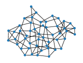
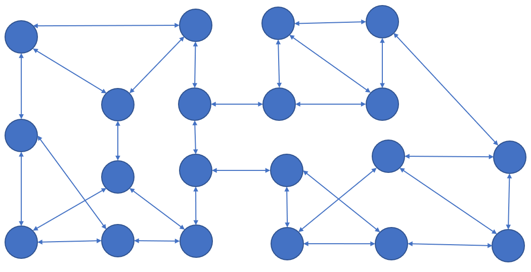
Some statistics for data sets used in experiments are in Table 4. All data sets used in our experiments are released under Apache 2.0 license. Figure 5(a) gives an example for small-world network, while Figure 5(b) gives an example for 3-regular expander network. These two network types are used in our experiments (with different number of clients).

Table 4: Statistics for the data sets used in experiments.

		number of classes			#clients for 1-shot/5-shot setting
		meta-training	meta-testing	#samples per class	training clients	unseen clients
Meta-Dataset	Bird	80	20	60	38/38	12/12
	Texture	37	10	120	42/36	14/12
	Aircraft	80	20	100	76/64	24/20
	Fungi	80	20	150	115/89	36/28
mini-Imagenet		80	20	600	380/380	120/120

All experiments are run on a single RTX2080 Ti GPU. Following [13, 32], we use the CONV4³³3The CONV4 model is a 4-layer CNN. Each layer contains 64 $3\times 3$ convolutional filters, followed by batch normalization, ReLU activation, and $2\times 2$ max-pooling. as base learner. The hyper-parameter settings for all data sets also follow MAML [13]: learning rate $\eta$ is $0.001$ , first-order momentum weight $\theta$ is $0$ , and the second-order momentum weight $\beta$ is $0.99$ . The number of gradient descent steps ( $K$ ) in the inner loop is 5. Unless otherwise specified, we set $\epsilon=0.5$ and $\delta=0.3$ for the privacy perturbation.

Appendix D Additional Experimental Results

D.1 Experiments on 1-shot Meta-Datasets with small-world network

Figure 6 compares the average testing accuracy across different clients during training on these four data sets under the 1-shot setting with the number of training iterations. Similar to the 5-shot learning setting, the two random-walk algorithms (DMAML and LDMeta) achieve slightly worse performance than MAML, but better performance than FedAlt. Compared to the 5-shot setting (Figure 7), the gossip-based algorithm L2C performs even worse in this 1-shot setting because each client has even fewer samples.

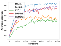
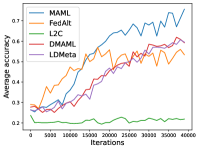
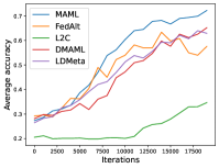
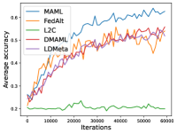
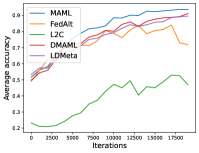
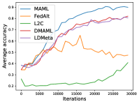
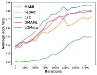
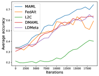
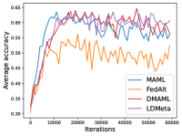
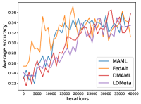
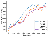
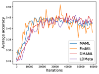
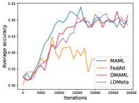
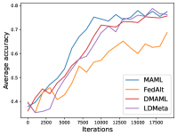
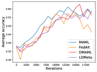
Figure 8 compares the average testing accuracy across different clients during training on these four data sets under the 1-shot setting with communication cost. Similar to the 5-shot learning setting (Figure 3), LDMeta has a much smaller communication cost than DMAML, and is more preferable when we require communication to be efficient.

D.2 Experiments with 3-regular network

Here, we perform experiments on the 3-regular expander graph, in which all clients have 3 neighbors. The other settings are the same as experiments in the main text.

Figure 9 compares the average testing accuracy across different clients during training on four data sets in Meta-Datasets with the number of training iterations. As can be seen, the two random-walk algorithms (DMAML and LDMeta) have slightly worse performance than MAML, but better performance than FedAlt, and significantly outperform the gossip-based algorithm L2C. This is because in the random-walk setting, only one client needs to update the meta-model in each iteration, while personalized federated learning methods require multiple clients to update the meta-model.

Appendix E Proofs

E.1 Proof of Proposition 4.2

By the definition of $G_{i}(\cdot)$ , we have

$\displaystyle\\|G_{i}({\bm{w}})-G_{i}({\bm{u}})\\|\leq$	$\displaystyle\Big{\\|}\prod_{k=0}^{K-1}({\bm{I}}-\alpha\nabla^{2}\ell({\bm{w}}_{k};\xi^{s}_{i}))\nabla\ell({\bm{w}}_{K};\xi^{q}_{i})-\prod_{k=0}^{K-1}({\bm{I}}-\alpha\nabla^{2}\ell({\bm{u}}_{k};\xi^{s}_{i}))\nabla\ell({\bm{w}}_{K};\xi^{q}_{i})\Big{\\|}$
	$\displaystyle+\Big{\\|}\prod_{k=0}^{K-1}({\bm{I}}-\alpha\nabla^{2}\ell({\bm{u}}_{k};\xi^{s}_{i}))\nabla\ell({\bm{w}}_{K};\xi^{q}_{i})-\prod_{k=0}^{K-1}({\bm{I}}-\alpha\nabla^{2}\ell({\bm{u}}_{k};\xi^{s}_{i}))\nabla\ell({\bm{u}}_{K};\xi^{q}_{i})\Big{\\|}$
$\displaystyle\leq$	$\displaystyle\underbrace{\Big{\\|}\prod_{k=0}^{K-1}({\bm{I}}-\alpha\nabla^{2}\ell({\bm{w}}_{k};\xi^{s}_{i}))-\prod_{k=0}^{K-1}({\bm{I}}-\alpha\nabla^{2}\ell({\bm{u}}_{k};\xi^{s}_{i}))\Big{\\|}}_{A}\\|\nabla\ell({\bm{w}}_{K};\xi^{q}_{i})\\|$
	$\displaystyle+(1+\alpha M)^{K}\\|\nabla\ell({\bm{w}}_{K};\xi^{q}_{i})-\nabla\ell({\bm{u}}_{K};\xi^{q}_{i})\\|.$	(4)

We next upper-bound $A$ in the above inequality. Specifically, we have

$\displaystyle A\leq$	$\displaystyle\Big{\\|}\prod_{k=0}^{K-1}({\bm{I}}-\alpha\nabla^{2}\ell({\bm{w}}_{k};\xi^{s}_{i}))-\prod_{k=0}^{K-2}({\bm{I}}-\alpha\nabla^{2}\ell({\bm{w}}_{k};\xi^{s}_{i}))({\bm{I}}-\alpha\nabla^{2}\ell({\bm{u}}_{K-1};\xi^{s}_{i}))\Big{\\|}$
	$\displaystyle+\Big{\\|}\prod_{k=0}^{K-2}({\bm{I}}-\alpha\nabla^{2}\ell({\bm{w}}_{k};\xi^{s}_{i}))({\bm{I}}-\alpha\nabla^{2}\ell({\bm{u}}_{K-1};\xi^{s}_{i}))-\prod_{k=0}^{K-1}({\bm{I}}-\alpha\nabla^{2}\ell({\bm{u}}_{k};\xi^{s}_{i})))\Big{\\|}$
$\displaystyle\leq$	$\displaystyle\Big{(}(1+\alpha M)^{K-1}\alpha\rho+\frac{\rho}{M}(1+\alpha M)^{K}\big{(}(1+\alpha M)^{K-1}-1\big{)}\Big{)}\\|{\bm{w}}-{\bm{u}}\\|,$	(5)

Combining (E.1) and (E.1) yields

\displaystyle\|G_{i}({\bm{w}})-G_{i}({\bm{u}})\|\leq

\displaystyle\big{(}(1+\alpha M)^{K-1}\alpha\rho+\frac{\rho}{M}(1+\alpha M)^{K}\big{(}(1+\alpha M)^{K-1}-1\big{)}\big{)}\|{\bm{w}}-{\bm{u}}\|\|\nabla\ell({\bm{w}}_{K};\xi^{q}_{i})\|+(1+\alpha M)^{K}M\|{\bm{w}}_{K}-{\bm{u}}_{K}\|.

(6)

To upper-bound $\|\nabla\ell({\bm{w}}_{K};\xi^{q}_{i})\|$ in (6), using the mean value theorem, we have

$\displaystyle\\|\nabla\ell({\bm{w}}_{K};\xi^{q}_{i})\\|=$	$\displaystyle\Big{\\|}\nabla\ell({\bm{w}}-\sum_{k=0}^{K-1}\alpha\nabla\ell({\bm{w}}_{k};\xi^{s}_{i});\xi^{q}_{i})\Big{\\|}$
$\displaystyle\leq$	$\displaystyle\\|\nabla\ell({\bm{w}};\xi^{q}_{i})\\|+\alpha M\sum_{k=0}^{K-1}(1+\alpha L)^{k}\big{\\|}\nabla\ell({\bm{w}}_{k};\xi^{s}_{i})\big{\\|}$
$\displaystyle\leq$	$\displaystyle(1+\alpha M)^{K}\\|\nabla\ell({\bm{w}};\xi^{q}_{i})\\|+\big{(}(1+\alpha M)^{K}-1\big{)}b_{i},$	(7)

For $\|{\bm{w}}_{K}-{\bm{u}}_{K}\|$ , we have:

\displaystyle\|{\bm{w}}_{K}-{\bm{u}}_{K}\|\leq(1+\alpha M)^{K}\|{\bm{w}}-{\bm{u}}\|.

(8)

Combining (6), (E.1) and (8) yields

	$\displaystyle\\|G_{i}({\bm{w}})$	$\displaystyle-G_{i}({\bm{u}})\\|$
	$\displaystyle\leq$	$\displaystyle\Big{(}(1+\alpha M)^{K-1}\alpha\rho+\frac{\rho}{M}(1+\alpha M)^{K}\big{(}(1+\alpha M)^{K-1}-1\big{)}\Big{)}(1+\alpha M)^{K}\\|\nabla l_{T_{i}}(w)\\|\\|w-u\\|$
		$\displaystyle+\Big{(}(1+\alpha M)^{K-1}\alpha\rho+\frac{\rho}{M}(1+\alpha M)^{K}\big{(}(1+\alpha M)^{K-1}-1\big{)}\Big{)}\big{(}(1+\alpha M)^{K}-1\big{)}b_{i}\\|w-u\\|$
		$\displaystyle+(1+\alpha M)^{2K}M\\|{\bm{w}}-{\bm{u}}\\|,$

which yields

\displaystyle\|G_{i}({\bm{w}})-G_{i}({\bm{u}})\|\leq\big{(}(1+\alpha M)^{2K}M+C(b+\|\nabla\ell({\bm{w}};\xi^{q}_{i})\|)\big{)}\|{\bm{w}}-{\bm{u}}\|.

Based on the above inequality and Jensen’s inequality, we finish the proof.

E.2 Proof for Theorem 4.3

Despite Proposition 4.2, we also need to upper-bound the expectation of $\mathbb{E}\|G_{i}({\bm{w}})\|^{2}$ , as follows:

Lemma E.1.

Set $\alpha=\frac{1}{8KM}$ . we have for any ${\bm{w}}$ ,

\displaystyle\mathbb{E}\|G_{i}({\bm{w}})\|^{2}\leq A_{\text{squ}_{1}}\|\nabla\mathcal{L}({\bm{w}})\|^{2}+A_{\text{squ}_{2}},

where $A_{\text{squ}_{1}}=\frac{4(1+\alpha M)^{4K}}{(2-(1+\alpha M)^{2K})^{2}},A_{\text{squ}_{2}}=\frac{4(1+\alpha M)^{8K}}{(2-(1+\alpha M)^{2K})^{2}}(\sigma+b)^{2}+2(1+\alpha)^{4K}(\sigma^{2}+\tilde{b}^{2})$ , and $\tilde{b}^{2}=\frac{1}{|{\mathcal{I}}|}\sum_{i\in{\mathcal{I}}}b_{i}^{2}$ .

Proof.

Conditioning on ${\bm{w}}$ , we have

\displaystyle\mathbb{E}\|G_{i}({\bm{w}})\|^{2}=

\displaystyle\mathbb{E}\Big{\|}\prod_{k=0}^{K-1}({\bm{I}}-\alpha\nabla^{2}\ell({\bm{w}}_{k};\xi^{s}_{i}))\nabla\ell({\bm{w}}_{K};\xi^{q}_{i})\Big{\|}^{2}\leq(1+\alpha M)^{2K}\mathbb{E}\|\nabla\ell({\bm{w}}_{K};\xi^{q}_{i})\|^{2},

Using an approach similar to (E.1), we have:

$\displaystyle\mathbb{E}\\|G_{i}({\bm{w}})\\|^{2}\leq$	$\displaystyle(1+\alpha M)^{2K}2(1+\alpha M)^{2K}\mathbb{E}\\|\nabla\ell({\bm{w}}_{K};\xi^{q}_{i})\\|^{2}+2(1+\alpha M)^{2K}\big{(}(1+\alpha M)^{K}-1\big{)}^{2}\mathbb{E}_{i}b_{i}^{2}$
$\displaystyle\leq$	$\displaystyle 2(1+\alpha M)^{4K}(\\|\nabla\mathcal{L}({\bm{w}})\\|^{2}+\sigma^{2})+2(1+\alpha M)^{2K}\big{(}(1+\alpha M)^{K}-1\big{)}^{2}\widetilde{b}$
$\displaystyle\leq$	$\displaystyle 2(1+\alpha M)^{4K}\Big{(}\frac{2}{C_{1}^{2}}\\|\nabla\mathcal{L}({\bm{w}})\\|^{2}+\frac{2C_{2}^{2}}{C_{1}^{2}}+\sigma^{2}\Big{)}+2(1+\alpha M)^{2K}\big{(}(1+\alpha M)^{K}-1\big{)}^{2}\widetilde{b}^{2}$
$\displaystyle\leq$	$\displaystyle\frac{4(1+\alpha M)^{4K}}{C_{1}^{2}}\\|\nabla\mathcal{L}({\bm{w}})\\|^{2}+\frac{4(1+\alpha M)^{4K}C_{2}^{2}}{C_{1}^{2}}+2(1+\alpha M)^{4K}(\sigma^{2}+\widetilde{b}^{2}),$	(9)

Noting that $C_{2}=\big{(}(1+\alpha M)^{2K}-1\big{)}\sigma+(1+\alpha M)^{K}\big{(}(1+\alpha M)^{K}-1\big{)}b<\big{(}(1+\alpha M)^{2K}-1\big{)}(\sigma+b)$ and using the definitions of $A_{\text{squ}_{1}},A_{\text{squ}_{2}}$ , we finish the proof. ∎

Apart from these propositions, we also need some auxiliary lemmas to prove Theorem 4.3. In the sequel, for any vector ${\bm{v}}$ , define $[{\bm{v}}]^{2}$ as the vector whose elements are the squares of elements in ${\bm{v}}$ .

Lemma E.2.

Suppose function $f:[0,+\infty)\to[0,+\infty)$ is a non-increasing function. Then for any sequence $a_{0},\dots,a_{T}\geq 0$ , we have:

\displaystyle\sum_{t=1}^{T}a_{t}\cdot f(a_{0}+\sum_{t=1}^{T}a_{t})\leq\int_{a_{0}}^{\sum_{t=0}^{T}a_{t}}f(x)dx.

Proof.

Let $s_{t}=\sum_{u=0}^{t}a_{u}$ . Since any $a_{t}\geq 0$ for $t=0,\dots,T$ , obviously we have $s_{t-1}\leq s_{t}$ , and $f(s_{0})\geq f(s_{1})\geq\dots\geq f(s_{T})$ . Therefore, we have:

\displaystyle a_{t}\cdot f(s_{t})=\int_{s_{t-1}}^{s_{t}}f(s_{t})dx\leq\int_{s_{t-1}}^{s_{t}}f(x)dx.

Summing from $t=1$ to $T$ gives the result. ∎

Lemma E.3.

Let $\{{\bm{w}}_{t}\}$ be the sequence of model weights generated from Algorithm 2 with $K=1$ . Then for $A_{t}=\mathbb{E}\|\frac{[{\bm{m}}_{t}]^{2}}{({\bm{v}}_{t}+\delta{\bm{1}})}\|_{1}$ , we have:

\displaystyle\sum_{t=1}^{T}A_{t}\leq\sum_{t=1}^{T}\mathbb{E}\Big{\|}\frac{[{\bm{g}}_{t}]^{2}}{({\bm{v}}_{t}+\delta{\bm{1}})}\Big{\|}_{1}.

Proof for Lemma E.3.

We first define ${\mathcal{T}}_{i}=\{t:i_{t}=i\}$ for each client $i$ . Intuitively, this set counts the iterations where client $i$ is visited, and obviously we have

	$\displaystyle{\mathcal{T}}_{i}\cap{\mathcal{T}}_{j}=\Phi,i\neq j,$
	$\displaystyle\cup_{i\in{\mathcal{I}}}{\mathcal{T}}_{i}=\{0,\dots,T-1\}.$

For each iteration $t$ , consider set ${\mathcal{T}}_{i_{t}}=\{t_{0},t_{1},\dots\}$ . We can express ${\bm{m}}_{t}$ as ${\bm{m}}_{t}=(1-\theta)\sum_{j:t_{j}\in{\mathcal{T}}_{i_{t}}}\theta^{j}{\bm{g}}_{t_{j}}$ , and we have:

\displaystyle\Big{\|}\frac{[{\bm{m}}_{t}]^{2}}{({\bm{v}}_{t}+\delta{\bm{1}})}\Big{\|}_{1}=\sum_{k=1}^{d}\Big{\|}\frac{{\bm{m}}_{t,k}}{({\bm{v}}_{t,k}+\delta)^{1/2}}\Big{\|}^{2}\leq\sum_{k=1}^{d}(1-\theta)^{2}\Big{\|}\sum_{j:t_{j}\in{\mathcal{T}}_{i_{t}}}\frac{\theta^{j}{\bm{g}}_{t_{j},k}}{({\bm{v}}_{t,k}+\delta)^{1/2}}\Big{\|}^{2}.

Using Cauchy’s inequality $(\sum_{j=1}^{k}a_{j}b_{j})^{2}\leq(\sum_{j=1}^{k}a_{j}^{2})(\sum_{j=1}^{k}b_{j}^{2})$ , from

\frac{\theta^{j}{\bm{g}}_{t_{j},k}}{({\bm{v}}_{t,k}+\delta)^{1/2}}=\frac{\theta^{j/2}{\bm{g}}_{t_{j},k}}{({\bm{v}}_{t,k}+\delta)}\cdot\theta^{j/2}({\bm{v}}_{t,k}+\delta)^{1/2},

we can bound it as:

\displaystyle\Big{\|}\frac{[{\bm{m}}_{t}]^{2}}{({\bm{v}}_{t}+\delta{\bm{1}})}\Big{\|}_{1}\leq

\displaystyle\sum_{k=1}^{d}(1-\theta)^{2}\left(\sum_{j:t_{j}\in{\mathcal{T}}_{i_{t}}}\theta^{j}({\bm{v}}_{t,k}+\delta)\right)\left(\sum_{j:t_{j}\in{\mathcal{T}}_{i_{t}}}\frac{\theta^{j}{\bm{g}}^{2}_{t_{j},k}}{({\bm{v}}_{t,k}+\delta)^{2}}\right).

Since $\theta\in(0,1)$ , we always have $\sum_{t=0}^{T}\theta^{t}<\frac{1}{1-\theta}$ for any $T\geq 0$ . Then we have:

\displaystyle\Big{\|}\frac{[{\bm{m}}_{t}]^{2}}{({\bm{v}}_{t}+\delta{\bm{1}})}\Big{\|}_{1}\leq

\displaystyle\sum_{k=1}^{d}(1-\theta)\sum_{j:t_{j}\in{\mathcal{T}}_{i_{t}}}\frac{\theta^{j}{\bm{g}}^{2}_{t_{j},k}}{({\bm{v}}_{t,k}+\delta)}=(1-\theta)\sum_{j:t_{j}\in{\mathcal{T}}_{i_{t}}}\theta^{j}\Big{\|}\frac{[{\bm{g}}_{t_{j}}]^{2}}{({\bm{v}}_{t}+\delta)}\Big{\|}_{1}.

Note that $t_{j}\leq t$ by definition, and each element of ${\bm{v}}_{t}$ is non-decreasing with $t$ since ${\bm{v}}_{t_{j+1}}-{\bm{v}}_{t_{j}}=[{\bm{g}}_{t_{j}}]^{2}\geq 0$ for all $t_{j}$ . As such, we have:

\displaystyle\|\frac{[{\bm{m}}_{t}]^{2}}{({\bm{v}}_{t}+\delta{\bm{1}})}\|_{1}\leq(1-\theta)\sum_{t_{j}\in{\mathcal{T}}_{i_{t}}}\theta^{j}\|\frac{[{\bm{g}}_{t_{j}}]^{2}}{({\bm{v}}_{t}+\delta)}\|_{1}\leq(1-\theta)\sum_{j:t_{j}\in{\mathcal{T}}_{i_{t}}}\theta^{j}\|\frac{[{\bm{g}}_{t_{j}}]^{2}}{({\bm{v}}_{t_{j}}+\delta)}\|_{1}.

Table 5: Computation procedure for the local momentum. Entries indicate the coefficient on historical gradients to compute the local momentum.

	${\bm{g}}_{T-1}$	${\bm{g}}_{T-2}$	$\dots$	${\bm{g}}_{T^{\prime}}$
${\bm{m}}_{T-1}$	$1-\theta$	0	$0\dots 0$	$(1-\theta)\theta$
${\bm{m}}_{T-2}$	0	$1-\theta$	$\dots$	0
$\cdots$	0	0	$\dots$	0
${\bm{m}}_{T^{\prime}}$	0	0	$\dots$	$1-\theta$

Then sum from $t=0$ to $T-1$ , and from Table 5, we obtain:

\displaystyle\sum_{t=0}^{T-1}\Big{\|}\frac{[{\bm{m}}_{t}]^{2}}{({\bm{v}}_{t}+\delta{\bm{1}})}\Big{\|}_{1}\leq

\displaystyle(1-\theta)\sum_{t=0}^{T-1}\sum_{j:t_{j}\in{\mathcal{T}}_{i_{t}}}\theta^{j}\Big{\|}\frac{[{\bm{g}}_{t_{j}}]^{2}}{({\bm{v}}_{t_{j}}+\delta)}\Big{\|}_{1}\leq\sum_{t=0}^{T-1}\Big{\|}\frac{[{\bm{g}}_{t}]^{2}}{({\bm{v}}_{t}+\delta)}\Big{\|}_{1},

which concludes the proof.

∎

Lemma E.4.

Let $\{{\bm{w}}_{t}\}$ be generated from Algorithm 2. Define

$\displaystyle A_{t}$	$\displaystyle=$	$\displaystyle\begin{cases}\mathbb{E}\Big{\\|}\frac{[{\bm{m}}_{t}]^{2}}{({\bm{v}}_{t}+\delta{\bm{1}})^{1/2}}\Big{\\|}_{1}&t\geq-1\\ 0&t<-1\end{cases},$
$\displaystyle B_{t}$	$\displaystyle=$	$\displaystyle-\mathbb{E}\langle\nabla\mathcal{L}({\bm{w}}_{t}),\frac{{\bm{m}}_{t}}{({\bm{v}}_{t}+\delta{\bm{1}})^{1/2}}\rangle,$
$\displaystyle C_{t}$	$\displaystyle=$	$\displaystyle\eta\theta A_{t-1}+(1-\theta)\eta^{2}M_{meta}N\sum_{h=1}^{N}A_{t-h}+2(1-\theta)M_{meta}^{2}\beta(N).$

Further, define $\tau(t,i)$ to be the last iteration before iteration $t$ when worker $i$ is visited. Specifically, $\tau(0,i)=-1$ for all $i$ . We have:

\displaystyle B_{t}+(1-\theta)\mathbb{E}(\mathcal{L}({\bm{w}}_{t})-\mathcal{L}^{*})\leq\theta B_{\tau(t,i_{t})}+C_{t}.

Proof for Lemma E.4.

We first consider bounding a related term $\mathbb{E}\langle-\frac{\nabla\mathcal{L}({\bm{w}}_{t})}{({\bm{v}}_{t}+\delta{\bm{1}})^{1/2}},{\bm{g}}_{t}\rangle=-\mathbb{E}\langle\frac{\nabla\mathcal{L}({\bm{w}}_{t})}{({\bm{v}}_{t}+\delta{\bm{1}})^{1/2}},\nabla\ell({\bm{w}}_{t},\xi_{t})\rangle$ . We have:

	$\displaystyle{\bm{g}}_{t}$	$\displaystyle=$	$\displaystyle\nabla\mathcal{L}({\bm{w}}_{t})-\nabla\mathcal{L}({\bm{w}}_{t})+\nabla\mathcal{L}({\bm{w}}_{t-N})-\nabla\mathcal{L}({\bm{w}}_{t-N})+\nabla\ell({\bm{w}}_{t-N},\xi_{t})-\nabla\ell({\bm{w}}_{t-N},\xi_{t})$
			$\displaystyle+\nabla\ell({\bm{w}}_{t},\xi_{t}).$

Then,

	$\displaystyle\mathbb{E}\langle-\frac{\nabla\mathcal{L}({\bm{w}}_{t})}{({\bm{v}}_{t}+\delta{\bm{1}})^{1/2}},{\bm{g}}_{t}\rangle=$	$\displaystyle-\mathbb{E}\\|\frac{[\nabla\mathcal{L}({\bm{w}}_{t})]^{2}}{({\bm{v}}_{t}+\delta{\bm{1}})^{1/2}}\\|_{1}+\mathbb{E}\langle\frac{\nabla\mathcal{L}({\bm{w}}_{t})}{({\bm{v}}_{t}+\delta{\bm{1}})^{1/2}},\nabla\mathcal{L}({\bm{w}}_{t})-\nabla\mathcal{L}({\bm{w}}_{t-N})\rangle$
		$\displaystyle+\mathbb{E}\langle\frac{\nabla\mathcal{L}({\bm{w}}_{t})}{({\bm{v}}_{t}+\delta{\bm{1}})^{1/2}},\nabla\mathcal{L}({\bm{w}}_{t-N})-\nabla\mathcal{L}({\bm{w}}_{t-N},\xi_{t})\rangle$
		$\displaystyle+\mathbb{E}\langle\frac{\nabla\mathcal{L}({\bm{w}}_{t})}{({\bm{v}}_{t}+\delta{\bm{1}})^{1/2}},\nabla\ell({\bm{w}}_{t-N},\xi_{t})-\nabla\ell({\bm{w}}_{t},\xi_{t})\rangle.$

The second term can be bounded using Proposition 4.2 as:

$\displaystyle\mathbb{E}\langle\frac{\nabla\mathcal{L}({\bm{w}}_{t})}{({\bm{v}}_{t}+\delta{\bm{1}})^{1/2}},\nabla\mathcal{L}({\bm{w}}_{t})-\nabla\mathcal{L}({\bm{w}}_{t-N})\rangle\leq$	$\displaystyle\frac{M_{meta}}{\delta^{1/4}}\mathbb{E}\\|\frac{\nabla\mathcal{L}({\bm{w}}_{t})}{({\bm{v}}_{t}+\delta{\bm{1}})^{1/4}}\\|\\|{\bm{w}}_{t-N}-{\bm{w}}_{t}\\|$
$\displaystyle\leq$	$\displaystyle\frac{M_{meta}}{\delta^{1/4}}\sum_{h=1}^{N}\mathbb{E}\\|\frac{\nabla\mathcal{L}({\bm{w}}_{t})}{({\bm{v}}_{t}+\delta{\bm{1}})^{1/4}}\\|\\|{\bm{w}}_{t-h+1}-{\bm{w}}_{t-h}\\|$
$\displaystyle\leq$	$\displaystyle\frac{\eta M_{meta}}{\delta^{1/2}}\sum_{h=1}^{N}\mathbb{E}\\|\frac{\nabla\mathcal{L}({\bm{w}}_{t})}{({\bm{v}}_{t}+\delta{\bm{1}})^{1/4}}\\|\\|\frac{{\bm{m}}_{t-h}}{({\bm{v}}_{t-h}+\delta{\bm{1}})^{1/4}}\\|.$	(10)

With Cauchy’s inequality, we have

\displaystyle\|\frac{\nabla\mathcal{L}({\bm{w}}_{t})}{({\bm{v}}_{t}+\delta{\bm{1}})^{1/4}}\|\|\frac{{\bm{m}}_{t-h}}{({\bm{v}}_{t-h}+\delta{\bm{1}})^{1/4}}\|\leq\frac{1}{2}(\alpha\|\frac{[\nabla\mathcal{L}({\bm{w}}_{t})]^{2}}{({\bm{v}}_{t}+\delta{\bm{1}})^{1/2}}\|+\frac{1}{\alpha}\|\frac{[{\bm{m}}_{t-h}]^{2}}{({\bm{v}}_{t-h}+\delta{\bm{1}})^{1/2}}\|),

where $\alpha>0$ is arbitrary. Combining it with (10), we have:

$\displaystyle\mathbb{E}\left\langle\frac{\nabla\mathcal{L}({\bm{w}}_{t})}{({\bm{v}}_{t}+\delta{\bm{1}})^{1/2}},\nabla\mathcal{L}({\bm{w}}_{t})-\nabla\mathcal{L}({\bm{w}}_{t-N}\right\rangle$
	$\displaystyle\leq$	$\displaystyle\frac{\eta M_{meta}}{\delta^{1/2}}\sum_{h=1}^{N}\mathbb{E}\\|\frac{\nabla\mathcal{L}({\bm{w}}_{t})}{({\bm{v}}_{t}+\delta{\bm{1}})^{1/4}}\\|\\|\frac{{\bm{m}}_{t-h}}{({\bm{v}}_{t-h}+\delta{\bm{1}})^{1/4}}\\|$
	$\displaystyle\leq$	$\displaystyle\frac{\eta M_{meta}}{2\alpha\delta^{1/2}}\sum_{h=1}^{N}\mathbb{E}\\|\frac{[{\bm{m}}_{t-h}]^{2}}{({\bm{v}}_{t-h}+\delta{\bm{1}})^{1/2}}\\|+\frac{\alpha\eta M_{meta}T}{2\delta^{1/2}}\mathbb{E}\\|\frac{[\nabla\mathcal{L}({\bm{w}}_{t})]^{2}}{({\bm{v}}_{t}+\delta{\bm{1}})^{1/2}}\\|.$

Now choose $\alpha=\frac{\delta^{1/2}}{2\eta MT}$ , we have:

\displaystyle\mathbb{E}\langle\frac{\nabla\mathcal{L}({\bm{w}}_{t})}{({\bm{v}}_{t}+\delta{\bm{1}})^{1/2}},\nabla\mathcal{L}({\bm{w}}_{t})-\nabla\mathcal{L}({\bm{w}}_{t-N}\rangle\leq

\displaystyle\frac{\eta^{2}M_{meta}^{2}T}{\delta}\sum_{h=1}^{N}\mathbb{E}\|\frac{[{\bm{m}}_{t-h}]^{2}}{({\bm{v}}_{t-h}+\delta{\bm{1}})^{1/2}}\|+\frac{1}{4}\mathbb{E}\|\frac{[\nabla\mathcal{L}({\bm{w}}_{t})]^{2}}{({\bm{v}}_{t}+\delta{\bm{1}})^{1/2}}\|.

The third term can be bounded as:

\displaystyle\mathbb{E}\langle\frac{\nabla\mathcal{L}({\bm{w}}_{t})}{({\bm{v}}_{t}+\delta{\bm{1}})^{1/2}},\nabla\mathcal{L}({\bm{w}}_{t-N})-\nabla\mathcal{L}({\bm{w}}_{t-N},\xi_{t})\rangle\leq G^{2}\beta(N).

The bound for the last term is very similar to the second term, and we have:

	$\displaystyle\mathbb{E}\langle\frac{\nabla\mathcal{L}({\bm{w}}_{t})}{({\bm{v}}_{t}+\delta{\bm{1}})^{1/2}},\nabla\ell({\bm{w}}_{t-N},\xi_{t})-\nabla\ell({\bm{w}}_{t},\xi_{t})\rangle\leq$	$\displaystyle\frac{M_{meta}}{\delta^{1/4}}\mathbb{E}\\|\frac{\nabla\mathcal{L}({\bm{w}}_{t})}{({\bm{v}}_{t}+\delta{\bm{1}})^{1/4}}\\|\\|{\bm{w}}_{t-N}-{\bm{w}}_{t}\\|$
	$\displaystyle\leq$	$\displaystyle\frac{M_{meta}}{\delta^{1/4}}\sum_{h=1}^{N}\mathbb{E}\\|\frac{\nabla\mathcal{L}({\bm{w}}_{t})}{({\bm{v}}_{t}+\delta{\bm{1}})^{1/4}}\\|\\|{\bm{w}}_{t-h+1}-{\bm{w}}_{t-h}\\|$
	$\displaystyle\leq$	$\displaystyle\frac{\eta M_{meta}}{\delta^{1/2}}\sum_{h=1}^{N}\mathbb{E}\\|\frac{\nabla\mathcal{L}({\bm{w}}_{t})}{({\bm{v}}_{t}+\delta{\bm{1}})^{1/4}}\\|\\|\frac{{\bm{m}}_{t-h}}{({\bm{v}}_{t-h}+\delta{\bm{1}})^{1/4}}\\|,$

which is exactly the same as (10). Hence, we have:

	$\displaystyle\mathbb{E}\langle\frac{\nabla\mathcal{L}({\bm{w}}_{t})}{({\bm{v}}_{t}+\delta{\bm{1}})^{1/2}},\nabla\ell({\bm{w}}_{t-N},\xi_{t})-\nabla\ell({\bm{w}}_{t},\xi_{t})\rangle$
		$\displaystyle\leq$	$\displaystyle\frac{\eta^{2}M_{meta}^{2}T}{\delta}\sum_{h=1}^{N}\mathbb{E}\\|\frac{[{\bm{m}}_{t-h}]^{2}}{({\bm{v}}_{t-h}+\delta{\bm{1}})^{1/2}}\\|+\frac{1}{4}\mathbb{E}\\|\frac{[\nabla\mathcal{L}({\bm{w}}_{t})]^{2}}{({\bm{v}}_{t}+\delta{\bm{1}})^{1/2}}\\|.$

Combining them together gives:

\displaystyle\mathbb{E}\langle-\frac{\nabla\mathcal{L}({\bm{w}}_{t})}{({\bm{v}}_{t}+\delta{\bm{1}})^{1/2}},{\bm{g}}_{t}\rangle\leq-\frac{1}{2}\mathbb{E}\|\frac{[\nabla\mathcal{L}({\bm{w}}_{t})]^{2}}{({\bm{v}}_{t}+\delta{\bm{1}})^{1/2}}\|_{1}+\frac{2\eta^{2}M_{meta}^{2}T}{\delta}\sum_{h=1}^{N}\mathbb{E}\|\frac{[{\bm{m}}_{t-h}]^{2}}{({\bm{v}}_{t-h}+\delta{\bm{1}})^{1/2}}\|+G^{2}\beta(N).

(11)

Now for $B_{t}=-\mathbb{E}\langle\nabla\mathcal{L}({\bm{w}}_{t}),\frac{{\bm{m}}_{t}}{({\bm{v}}_{t}+\delta{\bm{1}})^{1/2}}\rangle$ , consider the expectation conditioned on $\chi_{t}$ , we have:

$\displaystyle\mathbb{E}[\langle-\nabla\mathcal{L}({\bm{w}}_{t}),\frac{{\bm{m}}_{t}}{({\bm{v}}_{t}+\delta{\bm{1}})^{1/2}}\rangle\|\chi_{t^{\prime}}]$
	$\displaystyle=$	$\displaystyle\mathbb{E}[\langle\frac{-\nabla\mathcal{L}({\bm{w}}_{t})}{({\bm{v}}_{t}+\delta{\bm{1}})^{1/2}},\theta{\bm{m}}^{i_{t}}_{t-1}+(1-\theta){\bm{g}}_{t}\rangle\|\chi_{t^{\prime}}]$
	$\displaystyle=$	$\displaystyle(1-\theta)\mathbb{E}[\langle-\nabla\mathcal{L}({\bm{w}}_{t}),\frac{{\bm{g}}_{t}}{({\bm{v}}_{t}+\delta{\bm{1}})^{1/2}}\rangle\|\chi_{t^{\prime}}]+\theta\mathbb{E}[\langle\frac{-\nabla\mathcal{L}({\bm{w}}_{t})}{({\bm{v}}_{t}+\delta{\bm{1}})^{1/2}},{\bm{m}}^{i_{t}}_{t-1}\rangle\|\chi_{t^{\prime}}]$
	$\displaystyle=$	$\displaystyle(1-\theta)\mathbb{E}[\langle-\nabla\mathcal{L}({\bm{w}}_{t}),\frac{{\bm{g}}_{t}}{({\bm{v}}_{t}+\delta{\bm{1}})^{1/2}}\rangle\|\chi_{t^{\prime}}]+\theta\langle\frac{-\nabla\mathcal{L}({\bm{w}}_{\tau(t,i)})}{({\bm{v}}_{\tau(t,i)}+\delta{\bm{1}})^{1/2}},{\bm{m}}_{\tau(t,i)}\rangle$
		$\displaystyle+\theta\langle\frac{\nabla\mathcal{L}({\bm{w}}_{\tau(t,i)})-\nabla\mathcal{L}({\bm{w}}_{t})}{({\bm{v}}_{\tau(t,i)}+\delta{\bm{1}})^{1/2}},{\bm{m}}_{\tau(t,i)}\rangle$
		$\displaystyle+\theta\langle\frac{\nabla\mathcal{L}({\bm{w}}_{t})}{({\bm{v}}_{\tau(t,i)}+\delta{\bm{1}})^{1/2}}-\frac{\nabla\mathcal{L}({\bm{w}}_{t})}{({\bm{v}}_{t}+\delta{\bm{1}})^{1/2}},{\bm{m}}_{\tau(t,i)}\rangle.$

The first term has been bounded by (11), and the third term can be bounded from Proposition 4.2 as:

	$\displaystyle\langle\frac{\nabla\mathcal{L}({\bm{w}}_{\tau(t,i)})-\nabla\mathcal{L}({\bm{w}}_{t})}{({\bm{v}}_{\tau(t,i)}+\delta{\bm{1}})^{1/2}},{\bm{m}}_{\tau(t,i)}\rangle\leq$	$\displaystyle\\|{\nabla\mathcal{L}({\bm{w}}_{\tau(t,i)})-\nabla\mathcal{L}({\bm{w}}_{t})}\\|\\|\frac{{\bm{m}}_{\tau(t,i)}}{({\bm{v}}_{\tau(t,i)}+\delta{\bm{1}})^{1/2}}\\|$
	$\displaystyle=$	$\displaystyle\eta M_{meta}\\|\sum_{u=\tau(t,i)}^{t}\frac{{\bm{m}}_{u}}{({\bm{v}}_{u}+\delta{\bm{1}})^{1/2}}\\|\\|\frac{{\bm{m}}_{\tau(t,i)}}{({\bm{v}}_{\tau(t,i)}+\delta{\bm{1}})^{1/2}}\\|$
	$\displaystyle\leq$	$\displaystyle\eta M_{meta}\sum_{u=\tau(t,i)}^{t}\\|\frac{{\bm{m}}_{u}}{({\bm{v}}_{u}+\delta{\bm{1}})^{1/2}}\\|\\|\frac{{\bm{m}}_{\tau(t,i)}}{({\bm{v}}_{\tau(t,i)}+\delta{\bm{1}})^{1/2}}\\|$
	$\displaystyle\leq$	$\displaystyle\frac{\eta M_{meta}}{2}\sum_{u=\tau(t,i)}^{t}\left(\\|\frac{{\bm{m}}_{u}}{({\bm{v}}_{u}+\delta{\bm{1}})^{1/2}}\\|^{2}+\\|\frac{{\bm{m}}_{\tau(t,i)}}{({\bm{v}}_{\tau(t,i)}+\delta{\bm{1}})^{1/2}}\\|^{2}\right).$

Finally, the last term can be bounded by Proposition E.1 as:

\displaystyle\langle\frac{\nabla\mathcal{L}({\bm{w}}_{t})}{({\bm{v}}_{\tau(t,i)}+\delta{\bm{1}})^{1/2}}-\frac{\nabla\mathcal{L}({\bm{w}}_{t})}{({\bm{v}}_{t}+\delta{\bm{1}})^{1/2}},{\bm{m}}_{\tau(t,i)}\rangle\leq G^{2}(\|\frac{{\bm{1}}}{({\bm{v}}_{\tau(t,i)}+\delta{\bm{1}})^{1/2}}\|-\|\frac{{\bm{1}}}{({\bm{v}}_{t}+\delta{\bm{1}})^{1/2}}\|).

Now taking expectation on both sides gives:

$\displaystyle B_{t}$	$\displaystyle\leq$	$\displaystyle(1-\theta)(-\frac{1}{2}\mathbb{E}\\|\frac{[\nabla\mathcal{L}({\bm{w}}_{t})]^{2}}{({\bm{v}}_{t}+\delta{\bm{1}})^{1/2}}\\|_{1}+\frac{2\eta^{2}M^{2}T}{\delta}\sum_{h=1}^{N}\mathbb{E}\\|\frac{[{\bm{m}}_{t-h}]^{2}}{({\bm{v}}_{t-h}+\delta{\bm{1}})^{1/2}}\\|+G^{2}\beta(N))+\theta B_{\tau(t,i_{t})}$
		$\displaystyle+\frac{\eta M_{meta}\theta}{2}\sum_{u=\tau(t,i_{t})}^{t}\left(\mathbb{E}\\|\frac{{\bm{m}}_{u}}{({\bm{v}}_{u}+\delta{\bm{1}})^{1/2}}\\|^{2}+\mathbb{E}\\|\frac{{\bm{m}}_{\tau(t,i)}}{({\bm{v}}_{\tau(t,i)}+\delta{\bm{1}})^{1/2}}\\|^{2}\right)$
		$\displaystyle+\theta G^{2}(\mathbb{E}\\|\frac{{\bm{1}}}{({\bm{v}}_{\tau(t,i_{t})}+\delta{\bm{1}})^{1/2}}\\|-\mathbb{E}\\|\frac{{\bm{1}}}{({\bm{v}}_{t}+\delta{\bm{1}})^{1/2}}\\|)$
	$\displaystyle=$	$\displaystyle(1-\theta)(-\frac{1}{2}\mathbb{E}\\|\frac{[\nabla\mathcal{L}({\bm{w}}_{t})]^{2}}{({\bm{v}}_{t}+\delta{\bm{1}})^{1/2}}\\|_{1}+\frac{2\eta^{2}M_{meta}^{2}T}{\delta}\sum_{h=1}^{N}A_{t-h}+G^{2}\beta(N))+\theta B_{\tau(t,i_{t})}$
		$\displaystyle+\frac{\eta M_{meta}\theta}{2}\sum_{u=\tau(t,i_{t})}^{t}\left(A_{u}+A_{\tau(t,i_{t})}\right)+\theta G^{2}(\mathbb{E}\\|\frac{{\bm{1}}}{({\bm{v}}_{\tau(t,i)}+\delta{\bm{1}})^{1/2}}\\|-\mathbb{E}\\|\frac{{\bm{1}}}{({\bm{v}}_{t}+\delta{\bm{1}})^{1/2}}\\|).$

Rearranging these terms gives:

$\displaystyle B_{t}+\frac{1-\theta}{2}\mathbb{E}\\|\frac{[\nabla\mathcal{L}({\bm{w}}_{t})]^{2}}{({\bm{v}}_{t}+\delta{\bm{1}})^{1/2}}\\|_{1}$
	$\displaystyle\leq$	$\displaystyle(1-\theta)(\frac{2\eta^{2}M_{meta}^{2}T}{\delta}\sum_{h=1}^{N}A_{t-h}+G^{2}\beta(N))+\theta B_{\tau(t,i)}$
		$\displaystyle+\frac{\eta M_{meta}\theta}{2}\sum_{u=\tau(t,i_{t})}^{t}\left(A_{u}+A_{\tau(t,i_{t})}\right)+\theta G^{2}(\\|\frac{{\bm{1}}}{({\bm{v}}_{\tau(t,i)}+\delta{\bm{1}})^{1/2}}\\|-\\|\frac{{\bm{1}}}{({\bm{v}}_{t}+\delta{\bm{1}})^{1/2}}\\|),$

which is exactly Lemma E.4. ∎

Now we are ready to present the proof for the main theorem:

Proof for Theorem 4.3.

First from Lemma E.4, we have:

$\displaystyle B_{T}+\frac{(1-\theta)}{2}\mathbb{E}\\|\frac{[\nabla\mathcal{L}({\bm{w}}_{T})]^{2}}{({\bm{v}}_{T}+\delta{\bm{1}})^{1/2}}\\|_{1}$	$\displaystyle\leq$	$\displaystyle\theta B_{\tau(T,i_{T})}+C_{T},$
$\displaystyle B_{T-1}-\frac{(1-\theta)}{2}\mathbb{E}\\|\frac{[\nabla\mathcal{L}({\bm{w}}_{T-1})]^{2}}{({\bm{v}}_{T-1}+\delta{\bm{1}})^{1/2}}\\|_{1}$	$\displaystyle\leq$	$\displaystyle\theta B_{\tau(T-1,i_{T-1})}+C_{T-1},$
$\displaystyle\vdots$
$\displaystyle B_{1}-\frac{(1-\theta)}{2}\mathbb{E}\\|\frac{[\nabla\mathcal{L}({\bm{w}}_{1})]^{2}}{({\bm{v}}_{1}+\delta{\bm{1}})^{1/2}}\\|_{1}$	$\displaystyle\leq$	$\displaystyle\theta B_{\tau(1,i_{1})}+C_{1}.$

Summing all the above gives us:

\displaystyle\frac{(1-\theta)}{2}\sum_{t=1}^{T}\mathbb{E}\Big{\|}\frac{\nabla\mathcal{L}({\bm{w}}_{t})}{({\bm{v}}_{t}+\delta{\bm{1}})^{1/4}}\Big{\|}^{2}\leq

\displaystyle-\sum_{i=1}^{n}B_{\tau(T,i)}+(\theta-1)\sum_{t=0}^{T-1}B_{t}+\sum_{t=1}^{T}C_{t},

(12)

where we note that all $B$ terms on the right hand side must have a correspondence on left hand. Then from Proposition E.1, for any client $i$ , we have:

\displaystyle-B_{T}=\mathbb{E}\langle\nabla\mathcal{L}({\bm{w}}_{t}),\frac{{\bm{m}}_{t}}{({\bm{v}}_{t}+\delta{\bm{1}})^{1/2}}\rangle\leq\mathbb{E}\|\nabla\mathcal{L}({\bm{w}}_{t})\|\|\frac{{\bm{m}}_{t}}{({\bm{v}}_{t}+\delta{\bm{1}})^{1/2}}\|\leq\frac{G^{2}}{\sqrt{\delta}}.

Since the loss function is smooth (Proposition 4.2), we have:

	$\displaystyle\mathcal{L}({\bm{w}}_{t+1})-\mathcal{L}({\bm{w}}_{t})$	$\displaystyle\leq$	$\displaystyle\langle\nabla\mathcal{L}({\bm{w}}_{t}),{\bm{w}}_{t+1}-{\bm{w}}_{t}\rangle+\frac{M_{meta}}{2}\\|{\bm{w}}_{t+1}-{\bm{w}}_{t}\\|^{2}$
		$\displaystyle=$	$\displaystyle\eta\langle\nabla\mathcal{L}({\bm{w}}_{t}),\frac{{\bm{m}}_{t}}{({\bm{v}}_{t}+\delta{\bm{1}})^{1/2}}\rangle+\frac{\eta^{2}M_{meta}}{2}\\|\frac{{\bm{m}}_{t}}{({\bm{v}}_{t}+\delta{\bm{1}})^{1/2}}\\|^{2}.$

Taking expectation on both sides gives $\mathbb{E}[\mathcal{L}({\bm{w}}_{t+1})-\mathcal{L}({\bm{w}}_{t})]\leq\eta B_{t}+\frac{\eta^{2}M_{meta}}{2}A_{t}$ . Then summing from $t=0$ to $T-1$ gives:

	$\displaystyle\mathbb{E}\mathcal{L}({\bm{w}}_{T})-\mathbb{E}\mathcal{L}({\bm{w}}_{0})$	$\displaystyle\leq$	$\displaystyle\eta\sum_{t=0}^{T-1}B_{t}+\frac{\eta^{2}M_{meta}}{2}\sum_{t=0}^{T-1}A_{t},$
	$\displaystyle-\sum_{t=0}^{T-1}B_{t}$	$\displaystyle\leq$	$\displaystyle\frac{1}{\eta}(\mathbb{E}\mathcal{L}({\bm{w}}_{0})-\mathbb{E}\mathcal{L}({\bm{w}}_{T}))+\frac{\eta M_{meta}}{2}\sum_{t=0}^{T-1}A_{t}\leq\frac{1}{\eta}\mathbb{E}\mathcal{L}({\bm{w}}_{0})+\frac{\eta M_{meta}}{2}\sum_{t=0}^{T-1}A_{t}.$

For the last term, we have:

	$\displaystyle\sum_{t=1}^{T}C_{t}\leq$	$\displaystyle(1-\theta)\sum_{t=1}^{T}(\frac{2\eta^{2}KM_{meta}^{2}}{\delta}\sum_{h=1}^{K}A_{t-h}+G^{2}\beta(N))$
		$\displaystyle+\frac{\eta M_{meta}\theta}{2}\sum_{t=1}^{T}\sum_{u=\tau(t,i_{t})}^{t}\left(A_{u}+A_{\tau(t,i_{t})}\right)+\theta G^{2}\sum_{t=1}^{T}(\\|\frac{{\bm{1}}}{({\bm{v}}_{\tau(t,i)}+\delta{\bm{1}})^{1/2}}\\|-\\|\frac{{\bm{1}}}{({\bm{v}}_{t}+\delta{\bm{1}})^{1/2}}\\|)$
	$\displaystyle\leq$	$\displaystyle\frac{2\eta^{2}K^{2}M_{meta}^{2}(1-\theta)}{\delta}\sum_{t=1}^{T}A_{t}+(1-\theta)G^{2}T\beta(N)+\eta M_{meta}\theta n\sum_{t=1}^{T}A_{t}+\frac{n\theta G^{2}}{\sqrt{\delta}}.$

Combined with (12), we have:

	$\displaystyle\sum_{t=1}^{T}\mathbb{E}\Big{\\|}\frac{\nabla\mathcal{L}({\bm{w}}_{t})}{({\bm{v}}_{t}+\delta{\bm{1}})^{1/4}}\Big{\\|}^{2}$
		$\displaystyle\leq$	$\displaystyle\frac{2n(1+\theta)G^{2}}{(1-\theta)\sqrt{\delta}}+\frac{2}{\eta}\mathbb{E}\mathcal{L}({\bm{w}}_{0})+(\eta M_{meta}+\frac{4\eta^{2}K^{2}M_{meta}^{2}}{\delta}+\frac{2\eta M_{meta}\theta n}{1-\theta})\sum_{t=0}^{T-1}A_{t}+2G^{2}T\beta(N).$

For $\sum_{t=0}^{T_{1}}A_{t}$ , first from Lemma, we have

\displaystyle\sum_{t=0}^{T-1}A_{t}\leq\sum_{t=0}^{T-1}\mathbb{E}\|\frac{[{\bm{g}}_{t}]^{2}}{({\bm{v}}_{t}+\delta{\bm{1}})}\|_{1}.

Then using Lemma E.2 with $f(x)=\frac{1}{x}$ , we have:

\displaystyle\sum_{j:t_{j}\in{\mathcal{T}}_{i_{t}}}\|\frac{{\bm{g}}^{2}_{t_{j}}}{({\bm{v}}_{t_{j}}+\delta)}\|_{1}\leq\log(\frac{M^{2}T+\delta}{\delta})

Combine it with, we have

\displaystyle\sum_{t=0}^{T-1}A_{t}\leq n\log(\frac{M^{2}T+\delta}{\delta})

Finally, note that

\displaystyle\sum_{t=1}^{T}\mathbb{E}\Big{\|}\frac{\nabla\mathcal{L}({\bm{w}}_{t})}{({\bm{v}}_{t}+\delta{\bm{1}})^{1/4}}\Big{\|}^{2}\geq(\sum_{t=1}^{T}\frac{1}{t^{1/2}\sqrt{C}})\min_{1\leq t\leq T}\mathbb{E}\|\nabla\mathcal{L}({\bm{w}}_{t})\|^{2}.

We introduce the following auxiliary variables:

	$\displaystyle c_{4}(\theta)=$	$\displaystyle\frac{2n(1+\theta)G^{2}\sqrt{C}}{(1-\theta)\sqrt{\delta}}+\frac{2\sqrt{C}}{\eta}\mathbb{E}\mathcal{L}({\bm{w}}_{0}),$
	$\displaystyle c_{5}(T,\theta)=$	$\displaystyle(\eta M_{meta}n+\frac{2\eta M_{meta}\theta n^{2}}{1-\theta})\log(\frac{M_{meta}^{2}T+\delta}{\delta}),$
	$\displaystyle c_{6}(T,K)=$	$\displaystyle\frac{4\eta^{2}K^{2}M_{meta}^{2}n}{\delta}\log(\frac{M^{2}T+\delta}{\delta})+2G^{2}T\beta(N).$

We have:

\displaystyle\min_{1\leq t\leq T}\mathbb{E}\|\nabla\mathcal{L}({\bm{w}}_{t})\|^{2}\leq\frac{c_{4}(\theta)+c_{5}(T,\theta)+c_{6}(T,K)}{T^{1/2}}.

Let $\eta=\min\{\frac{1}{nK},1\}$ , we obtain:

\displaystyle\min_{1\leq t\leq T}\mathbb{E}\|\nabla\mathcal{L}({\bm{w}}_{t})\|^{2}=O(\frac{n(K+1)}{T^{1/2}}+T^{1/2}\beta(N)).

Let $\frac{n(K+1)}{T^{1/2}}=O(\epsilon)$ and $T^{1/2}\beta(N)=O(\epsilon)$ gives:

	$\displaystyle N=$	$\displaystyle\min\{\frac{\log(1/{\epsilon})}{\log(1/\sigma_{2}({\bm{P}}))},1\},$
	$\displaystyle\eta=$	$\displaystyle\min\{\frac{\log(1/\sigma_{2}({\bm{P}}))}{n\log(1/{\epsilon})},1\},$
	$\displaystyle T=$	$\displaystyle O\left(\max\{\frac{n}{{\epsilon}^{2}[\log(1/\sigma_{2}({\bm{P}}))]^{2}},\frac{n}{{\epsilon}^{2}}\}\right),$

which completes our proof. ∎

E.3 Proof of Theorem 4.5

Proof.

The proof is similar to the proof in [6], which tracks privacy loss using Rényi Differential Privacy (RDP) [31] and leverages results on amplification by iteration [12]. We first recall the definition of RDP and the main theorems that we will use. Then, we apply these tools to our setting and conclude by translating the resulting RDP bounds into $({\epsilon},\delta)$ -DP.

Definition E.5 (Rényi divergence [37, 31]).

Let $1<\alpha<\infty$ and $\mu,\nu$ be measures such that for all measurable set $A$ , $\mu(A)=0$ implies $\nu(A)=0$ . The Rényi divergence of order $\alpha$ between $\mu$ and $\nu$ is defined as

D_{\alpha}(\mu\|\nu)=\frac{1}{\alpha-1}\ln\int\left(\frac{\mu(z)}{\nu(z)}\right)^{\alpha}\nu(z)dz.

Definition E.6 (Rényi DP [31]).

For $1<\alpha\leq\infty$ and ${\epsilon}\geq 0$ , a randomized algorithm $\mathcal{A}$ satisfies $(\alpha,{\epsilon})$ -Rényi differential privacy, or $(\alpha,{\epsilon})$ -RDP, if for all neighboring data sets $D$ and $D^{\prime}$ we have

D_{\alpha}\left(\mathcal{A}(D)\|\mathcal{A}\left(D^{\prime}\right)\right)\leq{\epsilon}.

Similar to network DP, the definition of Network-RDP [6] can also be introduced as follows:

Definition E.7 (Network Rényi DP [6]).

For $1<\alpha\leq\infty$ and ${\epsilon}\geq 0$ , a randomized algorithm $\mathcal{A}$ satisfies $(\alpha,{\epsilon})$ -network Rényi differential privacy, or $(\alpha,{\epsilon})$ -NRDP, if for all pairs of distinct users $u,v\in V$ and all pairs of neighboring datasets $D\sim_{u}D^{\prime}$ , we have

D_{\alpha}\left(\mathcal{O}_{v}(\mathcal{A}(D))\|\mathcal{O}_{v}(\mathcal{A}\left(D^{\prime})\right)\right)\leq{\epsilon}.

This proposition will be used in later proofs to analyze the privacy properties for the composition of different messages:

Proposition E.8 (Composition of RDP [31]).

If $\mathcal{A}_{1},\ldots,\mathcal{A}_{k}$ are randomized algorithms satisfying $(\alpha,{\epsilon}_{1})\text{-RDP},\ldots,(\alpha,{\epsilon}_{k})$ -RDP respectively, then their composition $(\mathcal{A}_{1}(S),\ldots,\mathcal{A}_{k}(S))$ satisfies $(\alpha,\sum_{l=1}^{k}{\epsilon}_{l})$ -RDP. Each algorithm can be chosen adaptively, i.e., based on the outputs of algorithms that come before it.

We can also translate the result of the RDP by the following proposition [31].

Proposition E.9 (Conversion from RDP to DP [31]).

If $\mathcal{A}$ satisfies $(\alpha,{\epsilon})$ -Rényi differential privacy, then for all $\delta\in(0,1)$ it also satisfies $\left({\epsilon}+\frac{\ln(1/\delta)}{\alpha-1},\delta\right)$ differential privacy.

In our context, we aim to leverage this result to capture the privacy amplification since a given user $v$ will only observe information about the update of another user $u$ after some steps of the random walk. To account for the fact that this number of steps will itself be random, we will use the so-called weak convexity property of the Rényi divergence [12].

Proposition E.10 (Weak convexity of Rényi divergence [12]).

Let $\mu_{1},\ldots,\mu_{m}$ and $\nu_{1},\ldots,\nu_{m}$ be probability distributions over some domain $\mathcal{Z}$ such that for all $i\in[m],D_{\alpha}\left(\mu_{i}\|\nu_{i}\right)\leq c/(\alpha-1)$ for some $c\in(0,1]$ . Let $\rho$ be a probability distribution over $[m]$ and denote by $\mu_{\rho}$ (resp. $\nu_{\rho}$ ) the probability distribution over $\mathcal{Z}$ obtained by sampling i from $\rho$ and then outputting a random sample from $\mu_{i}$ (resp. $\nu_{i}$ ). Then we have:

D_{\alpha}\left(\mu_{\rho}\|\nu_{\rho}\right)\leq(1+c)\cdot\underset{i\sim\rho}{\mathbb{E}}\left[D_{\alpha}\left(\mu_{i}\|\nu_{i}\right)\right].

We now have all the technical tools needed to prove our result. Let us denote by $\sigma^{2}=\frac{8M_{meta}^{2}\ln(1.25/\delta)}{{\epsilon}^{2}}$ the variance of the Gaussian noise added at each gradient step in Algorithm 2. Let us fix two distinct users $u$ and $v$ . We aim to quantify how much information about the private data of user $u$ is leaked to $v$ from the visits of the token. Let us fix a contribution of user $u$ at some time $t_{1}$ . Note that the token values observed before $t_{1}$ do not depend on the contribution of $u$ at time $t_{1}$ . Let $t_{2}>t_{1}$ be the first time that $v$ receives the token posterior to $t_{1}$ . It is sufficient to bound the privacy loss induced by the observation of the token at $t_{2}$ : indeed, by the post-processing property of DP, no additional privacy loss with respect to $v$ will occur for observations posterior to $t_{2}$ . If there is no time $t_{2}$ (which can be seen as $t_{2}>T$ ), then no privacy loss occurs. Let $Y_{v}$ and $Y_{v}$ be the distribution followed by the token when observed by $v$ at time $t_{2}$ for two neighboring datasets $D\sim_{u}D^{\prime}$ which only differ in the dataset of user $u$ . For any $t$ , let also $X_{t}$ and $X^{\prime}_{t}$ be the distribution followed by the token at time $t$ for two neighboring datasets $D\sim_{u}D^{\prime}$ . Then, we can apply Proposition E.10 to $D_{\alpha}(Y_{v}||Y^{\prime}_{v})$ with $c=1$ , which is ensured when $\sigma\geq L\sqrt{2\alpha(\alpha-1)}$ , and we have:

D_{\alpha}(Y_{v}||Y^{\prime}_{v})\leq(1+1)\mathbb{E}_{t:i_{t}=i_{0}}D_{\alpha}(X_{t}||X^{\prime}_{t}).

We can now bound $D_{\alpha}(X_{t}||X^{\prime}_{t})$ for each $t$ and obtain:

\begin{array}[]{lll}D_{\alpha}(Y_{v}||Y^{\prime}_{v})&\leq&\sum_{t=1}^{T-t_{1}}P(i_{t}=i,i_{t-1}\neq i,\dots,i_{1}\neq i|i_{0}=i)\frac{2\alpha L^{2}}{\sigma^{2}t}\\ &\leq&\frac{2\alpha L^{2}}{\sigma^{2}}\sum_{t=1}^{\infty}\frac{P(i_{t}=i,i_{t-1}\neq i,\dots,i_{1}\neq i|i_{0}=i)}{t}\\ &\leq&\frac{2\alpha L^{2}}{\sigma^{2}}.\end{array}

Denote $T_{u}$ as the maximum number of contributions for user $u$ . Using the composition property of RDP, we can then prove that Algorithm 2 satisfies $(\alpha,\frac{4T_{u}\alpha L^{2}}{\sigma^{2}})$ -Network Rényi DP, which can then be converted into an $({\epsilon}_{\text{c}},\delta_{\text{c}})$ -DP statement using Proposition E.9. This proposition calls for minimizing the function $\alpha\rightarrow{\epsilon}_{\text{c}}(\alpha)$ for $\alpha\in(1,\infty)$ . However, recall that from our use of the weak convexity property we have the additional constraint on $\alpha$ requiring that $\sigma\geq L\sqrt{2\alpha(\alpha-1)}$ . This creates two regimes: for small ${\epsilon}_{\text{c}}$ (i.e, large $\sigma$ and small $T_{u}$ ), the minimum is not reachable, so we take the best possible $\alpha$ within the interval, whereas we have an optimal regime for larger ${\epsilon}_{\text{c}}$ . This minimization can be done numerically, but for simplicity of exposition we can derive a suboptimal closed form which is the one given in Theorem 4.5.

To obtain this closed form, we reuse Theorem 32 of [12]. In particular, for $q=\max\big{(}2T_{u},2\ln(1/\delta_{\text{c}})\big{)}$ , $\alpha=\frac{\sigma\sqrt{\ln(1/\delta_{\text{c}})}}{L\sqrt{q}}$ and ${\epsilon}_{\text{c}}=\frac{4L\sqrt{q\ln(1/\delta_{\text{c}})}}{\sigma}$ , the conditions $\sigma\geq L\sqrt{2\alpha(\alpha-1)}$ and $\alpha>2$ are satisfied. Thus, we have a bound on the privacy loss which holds the two regimes thanks to the definition of $q$ .

Finally, we bound $T_{u}$ by $N_{u}=\frac{T}{n}+\sqrt{\frac{3T}{n}\log(1/\hat{\delta})}$ with probability $1-\hat{\delta}$ as done in the previous proofs for real summation and discrete histograms. Setting ${\epsilon}^{\prime}={\epsilon}_{\text{c}}$ and $\delta^{\prime}=\delta_{\text{c}}+\hat{\delta}$ concludes the proof. ∎

$\displaystyle\\|G_{i}({\bm{w}})-G_{i}({\bm{u}})\\|\leq$	$\displaystyle\Big{\\|}\prod_{k=0}^{K-1}({\bm{I}}-\alpha\nabla^{2}\ell({\bm{w}}_{k};\xi^{s}_{i}))\nabla\ell({\bm{w}}_{K};\xi^{q}_{i})-\prod_{k=0}^{K-1}({\bm{I}}-\alpha\nabla^{2}\ell({\bm{u}}_{k};\xi^{s}_{i}))\nabla\ell({\bm{w}}_{K};\xi^{q}_{i})\Big{\\|}$
	$\displaystyle+\Big{\\|}\prod_{k=0}^{K-1}({\bm{I}}-\alpha\nabla^{2}\ell({\bm{u}}_{k};\xi^{s}_{i}))\nabla\ell({\bm{w}}_{K};\xi^{q}_{i})-\prod_{k=0}^{K-1}({\bm{I}}-\alpha\nabla^{2}\ell({\bm{u}}_{k};\xi^{s}_{i}))\nabla\ell({\bm{u}}_{K};\xi^{q}_{i})\Big{\\|}$
$\displaystyle\leq$	$\displaystyle\underbrace{\Big{\\|}\prod_{k=0}^{K-1}({\bm{I}}-\alpha\nabla^{2}\ell({\bm{w}}_{k};\xi^{s}_{i}))-\prod_{k=0}^{K-1}({\bm{I}}-\alpha\nabla^{2}\ell({\bm{u}}_{k};\xi^{s}_{i}))\Big{\\|}}_{A}\\|\nabla\ell({\bm{w}}_{K};\xi^{q}_{i})\\|$
	$\displaystyle+(1+\alpha M)^{K}\\|\nabla\ell({\bm{w}}_{K};\xi^{q}_{i})-\nabla\ell({\bm{u}}_{K};\xi^{q}_{i})\\|.$	(4)

$\displaystyle\\|\nabla\ell({\bm{w}}_{K};\xi^{q}_{i})\\|=$	$\displaystyle\Big{\\|}\nabla\ell({\bm{w}}-\sum_{k=0}^{K-1}\alpha\nabla\ell({\bm{w}}_{k};\xi^{s}_{i});\xi^{q}_{i})\Big{\\|}$
$\displaystyle\leq$	$\displaystyle\\|\nabla\ell({\bm{w}};\xi^{q}_{i})\\|+\alpha M\sum_{k=0}^{K-1}(1+\alpha L)^{k}\big{\\|}\nabla\ell({\bm{w}}_{k};\xi^{s}_{i})\big{\\|}$
$\displaystyle\leq$	$\displaystyle(1+\alpha M)^{K}\\|\nabla\ell({\bm{w}};\xi^{q}_{i})\\|+\big{(}(1+\alpha M)^{K}-1\big{)}b_{i},$	(7)

	$\displaystyle\\|G_{i}({\bm{w}})$	$\displaystyle-G_{i}({\bm{u}})\\|$
	$\displaystyle\leq$	$\displaystyle\Big{(}(1+\alpha M)^{K-1}\alpha\rho+\frac{\rho}{M}(1+\alpha M)^{K}\big{(}(1+\alpha M)^{K-1}-1\big{)}\Big{)}(1+\alpha M)^{K}\\|\nabla l_{T_{i}}(w)\\|\\|w-u\\|$
		$\displaystyle+\Big{(}(1+\alpha M)^{K-1}\alpha\rho+\frac{\rho}{M}(1+\alpha M)^{K}\big{(}(1+\alpha M)^{K-1}-1\big{)}\Big{)}\big{(}(1+\alpha M)^{K}-1\big{)}b_{i}\\|w-u\\|$
		$\displaystyle+(1+\alpha M)^{2K}M\\|{\bm{w}}-{\bm{u}}\\|,$

$\displaystyle\mathbb{E}\\|G_{i}({\bm{w}})\\|^{2}\leq$	$\displaystyle(1+\alpha M)^{2K}2(1+\alpha M)^{2K}\mathbb{E}\\|\nabla\ell({\bm{w}}_{K};\xi^{q}_{i})\\|^{2}+2(1+\alpha M)^{2K}\big{(}(1+\alpha M)^{K}-1\big{)}^{2}\mathbb{E}_{i}b_{i}^{2}$
$\displaystyle\leq$	$\displaystyle 2(1+\alpha M)^{4K}(\\|\nabla\mathcal{L}({\bm{w}})\\|^{2}+\sigma^{2})+2(1+\alpha M)^{2K}\big{(}(1+\alpha M)^{K}-1\big{)}^{2}\widetilde{b}$
$\displaystyle\leq$	$\displaystyle 2(1+\alpha M)^{4K}\Big{(}\frac{2}{C_{1}^{2}}\\|\nabla\mathcal{L}({\bm{w}})\\|^{2}+\frac{2C_{2}^{2}}{C_{1}^{2}}+\sigma^{2}\Big{)}+2(1+\alpha M)^{2K}\big{(}(1+\alpha M)^{K}-1\big{)}^{2}\widetilde{b}^{2}$
$\displaystyle\leq$	$\displaystyle\frac{4(1+\alpha M)^{4K}}{C_{1}^{2}}\\|\nabla\mathcal{L}({\bm{w}})\\|^{2}+\frac{4(1+\alpha M)^{4K}C_{2}^{2}}{C_{1}^{2}}+2(1+\alpha M)^{4K}(\sigma^{2}+\widetilde{b}^{2}),$	(9)

$\displaystyle B_{t}$	$\displaystyle\leq$	$\displaystyle(1-\theta)(-\frac{1}{2}\mathbb{E}\\|\frac{[\nabla\mathcal{L}({\bm{w}}_{t})]^{2}}{({\bm{v}}_{t}+\delta{\bm{1}})^{1/2}}\\|_{1}+\frac{2\eta^{2}M^{2}T}{\delta}\sum_{h=1}^{N}\mathbb{E}\\|\frac{[{\bm{m}}_{t-h}]^{2}}{({\bm{v}}_{t-h}+\delta{\bm{1}})^{1/2}}\\|+G^{2}\beta(N))+\theta B_{\tau(t,i_{t})}$
		$\displaystyle+\frac{\eta M_{meta}\theta}{2}\sum_{u=\tau(t,i_{t})}^{t}\left(\mathbb{E}\\|\frac{{\bm{m}}_{u}}{({\bm{v}}_{u}+\delta{\bm{1}})^{1/2}}\\|^{2}+\mathbb{E}\\|\frac{{\bm{m}}_{\tau(t,i)}}{({\bm{v}}_{\tau(t,i)}+\delta{\bm{1}})^{1/2}}\\|^{2}\right)$
		$\displaystyle+\theta G^{2}(\mathbb{E}\\|\frac{{\bm{1}}}{({\bm{v}}_{\tau(t,i_{t})}+\delta{\bm{1}})^{1/2}}\\|-\mathbb{E}\\|\frac{{\bm{1}}}{({\bm{v}}_{t}+\delta{\bm{1}})^{1/2}}\\|)$
	$\displaystyle=$	$\displaystyle(1-\theta)(-\frac{1}{2}\mathbb{E}\\|\frac{[\nabla\mathcal{L}({\bm{w}}_{t})]^{2}}{({\bm{v}}_{t}+\delta{\bm{1}})^{1/2}}\\|_{1}+\frac{2\eta^{2}M_{meta}^{2}T}{\delta}\sum_{h=1}^{N}A_{t-h}+G^{2}\beta(N))+\theta B_{\tau(t,i_{t})}$
		$\displaystyle+\frac{\eta M_{meta}\theta}{2}\sum_{u=\tau(t,i_{t})}^{t}\left(A_{u}+A_{\tau(t,i_{t})}\right)+\theta G^{2}(\mathbb{E}\\|\frac{{\bm{1}}}{({\bm{v}}_{\tau(t,i)}+\delta{\bm{1}})^{1/2}}\\|-\mathbb{E}\\|\frac{{\bm{1}}}{({\bm{v}}_{t}+\delta{\bm{1}})^{1/2}}\\|).$