Communication-Efficient Distributed On-Device LLM Inference Over Wireless Networks
Abstract
Large language models (LLMs) have demonstrated remarkable success across various application domains, but their enormous sizes and computational demands pose significant challenges for deployment on resource-constrained edge devices. To address this issue, we propose a novel distributed on-device LLM inference framework that leverages tensor parallelism to partition the neural network tensors (e.g., weight matrices) of one LLM across multiple edge devices for collaborative inference. A key challenge in tensor parallelism is the frequent all-reduce operations for aggregating intermediate layer outputs across participating devices, which incurs significant communication overhead. To alleviate this bottleneck, we propose an over-the-air computation (AirComp) approach that harnesses the analog superposition property of wireless multiple-access channels to perform fast all-reduce steps. To utilize the heterogeneous computational capabilities of edge devices and mitigate communication distortions, we investigate a joint model assignment and transceiver optimization problem to minimize the average transmission error. The resulting mixed-timescale stochastic non-convex optimization problem is intractable, and we propose an efficient two-stage algorithm to solve it. Moreover, we prove that the proposed algorithm converges almost surely to a stationary point of the original problem. Comprehensive simulation results will show that the proposed framework outperforms existing benchmark schemes, achieving up to 5x inference speed acceleration and improving inference accuracy.
Index Terms:
6G, distributed inference, large language models, over-the-air computation, tensor parallelism.I Introduction
The advent of large language models (LLMs) has marked a significant breakthrough in artifical intelligence (AI), demonstrating superior performance and adaptability in a wide range of applications, such as natural language processing [2, 3, 4], embodied intelligence [5, 6, 7], and wireless communications [8, 9, 10]. The efficacy of LLMs is primarily attributed to the vast model scale with billions of parameters, which enables them to capture complex semantic relationships and contextual nuances, leading to superior performance across diverse tasks. However, the substantial computational and memory requirements of LLMs present significant challenges for the deployment on resource-constrained edge devices. For instance, the LLaMA3 model [11] with 13 billion parameters requires 40GB of RAM, which far exceeds the capabilities of most edge devices. Consequently, most existing LLMs rely on cloud-based infrastructure, which limits the feasibility of LLM deployment and raises concerns about data privacy and inference latency, especially in sensitive domains like healthcare and finance. To address these challenges, distributed LLM inference has recently been proposed as a promising solution, which distributes the large models and computational workloads across multiple devices [12, 13, 14]. This strategy allows each device to handle smaller and more manageable model segments, thereby reducing the burden on individual devices and strengthening privacy protections. Furthermore, advancements in communication technologies, such as the 5G and future 6G wireless networks, enhance the feasibility of distributed LLM inference for real-time applications [15, 16].
Communication overhead is a critical factor affecting the performance of distributed LLM inference systems. To enhance communication efficiency, several recent studies have been conducted [17, 18, 19, 20, 21, 22, 23, 24]. In [17], Zhang et al. proposed a collaborative edge computing framework that distributes different layers of LLMs across the edge device and cloud server. They developed a joint device selection and model partitioning algorithm to minimize inference latency and maximize throughput. In [18], Yuan et al. considered splitting LLMs into several sub-models, where the resource-intensive components were offloaded to the server through non-orthogonal multiple-access (NOMA) channels. They further proposed a gradient descent-based algorithm to find the optimal trade-off between inference delay and energy consumption. In [19], He et al. developed an active inference method to address the joint task offloading and resource allocation problem for distributed LLM inference over cloud-edge computing frameworks. Similarly, Chen et al. [20] proposed a reinforcement learning algorithm that optimizes the splitting point of LLMs between the edge device and cloud server to reduce the communication overhead under varying wireless network conditions. Furthermore, task-oriented communications have been utilized to optimize end-to-end inference throughput, accuracy, and latency, which can further enhance the communication efficiency of distributed LLM inference systems [21, 22, 23, 24].
Despite significant advances in distributed LLM inference, most existing works [17, 18, 20, 19, 21, 22, 23, 24] primarily focus on the device-cloud collaborative inference. This architecture, however, faces substantial challenges in terms of feasibility and scalability due to its reliance on a powerful centralized cloud server with high computational capability. Moreover, prior works have generally employed the pipeline parallelism architectures, which are associated with inherent disadvantages such as pipeline bubbles [25]. These bubbles occur when downstream devices are forced to remain idle while waiting for upstream computations to complete, leading to poor utilization of computational resources. To address these limitations, distributed on-device LLM inference leveraging tensor parallelism has recently been proposed as a promising solution [26, 27, 28]. This approach divides large neural network tensors (e.g., weight matrices) of LLMs into smaller segments and distributes them across multiple edge devices. It not only eliminates the reliance on a powerful central server but also enables concurrent processing of model segments across devices, significantly improving the utilization of computation and communication resources. Nevertheless, a critical challenge in tensor parallelism is the frequent all-reduce operations required to aggregate intermediate layer outputs across devices. These communication-intensive all-reduce steps can cause substantial latency in practical wireless networks and hinder real-time inference, necessitating efficient communication strategies to fully achieve the benefits of tensor parallelism.
In this paper, we propose a communication-efficient framework for distributed on-device LLM inference with tensor parallelism. Specifically, we propose an over-the-air computation (AirComp) approach to facilitate fast all-reduce operations. AirComp leverages the superposition property of wireless multiple-access channels, allowing simultaneous transmissions from multiple devices to be naturally summed at the receiver [29, 30]. This method reduces the communication latency and bandwidth requirement compared to traditional techniques that treat communication and computation separately. Most recently, AirComp has gained popularity in various applications such as edge computing [31, 32, 33], federated learning [34, 35, 36], and distributed sensing [37, 38, 39]. Table I shows a thorough survey of recent state-of-the-art frameworks on distributed parallel computing and AirComp for both model training and inference tasks.
| Reference | Application Scenario | Parallelism Method | Antenna Configuration | Optimization Objective | Large-Scale LLM | Device Heterogeneity |
| K. Yang et al. (2020) [34] | Training | Data Parallelism | Multi-Antenna | Device Participation | ||
| X. Fan et al. (2021) [40] | Training | Data Parallelism | Single-Antenna | Convergence Rate | ||
| T. Sery et al. (2021) [36] | Training | Data Parallelism | Single-Antenna | Communication Distortion | ||
| Y. Liang et al. (2024) [41] | Training | Data Parallelism | Single-Antenna | Training Latency and Energy Consumption | ||
| H. Sun et al. (2024) [42] | Training | Data and Model Parallelism | Multi-Antenna | Convergence Rate | ||
| Z. Zhuang et al. (2023) [43] | Inference | Data and Model Parallelism | Multi-Antenna | Minimum Pair-Wise Discriminant Gain | ||
| D. Wen et al. (2023) [24] | Inference | Data Parallelism | Multi-Antenna | Discriminant Gain | ||
| P. Yang et al. (2024) [44] | Inference | Data and Model Parallelism | Multi-Antenna | Communication Distortion | ||
| This paper | Inference | Tensor Parallelism | Multi-Antenna | Communication Distortion |
The performance of the proposed distributed LLM inference system, however, is heavily influenced by the communication efficiency, particularly given the limited energy resources of edge devices. Thus, to improve the inference performance, we investigate a joint model assignment and transceiver optimization problem aimed at minimizing the average transmission mean-squared error (MSE). The formulated joint optimization is crucial considering the heterogeneous computation capabilities of edge devices and varying wireless channel conditions. Optimal model assignment ensures that each device processes a suitable portion of the model based on its computational capability (e.g., memory size and compute power), while transceiver optimization minimizes the communication distortions during the AirComp process. To simplify the problem and gain key insights, we initially consider the scenario of single-antenna edge devices. We then extend the framework to a multi-antenna configuration, leveraging spatial multiplexing to further enhance communication efficiency and reduce inference latency. Furthermore, the formulated joint model assignment and transceiver optimization problem is intractable due to its mixed-timescale, stochastic, and non-convex property. Specifically, the model assignment policy should be determined at the beginning of inference based on long-term statistical channel state information (CSI), while the transceiver design adapts dynamically to the CSI in each all-reduce step. To address the mixed-timescale optimization problem, we develop an efficient two-stage algorithm by employing semidefinite relaxation (SDR) and stochastic successive convex approximation (SCA). We note that although existing wireless optimization techniques (e.g., SDR and SCA algorithms) have been well studied, their tailored application to distributed LLM inference brings unique challenges and technical requirements. Specifically, our framework addresses unique challenges arising from large-scale distributed LLM inference, including the frequent aggregation of high-dimensional tensors, mixed-timescale optimization involving long-term model assignment and short-term transceiver adaptation, handling of heterogeneous device capabilities, multi-antenna AirComp beamforming designs, and stringent energy constraints.
I-A Contributions
The main contributions of this paper are summarized as follows.
1) We propose a novel distributed on-device LLM inference framework by employing tensor parallelism and AirComp. While tensor parallelism effectively distributes computational workloads across edge devices, its frequent all-reduce operations incur significant communication overhead, which offsets the computational benefits and becomes a major bottleneck for inference performance. To address this challenge, we develop a communication-efficient AirComp all-reduce approach by exploiting the signal superposition property of wireless multiple-access channels.
2) To utilize the heterogeneous computational capabilities of edge devices and mitigate communication distortions, we investigate a joint model assignment and transceiver optimization problem to minimize the average transmission MSE. The formulated mixed-timescale stochastic non-convex optimization problem is inherently intractable. Thus, we develop an efficient two-stage algorithm that decomposes the original problem into short-term transceiver optimization and long-term model assignment optimization subproblems. The resulting subproblems are further solved by employing SDR and stochastic SCA, respectively. The proposed algorithm requires no prior knowledge of channel statistics, and it converges almost surely to a stationary point of the original problem.
3) We validate the effectiveness of the proposed framework through simulations with two state-of-the-art open-source LLMs and a real-world text dataset. Simulation results demonstrate that the proposed algorithm outperforms benchmark schemes across various network settings, achieving up to 5x inference speed acceleration and improving inference accuracy.
I-B Organization and Notations
The rest of this paper is organized as follows. In Section II, we elaborate on the system model and present the problem formulation. In Section III, we develop a two-stage algorithm and prove its convergence. In Section IV, we extend the algorithm for multi-antenna edge devices. Simulation results are presented in Section V, and we conclude the paper in Section VI.
Notations: Column vectors and matrices are denoted by boldface lowercase and boldface capital letters, respectively. The symbol denotes the set of real numbers. represents the space of the complex-valued matrices. and stand for the transpose and the conjugate transpose of their arguments, respectively. denote the trace of matrix . denotes the expectation operation. represents the gradient operator. and stand for the and norm of vectors.
II System Model and Problem Formulation
In this section, we first elaborate on the proposed distributed on-device LLM inference system, followed by proposing the communication-efficient AirComp all-reduce approach. To minimize the average transmission MSE, we then formulate a joint model assignment and transceiver optimization problem.
II-A Distributed On-Device LLM Inference System
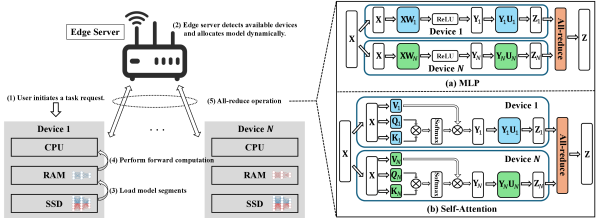
To deploy LLMs on resource-limited edge devices, distributed on-device inference with tensor parallelism has been proposed. This method involves partitioning large neural network tensors (e.g., weight matrices) of LLMs into smaller segments and distributing them across multiple edge devices for simultaneous processing. The complete workflow of the proposed distributed on-device LLM inference system is illustrated in Fig. 1. When a device initiates an inference request, the edge server dynamically identifies available local devices and partitions the model parameters. Then, each device loads its assigned model segment into memory and performs forward computation. After each layer of the LLM is computed, an all-reduce operation aggregates the intermediate layer outputs from all devices, ensuring synchronization and consistency across devices during inference. In the proposed distributed inference framework, the device shares its input (typically token embeddings rather than raw data) with other participating devices. For scenarios demanding strict confidentiality, encryption schemes (e.g., homomorphic encryption) or secure enclaves can be adopted to mitigate privacy leakage. Furthermore, we highlight two typical scenarios illustrating real-world, trusted environments particularly suitable for our distributed inference framework, as shown in the following.
-
•
Organizational or HPC Clusters: Large institutions (e.g., corporate data centers, national labs, or university HPC centers) often host massive LLMs that exceed the capacity of a single node. In these clusters, multiple servers within the same security domain can distribute model segments or layers among them, securely exchanging raw input data via internal networks. Since all compute nodes reside in the same trusted infrastructure (with well-defined access control, encryption, and compliance policies), they can fully leverage parallelization to reduce per-inference latency and alleviate memory bottlenecks, without risking data exposure to external environments.
-
•
Single-User or Local Edge Scenarios: Individual users or small teams may possess multiple personal devices or localized edge servers (e.g., the home server or on-premises GPU node). These devices operate within a single-user network or closed local environment, allowing them to share raw inputs without breaching privacy. By splitting the LLM’s parameters or layers across these trusted devices, users can achieve faster response times and reduced memory load per device. These benefits are especially valuable for real-time applications (e.g., smart home assistants or AR/VR), where offloading data to external clouds may be undesirable or impractical.
II-B Tensor Parallelism
LLMs are primarily built on the Transformer architecture, which typically consists of dozens of Transformer layers [45]. Each Transformer layer includes a self-attention mechanism and a multi-layer perceptron (MLP). To achieve efficient distributed inference, tensor parallelism partitions both the self-attention and MLP layers within each Transformer block into smaller tensor segments, as shown in Fig. 1. We note that both pipeline parallelism and tensor parallelism are two prevalent model partitioning strategies widely adopted in distributed inference frameworks. While pipeline parallelism partitions the model across layers, tensor parallelism partitions computations within each layer across multiple devices. Tensor parallelism is particularly attractive for on-device inference due to its inherent advantages in significantly reducing idle times (pipeline bubbles), achieving finer-grained memory allocation, and, when combined with AirComp-based aggregation, greatly minimizing communication overhead. These properties highlight the practical benefits and superior suitability of tensor parallelism for resource-constrained and latency-sensitive inference scenarios considered in this work.
II-B1 Tensor Parallelism for MLP Layer
For a typical 2-layer MLP within the Transformer block, the forward computation involves two main linear transformations, separated by a non-linear activation function (e.g., ReLU or GeLU). We formulate the computation of the MLP layer by taking the ReLU activation as an example. Mathematically, it is expressed as follows,
| (1) |
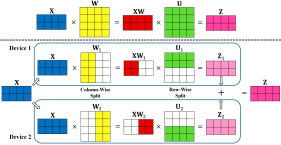
where is the input to the MLP layer, is the output, and and are the weight matrices, respectively. Our framework can be readily generalized to other activation functions, such as GeLU function: with representing the cumulative distribution function of the standard Gaussian distribution. The traditional centralized inference approach loads the entire weight matrices and into memory and performs full matrix multiplications on a single device, which is usually impractical for resource-limited edge devices. To overcome this challenge, tensor parallelism distributes the weight matrices and across devices. The weight matrices and have dimensions and , respectively. As shown in Fig. 2, the weight matrix is partitioned column-wise into multiple slices as
| (2) | ||||
where represents the portion of the weight matrix assigned to device and . Similarly, the weight matrix is partitioned row-wise as
| (3) |
where represents the portion of the weight matrix assigned to device . Then, each device can perform the forward computation on its respective model segment as follows,
| (4) |
where is the partial output produced by device . Once all devices obtain their local outputs , an all-reduce operation is performed to aggregate the partial outputs from all devices as follows,
| (5) |
The validity of this aggregation can be explained by considering how the model parameters are partitioned across the devices. Specifically, concatenating the column slices reproduces , and stacking the row slices recovers . Consequently, the original unpartitioned MLP output can be expressed as
| (6) | ||||
where (a) follows from the element-wise property of activation functions (e.g., ReLU, GeLU). Therefore, aggregating partial results reconstructs the original unpartitioned output (i.e., Eq. (5) holds). After aggregation, the final output of the MLP layer is broadcasted to all devices, ensuring synchronization and consistency across devices for the subsequent layer’s computation.
II-B2 Tensor Parallelism for Self-Attention Layer
For the self-attention layer, tensor parallelism similarly partitions its query (), key (), value (), and transformation () matrices across edge devices. In the traditional centralized computation of the self-attention layer, the output can be derived as follows,
| (7) |
where denotes the input, and denotes the dimension of the key vectors. In tensor parallelism, the memory-intensive weight matrices are splited and distributed across edge devices as follows,
| (8) | ||||
Then, each device performs local computation on its corresponding portion of the query, key, value, and transformation matrices as follows,
| (9) |
Once all devices obtain their local outputs , a similar all-reduce operation is required to gather and combine the partial outputs from devices as shown in (5).
II-C Over-the-Air All-Reduce
Employing tensor parallelism for distributed LLM inference requires frequent all-reduce operations, which cause significant communication overhead in practical wireless networks. To address this issue, we propose a communication-efficient AirComp all-reduce approach. The AirComp aggregates distributed data efficiently by leveraging the signal superposition property of wireless multiple-access channels, allowing simultaneous transmissions to compute nomographic functions (e.g., arithmetic mean) [46]. In the proposed distributed LLM inference system, the aggregation of intermediate layer outputs in the all-reduce step aligns with this operation, making the AirComp suitable to mitigate communication overhead. Note that edge devices performing AirComp must achieve symbol-level synchronization to ensure their transmitted signals arrive concurrently at the receiver, minimizing aggregation errors due to timing offsets. In our framework, synchronization among edge devices can be practically realized through the well-established timing advance (TA) mechanism. Specifically, the edge server estimates each device’s timing offset and instructs each device to adjust its signal transmission timing via dedicated TA commands. By aligning transmissions precisely, edge devices can ensure simultaneous arrival and accurate signal aggregation at the receiver.
We consider a wireless network consisting of an edge server with antennas and single-antenna edge devices. We further extend the proposed framework to a more general scenario invloving multi-antenna edge devices in Section IV. The uplink channels from edge devices to the server are block-fading, where channel statistics remain constant throughout the inference process, with channel states varying independently across different time intervals. Let denote the per-round transmitted entry of device ’s intermediate layer output , which has a complete dimensionality of . To reduce transmission power, the transmitted symbols are normalized to have zero mean and unit variance, i.e., , where the normalization factor is uniform for all devices and can be inverted at the server. Given synchronized symbol boundaries, all devices transmit their intermediate layer outputs simultaneously. To mitigate the distortion of received signals caused by channel noise, aggregation beamforming is adopted. Let denote the aggregation beamforming vector at the edge server. After the AirComp, the received signal at the server is given by,
| (10) |
where denotes the uplink channel from device to the server, is the transmit power of device , and denotes the additive white Gaussian noise vector with being the noise power. In the single-antenna setting, each device employs only a scalar transmit-power coefficient (instead of a beamforming vector) to scale its transmitted scalar entry . The distortion of with respect to the desired target summation is measured by the MSE, which is defined as
| (11) |
The MSE serves as a metric to evaluate the performance of the AirComp all-reduce operations. As shown in the simulations later, the inference accuracy of the distributed on-device LLM inference system is greatly influenced by the transmission error during the AirComp phase. By substituting (10) into (11), the MSE can be explicitly represented as a function of aggregation beamforming vector and transmitter scalars as follows,
| (12) |
Edge devices involved in inference tasks typically have limited energy supply. Thus, we assume that for each device , the energy consumption for both the forward computation of each LLM layer and the transmission of the intermediate output cannot exceed the maximum power budget . To model the computation energy consumption, we first introduce a model assignment vector with its entry representing the proportion of model allocated to device . Consequently, the computation energy consumption for device is given by , where denotes the device-specific energy coefficient that reflects the energy cost associated with accessing and processing each weight during computation, and is the number of parameters (weights) for each layer. The communication energy consumption of device can be derived as . Accordingly, the power constraint is given by
| (13) |
II-D Problem Formulation
In the proposed distributed LLM inference system, the overall performance is determined by the model assignment policy and the transceiver design , . Optimal model assignment ensures that each device processes a suitable portion of the model based on its computational capability (e.g., memory size and compute power). Meanwhile, efficient transceiver optimization can reduce signal misalignment error and suppress channel noise, thereby improving inference accuracy. Thus, to improve inference performance, we formulate a joint model assignment and transceiver optimization problem that aims to minimize the average MSE, subject to the per-device power constraints. Importantly, the transceiver design can adapt dynamically to instantaneous CSI. In contrast, adapting the model assignment policy to instantaneous CSI in a real-time manner is impractical due to the significant latency caused by loading different model segments. Thus, model assignment should be finished before inference based on the long-term channel statistics.
The resulting problem is therefore formulated as a mixed-timescale joint optimization of the short-term transceiver variables , and the long-term model assignment policy as follows,
| (14) | ||||
| s.t. | ||||
where the expectation is taken over all random channel realizations . However, the problem is challenging to be solved due to the following three reasons.
-
•
Non-convexity: The objective function is inherently non-convex due to the coupling between the receiver aggregation beamformer and the transmitter scalars .
-
•
Expectation over Random Channels: The objective involves an expectation over random CSI, which requires prior knowledge of channel statistics.
-
•
Interdependence of Timescales: The per-device power constraints link the short-term transceiver variables with the long-term model assignment policy, leading to a complex interplay between the two timescales.
To address these challenges, we develop a two-stage algorithm that separately solves the short-term transceiver optimization and the long-term model assignment optimization in the following section.
III Algorithm Development
In this section, we develop an efficient two-stage algorithm to solve the joint model assignment and transceiver optimization problem . Then, we show that the proposed algorithm can converge to a stationary point of the original problem .
III-A Problem Decomposition
We start by decomposing problem into a family of short-term transceiver optimization problems and a long-term model assignment optimization problem as follows.
III-A1 Short-term transceiver optimization for given model assignment policy and channel condition
| (15) | ||||
| s.t. |
III-A2 Long-term model assignment optimization based on the optimal solution to problem
| (16) | ||||
| s.t. | ||||
The short-term transceiver optimization problem remains non-convex, and we address it using the SDR technique. The long-term model assignment optimization problem is similarly challenging, as the optimal transceiver variables cannot be derived in closed form. Additionally, the distribution of CSI is difficult to obtain in practical wireless systems. To address these challenges, we propose a stochastic SCA algorithm that operates without requiring prior knowledge of channel statistics. In the following subsections, we provide a detailed implementation of the proposed algorithms.
III-B Short-Term Transceiver Optimization for
The short-term problem is challenging to be solved due to the inherent non-convexity caused by the coupling between receiver aggregation beamformer and the transmitter scalers . Thus, we first simplify problem by demonstrating that the channel inversion precoding is optimal conditioned on the aggregation beamformer.
Lemma 1.
For a given aggregation beamformer , the transmission MSE is minimized by using the zero-forcing precoders .
Proof.
Let represent the normalized aggregation beamformer that satisfies , and consequently where is optimized to satisfy the power constraints of edge devices. By applying Lemma 1, problem can be reformulated as follows,
| (17) | ||||
| s.t. | ||||
Then, by employing the equation , an equivalent formulation of problem (17) is obtained as follows,
| (18) | ||||
| s.t. | ||||
The problem (18) remains intractable due to the non-convex norm constraint on . To address this issue, we apply the SDR approach that relaxes the non-convex norm constraint by employing its convex hull.
Lemma 2.
(Convex Hull Relaxation [48]) Suppose the set and set , where is of the size by while is of the size by . The condition of the set indicates that both and are positive semi-definite. Then, is the convex hull of , and is the set of extreme points of .
By applying Lemma 2, we can replace the non-convex norm constraint by its convex hull and reformulate a relaxed version of problem (18) as follows,
| (19) | ||||
| s.t. | ||||
where . The problem (19) can be proved to be convex, and the globally optimal solution can be obtained by using a convex solver (e.g., the CVX toolbox in MATLAB [49]).
We note that the optimal solution has a high probability to satisfy the rank-one constraint [47]. If a rank-one solution is obtained, the optimal solution of the original problem (18) can be immediately achieved by extracting the dominant eigenvector of as . Otherwise, if the rank of is larger than 1, we apply the Gaussian randomization algorithm [50] to map the solution to a feasible, near-optimal solution for the original non-convex problem.
III-C Long-Term Model Assignment Optimization for
In this subsection, we propose a stochastic SCA algorithm to solve the long-term model assignment problem . The proposed algorithm requires no prior knowledge of channel statistics. For clearer algorithmic description, we first reformulate the long-term problem into an equivalent form as follows,
| (20) | ||||
| s.t. | ||||
where , and . The proposed stochastic SCA algorithm iteratively performs the following two steps: First, quadratic surrogate functions , are constructed to approximate the non-convex components of the original objective and constraint functions , , respectively. Then, the resulting convex quadratic approximation problem is solved, and the long-term model assignment policy is updated based on the solution. The details of these two steps are illustrated as follows.
III-C1 Step 1
In each iteration , the edge server first generates a channel sample , and then calculates the short-term transceiver variables and by solving the short-term problem . Then, the recursive convex approximation of the original objective function can be derived as[51]
| (21) |
where is a constant that ensures convexity, denotes the sample-wise approximation of the average MSE and is computed by using the specific channel realization . Furthermore, is an approximation of the gradient , which is updated recursively as
| (22) |
and [51]. The algorithm parameter is decreasing in , satisfying , , , and . Similarly, the recursive convex approximation of the power constraint function is given by
| (23) |
where is a constant, and is updated recursively as follows[51],
| (24) |
It is noted that the surrogate functions and are quadratic approximations of the original nonconvex objective and constraint around the current iterate . Specifically, at iteration , each surrogate function is constructed using first-order Taylor expansions of the corresponding function (for ), along with an additional quadratic regularization term controlled by convexity constants and . The convexity constants and serve to ensure strong convexity and numerical stability of the surrogate functions. Specifically, larger values of and enhance numerical stability but may slow convergence, whereas smaller values permit larger update steps but require careful tuning to prevent instability. In practice, setting these constants within the range (e.g., around 0.05) achieves a favorable balance between stability and convergence speed.
III-C2 Step 2
After obtaining the convex approximations of the objective and constraint functions, we formulate a convex approximation of the original problem (20) to solve the optimal as follows,
| (25) | ||||
| s.t. | ||||
If problem (25) turns out to be infeasible, the optimal solution is obtained by solving the following feasibility problem,
| (26) | ||||
| s.t. | ||||
After solving for , the model assignment policy is updated as
| (27) |
where satisfies , , and [51]. To facilitate practical implementation and reproducibility, we provide explicit heuristics for choosing the hyperparameters and . We suggest setting these hyperparameters as and , where the parameter typically ranges from 0.5 to 1 to satisfy the convergence conditions outlined in Lemma 3. In practice, setting , , and has been found through simulations to achieve an effective balance between convergence speed and numerical stability.
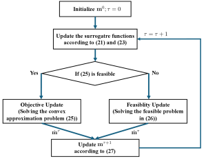
The above two steps iterate until convergence, i.e., , where is the convergence tolerance. The overall algorithm is outlined in Algorithm 1, and the block diagram of the proposed algorithm is illustrated in Fig. 3.
Remark 1.
The computational complexity of solving the short-term transceiver optimization problem is at most , and is usually much lower in practice [52, Theorem 3.12]. Moreover, the most computation-expensive steps for the long-term optimization problem are solving the constructed convex quadratic approximation problems (25) and (26). Specifically, the computational complexity of solving problems (25) and (26) is at most in the order of . Then, the total computational complexity of Algorithm 1 is given by , where is the maximum iteration number of Algorithm 1. Both optimization and model assignment are performed only once at the beginning of the inference (or after substantial changes in channel or device conditions). Hence, while solving the optimization and loading model segments introduce a non-negligible one-time cost, the subsequent benefits from parallelized forward computation significantly outweigh this initial overhead, resulting in increased inference speed in practical settings.
Remark 2.
In the proposed framework, the edge server, which possesses limited but non-negligible computational and memory resources, collects the channel state information and device capability information. Leveraging these data, the server solves the mixed-timescale optimization problem and assigns each participating edge device its respective portion of the model parameters.
III-D Convergence Analysis
In this subsection, we analyze the asymptotic convergence performance of Algorithm 1 to a stationary point of the original problem .
We first show the convergence of the surrogate functions in the following lemma.
Lemma 3.
Consider a sequence converging to a limiting point , and define
| (28) | ||||
which satisfies and . Then, if the algorithm parameter satisfies , we have
| (29) | ||||
almost surely[51].
Proof.
The proof is presented in Appendix A. ∎
To elaborate the convergence result, we need to introduce the Slater’s condition for the converged surrogate function in the following.
Definition 1.
(Slater’s Condition) Given the sequence converging to a limiting point and let be the converged surrogate function as defined in (28). The Slater’s condition holds at if there exists a constant such that
| (30) | ||||
The Slater’s condition is widely used in constrainted optimization algorithms (e.g., the majorization-minimization algorithm [53] and virtual queue-based online convex optimization algorithm [54]). With Lemma 3 and the Slater’s condition, we are ready to show the main convergence result of Algorithm 1 in the following theorem.
Theorem 1.
Let denote the sequence of model assignment policies generated by Algorithm 1. If the Slater’s condition is satisfied at the limiting point of the sequence , then is a stationary point of problem almost surely.
Proof.
The proof is presented in Appendix B. ∎
In Section V-B, we further verify the convergence of Algorithm 1 through simulations.
IV Extension to Multi-Antenna Devices
In the previous sections, we analyzed the scenario of single-antenna edge devices to establish foundational insights for optimizing communication efficiency in distributed LLM inference. In this section, we extend the proposed framework and algorithms to the multi-antenna setting. By leveraging spatial multiplexing, the multi-antenna configuration further enhances communication efficiency and reduces inference latency, providing a more general and scalable solution.
IV-A Problem Formulation
Building upon the single-antenna setting, we now consider a more generalized scenario where edge devices in the distributed LLM inference system are equipped with multiple antennas. Thus, the spatial diversity and spatial multiplexing are utilized to further improve communication efficiency. Specifically, we consider the server and each edge device are equipped with and antennas, respectively. Similar to the single-antenna case, all devices simultaneously upload their intermediate layer outputs through wireless multiple-access channels. Let denote the per-round transmitted entries of device ’s intermediate output . Let and denote the aggregation beamforming matrix at the edge server and the data precoding matrix at device , respectively. Then, the received signal at the server after the AirComp can be derived as follows,
| (31) |
where denotes the uplink MIMO channel from device to the edge server. In the multi-antenna setting, each device employs the precoding (beamforming) matrix to map its transmitted vector onto multiple antennas for simultaneous transmission. The distortion of with respect to the desired target vector is measured by the MSE, defined as
| (32) |
By substituting (31) into (32), the MSE can be explicitly represented as a function of transceiver beamforming matrices as follows,
| (33) | ||||
To effectively utilize the heterogeneous computational capabilities of edge devices and mitigate communication distortions, we similarly investigate a joint model assignment and transceiver optimization problem. Specifically, the joint optimization problem in the multi-antenna scenario can be formulated as follows,
| (34) | ||||
| s.t. | ||||
where the expectation is taken over all random channel realizations .
IV-B Algorithm Development
In this subsection, we extend Algorithm 1 to a more general case involving multi-antenna edge devices. Similarly, we first decompose problem into a family of short-term subproblems and a long-term subproblem as follows.
IV-B1 Short-term transceiver optimization for given model assignment policy and channel condition
| (35) | ||||
| s.t. |
IV-B2 Long-term model assignment optimization based on the optimal solution to problem
| (36) | ||||
| s.t. | ||||
To solve the short-term problem , we first simplify it by demonstrating that the zero-forcing (channel inversion) precoder is optimal conditioned on the aggregation beamformer.
Lemma 4.
For a given aggregation beamformer , the transmission MSE is minimized by using the zero-forcing precoders as follows,
| (37) |
Let represent the normalized aggregation beamformer that satisfies , and consequently with denoting the norm of . By employing (37), the problem can be reformulated as follows,
| (38) | ||||
| s.t. | ||||
The problem (38) remains challenging to be solved due to its non-convex constraints involving the term . To address this issue, we develop a tractable approximation of the problem by employing the following inequality,
| (39) |
where the equality holds when the channel is well-conditioned, i.e., the singular values of are identical. By utilizing (39), we reformulate an approximated version of problem (38) as follows,
| (40) | ||||
| s.t. | ||||
Then, by introducing a new variable , an equivalent formulation of problem (40) is obtained as follows,
| (41) | ||||
| s.t. | ||||
We observe that the only non-convex constraint in problem (41) is . Therefore, we remove this constraint to obtain a relaxed version of problem (41) as follows,
| (42) | ||||
| s.t. | ||||
The problem (42) can be proved to be a convex problem. After solving problem (42) using a convex solver (e.g., the CVX toolbox in MATLAB [49]) and obtaining the globally optimal solution , we apply the Gaussian randomization algorithm [50] to map the solution to a feasible, near-optimal solution for the original non-convex problem.
Next, we solve the long-term model assignment problem . The proposed stochastic SCA algorithm, initially introduced for the single-antenna case in Section III-B, can be directly extended to the multi-antenna scenario without requiring further modifications. For clearer algorithmic description, we first reformulate the long-term problem into an equivalent form as follows,
| (43) | ||||
| s.t. | ||||
where
, and . The main structure of the proposed stochastic SCA algorithm remains intact, and it iteratively performs the following two steps: First, quadratic surrogate functions , are constructed to approximate the non-convex components of the original objective and constraint functions , , respectively. Then, the resulting convex quadratic approximation problem is solved, and the long-term model assignment policy is updated based on the solution. Here, we omit the details of these two steps for brevity. In Section V-B, we also demonstrate the convergence of the proposed algorithm for the multi-antenna scenario through simulations.
V Simulation Results
V-A Simulation Setups
V-A1 LLM Inference Model Setting
All simulations are performed on a desktop server equipped with Nvidia GeForce RTX 4070Ti GPU and Intel Core i9 CPU, using PyTorch 2.0 with CUDA 11.7. We set up virtual machines (VMs) with each VM simulating a distinct edge device. Each VM is allocated 4 CPU cores, 16 GB RAM, and 128 GB storage space, ensuring efficient utilization of computational resources and optimized parallel processing. For evaluation, we utilize the LLaMA2 [55] and LLaMA3 [11] models due to their state-of-the-art performance among open-source models. Additionally, we employ the WikiText-2 dataset [56], which is widely used in the field of LLM inference for benchmarking and evaluation purposes. We have released our implementation on GitHub: https://github.com/zklasd24/distributed_llama_AirComp, which builds upon the open-source project Distributed Llama [57].
The primary performance metric for inference accuracy is perplexity [58], which is a widely recognized measure of a LLM’s capability to predict the next word in a sequence. It is defined mathematically as follows,
| (44) |
where denotes the model’s predicted probability for the next word , and is the text length. Lower perplexity values indicate better inference performance, reflecting the model’s accuracy in generating subsequent tokens.
V-A2 Communication Model Setting
The number of antennas at the edge server is , and each edge device has single antenna or antennas for different cases. The bandwidth between the edge server and edge devices is MHz. The uplink channels are assumed to be independent and identically distributed (i.i.d.) Rician fading [59], modeled as i.i.d. complex Gaussian random variables with non-zero mean and variance . Moreover, the maximum power budget is set as and the noise variance at the edge server is assumed to be 1.
V-B Algorithm Convergence
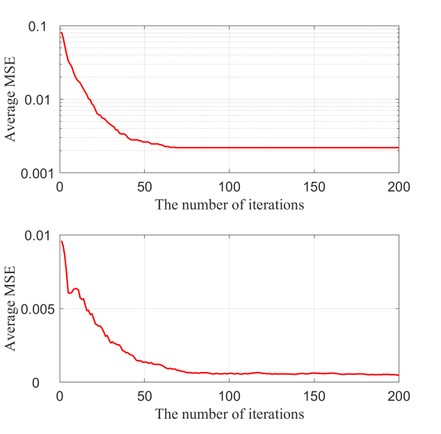
In this subsection, we analyze the convergence behavior of the propose d algorithm for both single-antenna and multi-antenna scenarios. The parameter parameters are set as , , and . As illustrated in Fig. 4, the proposed algorithm demonstrates rapid convergence, reaching a stationary point within approximately 100 iterations. The swift convergence speed ensures that the distributed LLM inference system can quickly adapt to varying network conditions, enabling real-time inference especially in latency-sensitive applications. Moreover, the consistent performance across both single-antenna and multi-antenna settings suggests the robustness of the proposed algorithm to various network scenarios.
V-C Performance Evaluation
In this subsection, we compare the performance of the proposed AirComp all-reduce approach with the following two benchmark schemes.
-
•
Digital All-Reduce: All devices upload intermediate layer outputs using a traditional broadband digital multiple-access scheme, with each transmitted symbol quantized to bits. To prevent multi-user interference, orthogonal frequency division multiple-access (OFDMA) is employed, assigning each sub-channel to one device [60].
-
•
Uncoded FDMA: This scheme similarly employs the OFDMA technique, with each device occupying a dedicated sub-channel to upload intermediate layer outputs in an uncoded analog manner.
| Transmission Scheme | Transmission Time |
| Digital All-Reduce | |
| Uncoded FDMA | |
| AirComp All-Reduce |
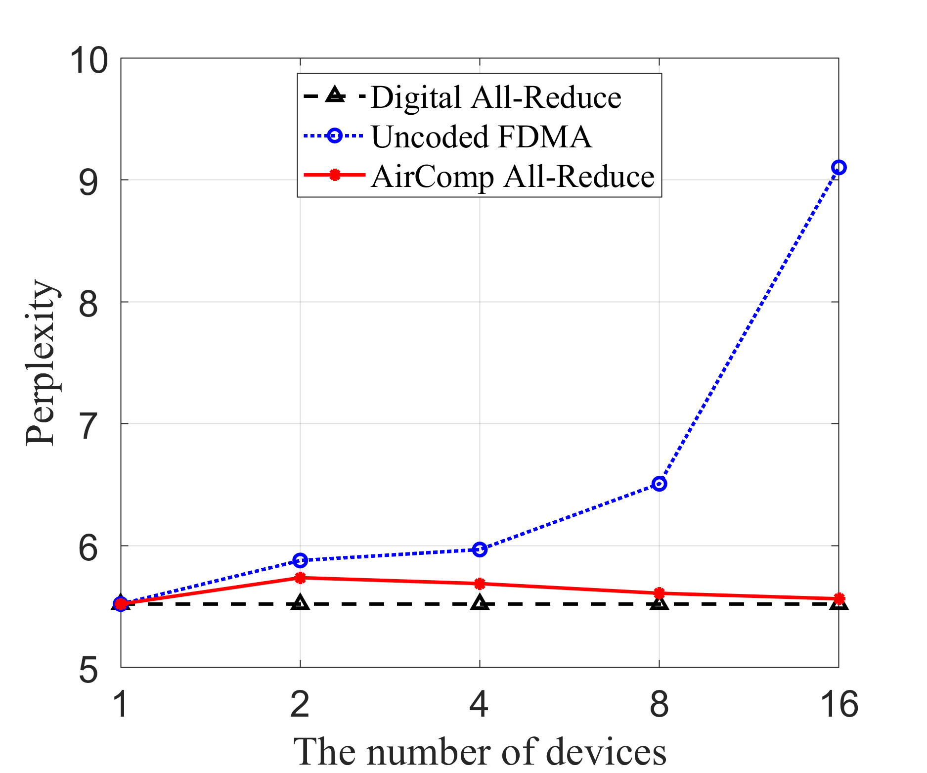
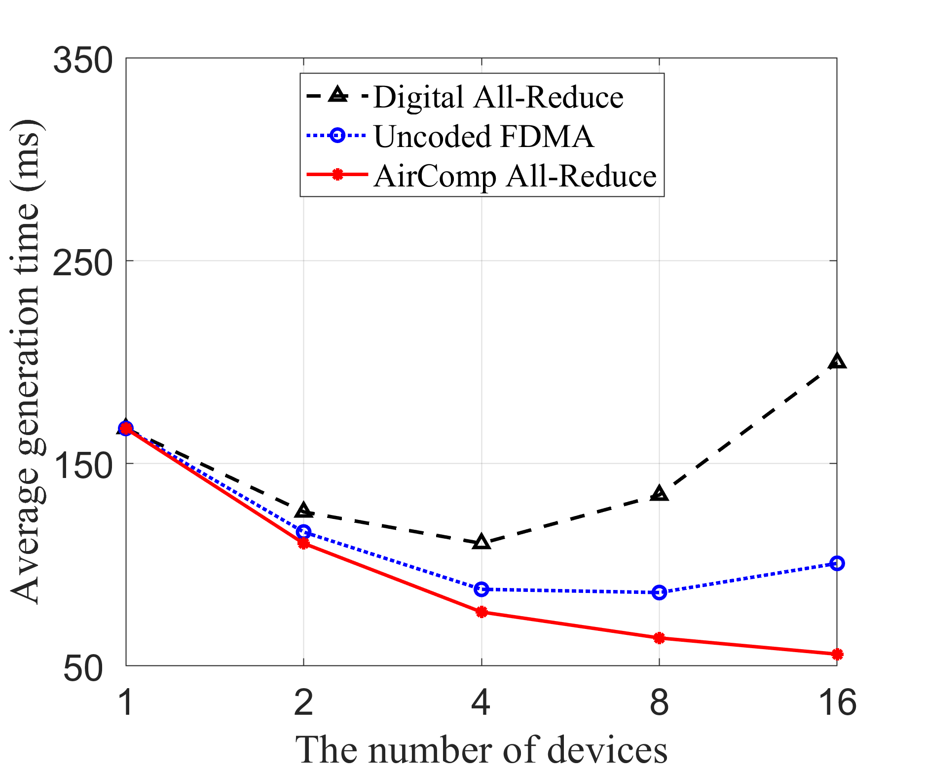
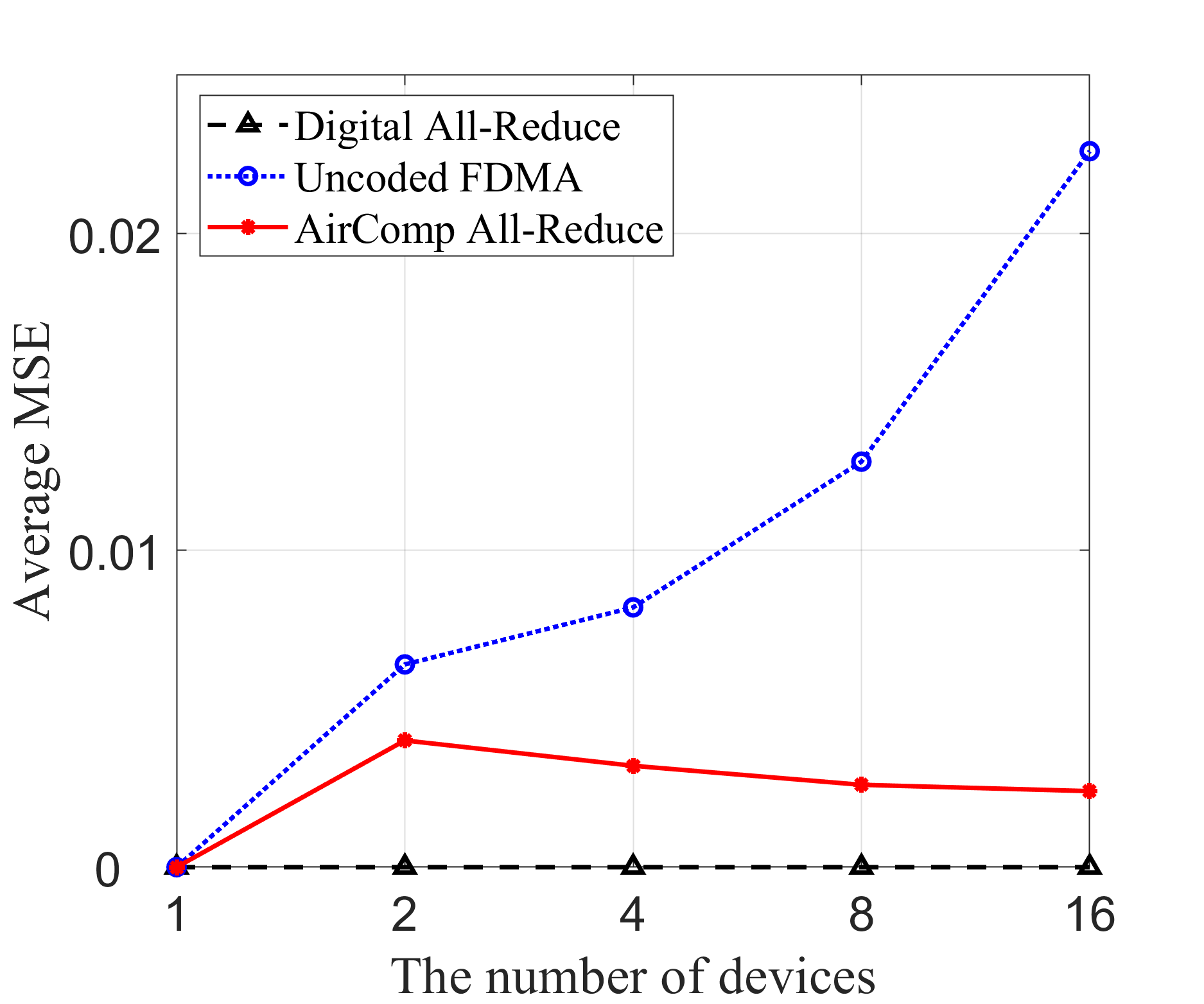
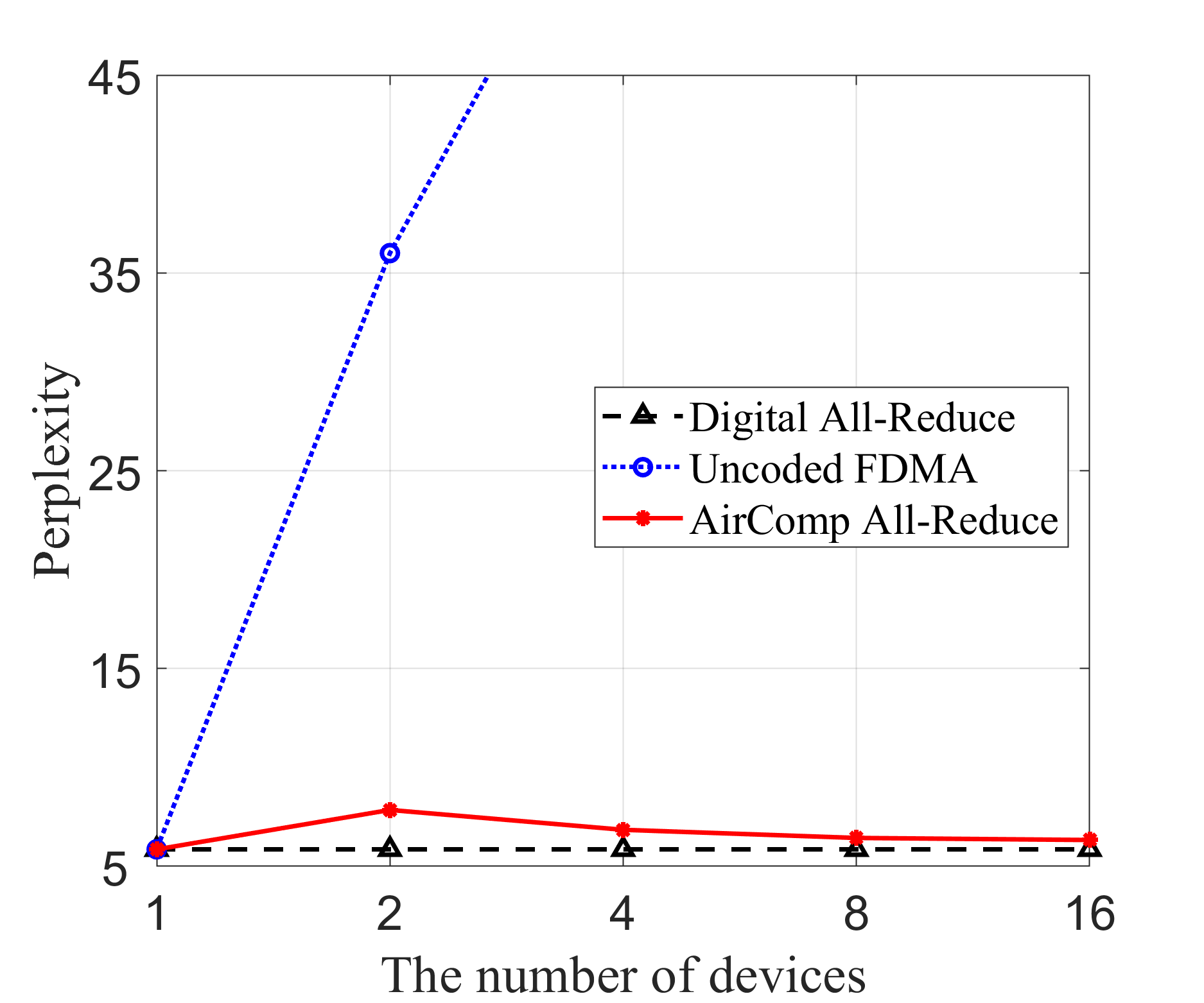
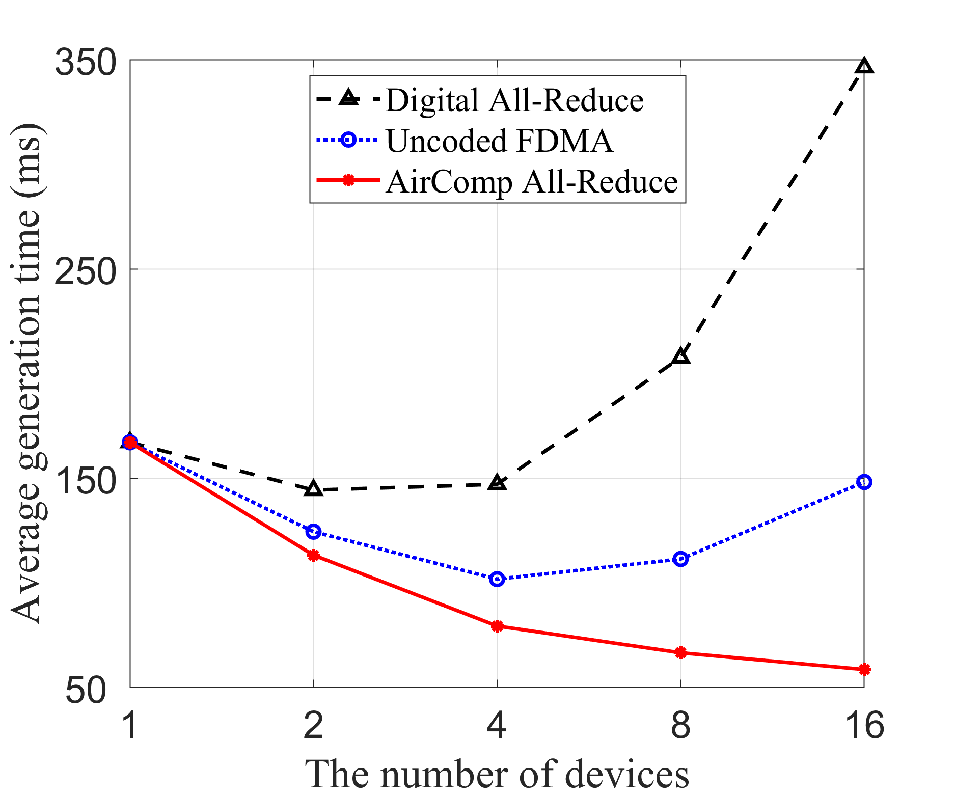
In Fig. 5, we compare the inference performance of different transmission schemes using the LLaMA3 model with 8 billion parameters, across three key performance metrics: transmission MSE, perplexity, and average generation time. In Fig. 5(a), the proposed AirComp all-reduce approach consistently achieves low MSE across all device counts, significantly outperforming the uncoded FDMA scheme, which exhibits a near-linear increase in MSE as the number of devices grows. The digital all-reduce method achieves near-zero MSE across all configurations. However, it has significantly higher communication latency. In Fig. 5(b), perplexity follows the same trend as the transmission MSE. The AirComp all-reduce method maintains stable, low perplexity across all device configurations, while the perplexity of uncoded FDMA rises sharply with more devices. Digital all-reduce performs similarly to AirComp all-reduce, maintaining low perplexity. Turning to the average generation time in Fig. 5(c), we observe a notable distinction among the three methods. Here, the total inference time is defined as the sum of local computation time and the time taken to transmit the local outputs. The local computation time is obtained through experimental measurements, while the communication time is estimated based on different transmission methods as outlined in Table II, where denotes the average receive signal-to-noise ratio (SNR). We observe that AirComp all-reduce consistently demonstrates the lowest latency, particularly as the number of edge devices grows. The digital all-reduce scheme shows a significant increase in generation time with more devices due to increased communication overhead, while the uncoded FDMA method provides moderate improvements but still lags behind AirComp all-reduce. The proposed AirComp all-reduce approach exhibits superior scalability compared to traditional communication strategies. Specifically, by exploiting analog signal superposition inherent in wireless channels, AirComp enables simultaneous aggregation of signals from multiple devices within a single communication slot. Consequently, unlike traditional communication schemes, whose overhead increases linearly with the number of participating devices, the AirComp all-reduce approach maintains low communication latency even as device count grows.
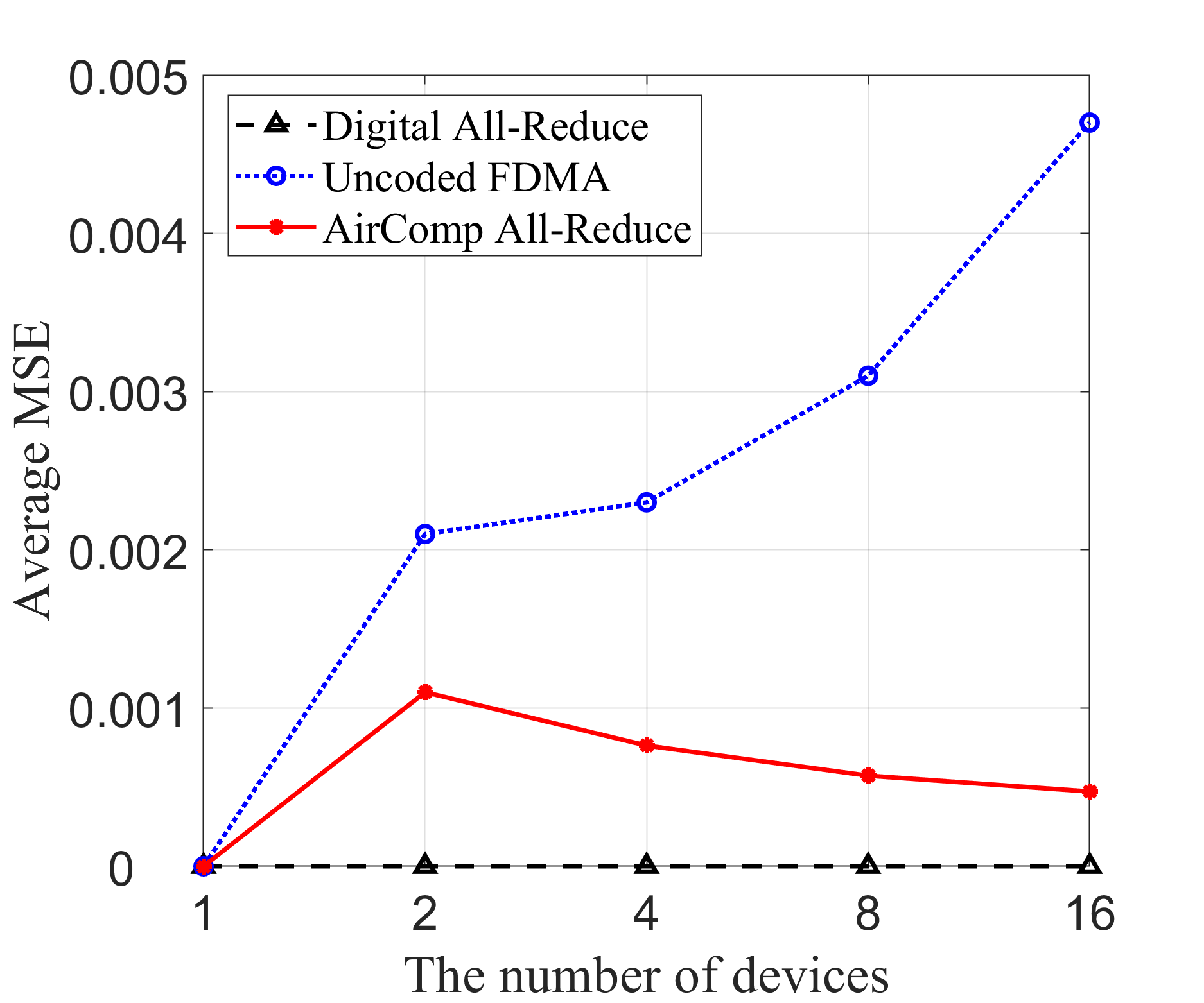
Fig. 6 expands on the simulation results by evaluating the performance of the proposed method in a more general setting of multi-antenna devices. In this scenario, the digital all-reduce scheme maintains the lowest MSE and perplexity. However, its average generation time grows considerably with an increasing number of devices, indicating scalability limitations in practice. The proposed AirComp all-reduce scheme, while exhibiting a slight increase in MSE compared to digital all-reduce, remains competitive in terms of perplexity and demonstrates the shortest generation time across all configurations. This makes it an promising choice for applications where low latency is critical, and slight trade-offs in accuracy are acceptable. On the other hand, the uncoded FDMA scheme’s performance degrades significantly with more devices, reflected by steep increases in both MSE and perplexity.
| Average generation time per token (ms) | ||||||||||||||||
| Model | LLaMA2-7B | LLaMA2-13B | LLaMA2-70B | LLaMA3-70B | ||||||||||||
| Device Number | 1 | 2 | 4 | 8 | 1 | 2 | 4 | 8 | 1 | 2 | 4 | 8 | 1 | 2 | 4 | 8 |
| Digital All-Reduce | 114.2 | 85.2 | 79.5 | 108.3 | 217.3 | 174.0 | 176.6 | 261.4 | 807.3 | 729.7 | 981.6 | N/A | 893.2 | 783.8 | 1033.6 | |
| AirComp All-Reduce | 114.2 | 69.7 | 45.7 | 37.8 | 217.3 | 128.5 | 81.3 | 66.4 | N/A | 660.9 | 423.0 | 354.2 | N/A | 746.8 | 477.1 | 406.0 |
| *: Not available due to insufficient memory. | ||||||||||||||||
To further validate the effectiveness of the proposed algorithm, we conduct additional experiments using larger models, including LLaMA2 with 7, 13, and 70 billion parameters, and LLaMA3 with 70 billion parameters. In Table III, it is observed that AirComp all-reduce method consistently demonstrates superior performance in terms of reduced generation time, particularly as the number of devices increases. Across various device and model configurations, AirComp all-reduce achieves up to 4x faster generation speed, demonstrating its significant advantages for distributed LLM inference, especially with large-scale models.
Overall, the AirComp all-reduce approach emerges as a balanced and scalable solution, effectively managing the trade-offs between latency, accuracy, and scalability in both single-antenna and multi-antenna environments. This highlights its potential for deployment in practical, large-scale wireless scenarios.
V-D Comparison with Centralized Inference Approach
In this subsection, we compare the proposed AirComp-based distributed inference framework with the traditional centralized inference approach. Table IV compares the per-token generation latency for centralized versus distributed LLM inference across different large models. As shown in the table, although the centralized inference does not incur a communication overhead, it suffers from significantly higher per-token computation time. In contrast, the proposed distributed inference approach partitions the model across multiple devices, substantially reducing each device’s computational load. Despite introducing modest communication overhead, the proposed distributed scheme achieves significantly lower total inference latency per token. Hence, for large-scale LLMs with billions of parameters, distributing both the model storage and compute cost across multiple devices proves far more feasible and efficient than hosting the entire model on a single node. Moreover, both per-token local computation time and communication overhead increase substantially as the number of transformer layers grows. However, it is noteworthy that the distributed inference approach consistently maintains a significant latency advantage over centralized inference across all models with different number of layers.
| Model | Number of Transformer Layers | Method | Per-Token Local Computation Time (ms) | Per-Token Communication Time (ms) | Per-Token Total Generation Time (ms) |
| LLaMA2-7B | 32 | Centralized | 114.2 | 0 | 114.2 |
| Distributed | 26.0 | 11.8 | 37.8 | ||
| LLaMA2-13B | 40 | Centralized | 217.3 | 0 | 217.3 |
| Distributed | 38.5 | 27.9 | 66.4 | ||
| LLaMA2-70B | 80 | Centralized | 1152.6 | 0 | 1152.6 |
| Distributed | 264.6 | 89.6 | 354.2 |
VI Conclusion
In this paper, we proposed a novel distributed on-device LLM inference framework employing tensor parallelism. To mitigate the communication overhead from frequent all-reduce steps in tensor parallelism, we proposed a communication-effcient AirComp all-reduce approach. Moreover, to minimize the average transmission MSE, we formulated a joint model assignment and transceiver design problem, which can be derived as a mixed-timescale stochastic non-convex optimization. We further developed an efficient two-stage algorithm that decomposed the original problem in short-term transceiver optimization and long-term model assignment optimization problems, which were solved by leveraging the SDR and stochastic SCA, respectively. We proved that the proposed algorithm can converge almost surely to a stationary point of the original problem. Simulation results demonstrated that the proposed approach significantly reduced inference latency while improving inference accuracy, making distributed on-device LLM inference feasible for resource-constrained edge devices.
There are several promising directions for further advancing distributed on-device LLM inference systems. One important research direction is experimentally validating the proposed AirComp-based distributed inference framework using real-world wireless hardware setups, further assessing practical performance and robustness. In addition, exploring cluster-based hierarchical AirComp designs and distributed transceiver optimization methods can effectively address potential scalability bottlenecks arising from synchronization overhead, channel estimation complexity, and computational demands in large-scale device networks.
Appendix
VI-A Proof of Lemma 3
According to the assumption that channel statistics remain constant throughout the inference process, we have that the sample-wise approximation of the average MSE, , satisfying
| (45) |
| (46) |
which follow from the law of large numbers and the central limit theorem, respectively. Then, combining (45) and (46) into (21), we have
| (47) |
for . Equation (47) indicates the convergence of , and we then need to prove the convergence of as follows,
| (48) |
It is easy to verify that the MSE funtion and its derivation are Lipschitz continuous, according to the fact that the channel sample is always bounded in practice. Then, we can obtain that
| (49) | ||||
where (a) holds since is Lipschitz continuous. From , we can obtain that
| (50) |
which indicates the convergence of . Then, according to [61, Lemma 1], equation (48) holds.
Next, according to the fact that is Lipschitz continuous, it directly follows that there exists a constant such that
| (51) |
VI-B Proof of Theorem 1
Let denote the sequence of model assignment policies generated by Algorithm 1. According to [51, Lemma 4], we have
| (52) |
| (53) |
where is obtained by solving problem (25) or (26). Then, we introduce an auxiliary variable , which is the optimal solution of the following problem,
| (54) | ||||
| s.t. | ||||
where . Letting in (54) and combining (47) and (53) into (54), we have
| (55) | ||||
| s.t. | ||||
Then, if satisfies the Slater’s condition, we have that the KKT condition of problem (55) holds, i.e., there exists such that
| (56) |
Finally, it follows from Lemma 1 and (56) that satisfies the KKT condition of the original problem as follows,
| (57) |
This completes the proof.
References
- [1] K. Zhang, H. He, S. Song, J. Zhang, and K. B. Letaief, “Distributed on-device LLM inference with over-the-air computation,” in Proc. IEEE Int. Conf. Commun. (ICC), Montreal, Canada, Jun. 2025, to appear, https://arxiv.org/abs/2502.12559.
- [2] B. Min, H. Ross, E. Sulem, A. P. B. Veyseh, T. H. Nguyen, O. Sainz, E. Agirre, I. Heintz, and D. Roth, “Recent advances in natural language processing via large pre-trained language models: A survey,” ACM Comput. Surv., vol. 56, no. 2, pp. 1–40, 2023.
- [3] Y. Chang, X. Wang, J. Wang, Y. Wu, L. Yang, K. Zhu, H. Chen, X. Yi, C. Wang, Y. Wang, et al., “A survey on evaluation of large language models,” ACM Trans. Intell. Syst. Technol., vol. 15, no. 3, pp. 1–45, 2024.
- [4] Y. Gu, R. Tinn, H. Cheng, M. Lucas, N. Usuyama, X. Liu, T. Naumann, J. Gao, and H. Poon, “Domain-specific language model pretraining for biomedical natural language processing,” ACM Trans. Comput. Healthc., vol. 3, no. 1, pp. 1–23, 2021.
- [5] H. Fan, X. Liu, J. Y. H. Fuh, W. F. Lu, and B. Li, “Embodied intelligence in manufacturing: leveraging large language models for autonomous industrial robotics,” J. Intell. Manuf., pp. 1–17, 2024.
- [6] Y. Yang, T. Zhou, K. Li, D. Tao, L. Li, L. Shen, X. He, J. Jiang, and Y. Shi, “Embodied multi-modal agent trained by an LLM from a parallel textworld,” in IEEE Conf. Comput. Vis. Pattern Recognit., pp. 26275–26285, 2024.
- [7] D. Driess, F. Xia, M. S. Sajjadi, C. Lynch, A. Chowdhery, B. Ichter, A. Wahid, J. Tompson, Q. Vuong, T. Yu, et al., “Palm-e: An embodied multimodal language model,” arXiv preprint arXiv:2303.03378, 2023.
- [8] L. Bariah, Q. Zhao, H. Zou, Y. Tian, F. Bader, and M. Debbah, “Large generative AI models for telecom: The next big thing?,” IEEE Commun. Mag., 2024.
- [9] J. Shao, J. Tong, Q. Wu, W. Guo, Z. Li, Z. Lin, and J. Zhang, “WirelessLLM: Empowering large language models towards wireless intelligence,” J. Commun. Inf. Netw., vol. 9, pp. 99–112, 2024.
- [10] J. Tong, J. Shao, Q. Wu, W. Guo, Z. Li, Z. Lin, and J. Zhang, “WirelessAgent: Large language model agents for intelligent wireless networks,” arXiv preprint arXiv:2409.07964, 2024.
- [11] A. Dubey, A. Jauhri, A. Pandey, A. Kadian, A. Al-Dahle, A. Letman, A. Mathur, A. Schelten, A. Yang, A. Fan, et al., “The llama 3 herd of models,” arXiv preprint arXiv:2407.21783, 2024.
- [12] B. Wu, Y. Zhong, Z. Zhang, G. Huang, X. Liu, and X. Jin, “Fast distributed inference serving for large language models,” arXiv preprint arXiv:2305.05920, 2023.
- [13] A. Borzunov, M. Ryabinin, A. Chumachenko, D. Baranchuk, T. Dettmers, Y. Belkada, P. Samygin, and C. A. Raffel, “Distributed inference and fine-tuning of large language models over the internet,” Adv. Neural Inf. Process. Syst., vol. 36, 2024.
- [14] C. Hu, H. Huang, L. Xu, X. Chen, J. Xu, S. Chen, H. Feng, C. Wang, S. Wang, Y. Bao, et al., “Inference without interference: Disaggregate llm inference for mixed downstream workloads,” arXiv preprint arXiv:2401.11181, 2024.
- [15] K. B. Letaief, W. Chen, Y. Shi, J. Zhang, and Y.-J. A. Zhang, “The roadmap to 6G: AI empowered wireless networks,” IEEE Commun. Mag., vol. 57, no. 8, pp. 84–90, 2019.
- [16] K. B. Letaief, Y. Shi, J. Lu, and J. Lu, “Edge artificial intelligence for 6G: Vision, enabling technologies, and applications,” IEEE J. Sel. Areas Commun., vol. 40, no. 1, pp. 5–36, 2021.
- [17] M. Zhang, J. Cao, X. Shen, and Z. Cui, “Edgeshard: Efficient LLM inference via collaborative edge computing,” arXiv preprint arXiv:2405.14371, 2024.
- [18] X. Yuan, N. Li, T. Zhang, M. Li, Y. Chen, J. F. M. Ortega, and S. Guo, “High efficiency inference accelerating algorithm for noma-based edge intelligence,” IEEE Trans. Wireless Commun., 2024.
- [19] Y. He, J. Fang, F. R. Yu, and V. C. Leung, “Large language models inference offloading and resource allocation in cloud-edge computing: An active inference approach,” IEEE Trans. Mobile Comput., 2024.
- [20] Y. Chen, R. Li, X. Yu, Z. Zhao, and H. Zhang, “Adaptive layer splitting for wireless LLM inference in edge computing: A model-based reinforcement learning approach,” arXiv preprint arXiv:2406.02616, 2024.
- [21] J. Shao, Y. Mao, and J. Zhang, “Learning task-oriented communication for edge inference: An information bottleneck approach,” IEEE J. Sel. Areas Commun., vol. 40, no. 1, pp. 197–211, 2021.
- [22] H. Li, W. Yu, H. He, J. Shao, S. Song, J. Zhang, and K. B. Letaief, “Task-oriented communication with out-of-distribution detection: An information bottleneck framework,” in Proc. IEEE Global Commun. Conf. (GLOBECOM), Kuala Lumpur, Malaysia, Dec. 2023.
- [23] H. Li, J. Shao, H. He, S. Song, J. Zhang, and K. B. Letaief, “Tackling distribution shifts in task-oriented communication with information bottleneck,” arXiv preprint arXiv:2405.09514, 2024.
- [24] D. Wen, X. Jiao, P. Liu, G. Zhu, Y. Shi, and K. Huang, “Task-oriented over-the-air computation for multi-device edge AI,” IEEE Trans. Wireless Commun., 2023.
- [25] F. Brakel, U. Odyurt, and A.-L. Varbanescu, “Model parallelism on distributed infrastructure: A literature review from theory to LLM case-studies,” arXiv preprint arXiv:2403.03699, 2024.
- [26] M. Shoeybi, M. Patwary, R. Puri, P. LeGresley, J. Casper, and B. Catanzaro, “Megatron-lm: Training multi-billion parameter language models using model parallelism,” arXiv preprint arXiv:1909.08053, 2019.
- [27] H. Dong, T. Johnson, M. Cho, and E. Soroush, “Towards low-bit communication for tensor parallel LLM inference,” arXiv preprint arXiv:2411.07942, 2024.
- [28] J. Hansen-Palmus, M. Truong-Le, O. Hausdörfer, and A. Verma, “Communication compression for tensor parallel LLM inference,” arXiv preprint arXiv:2411.09510, 2024.
- [29] B. Nazer and M. Gastpar, “Computation over multiple-access channels,” IEEE Trans. Inf. Theory, vol. 53, no. 10, pp. 3498–3516, 2007.
- [30] S. Cui, J.-J. Xiao, A. J. Goldsmith, Z.-Q. Luo, and H. V. Poor, “Energy-efficient joint estimation in sensor networks: Analog vs. digital,” in IEEE International Conference on Acoustics, Speech, and Signal Processing (ICASSP), vol. 4, pp. 745–748, IEEE, 2005.
- [31] F. Wang and V. K. Lau, “Multi-level over-the-air aggregation of mobile edge computing over d2d wireless networks,” IEEE Trans. Wireless Commun., vol. 21, no. 10, pp. 8337–8353, 2022.
- [32] M. Frey, I. Bjelaković, and S. Stańczak, “Over-the-air computation in correlated channels,” IEEE Trans. Signal Process., vol. 69, pp. 5739–5755, 2021.
- [33] X. Cao, G. Zhu, J. Xu, and K. Huang, “Optimized power control for over-the-air computation in fading channels,” IEEE Trans. Wireless Commun., vol. 19, no. 11, pp. 7498–7513, 2020.
- [34] K. Yang, T. Jiang, Y. Shi, and Z. Ding, “Federated learning via over-the-air computation,” IEEE Trans. Wireless Commun., vol. 19, no. 3, pp. 2022–2035, 2020.
- [35] J. Zhu, Y. Shi, Y. Zhou, C. Jiang, W. Chen, and K. B. Letaief, “Over-the-air federated learning and optimization,” IEEE Internet Things J., 2024.
- [36] T. Sery, N. Shlezinger, K. Cohen, and Y. C. Eldar, “Over-the-air federated learning from heterogeneous data,” IEEE Trans. Signal Process., vol. 69, pp. 3796–3811, 2021.
- [37] Z. Liu, Q. Lan, A. E. Kalor, P. Popovski, and K. Huang, “Over-the-air multi-view pooling for distributed sensing,” IEEE Trans. Wireless Commun., 2023.
- [38] Z. Wang, A. E. Kalor, Y. Zhou, P. Popovski, and K. Huang, “Ultra-low-latency edge inference for distributed sensing,” arXiv preprint arXiv:2407.13360, 2024.
- [39] C. Feres, B. C. Levy, and Z. Ding, “Over-the-air multi-sensor collaboration for resource efficient joint detection,” IEEE Trans. Signal Process., 2023.
- [40] X. Fan, Y. Wang, Y. Huo, and Z. Tian, “Joint optimization of communications and federated learning over the air,” IEEE Trans. Wireless Commun., vol. 21, no. 6, pp. 4434–4449, 2021.
- [41] Y. Liang, Q. Chen, G. Zhu, H. Jiang, Y. C. Eldar, and S. Cui, “Communication-and-energy efficient over-the-air federated learning,” IEEE Trans. Wireless Commun., 2024.
- [42] H. Sun, H. Tian, W. Ni, J. Zheng, D. Niyato, and P. Zhang, “Federated low-rank adaptation for large models fine-tuning over wireless networks,” IEEE Trans. Wireless Commun., 2024.
- [43] Z. Zhuang, D. Wen, Y. Shi, G. Zhu, S. Wu, and D. Niyato, “Integrated sensing-communication-computation for over-the-air edge AI inference,” IEEE Trans. Wireless Commun., vol. 23, no. 4, pp. 3205–3220, 2023.
- [44] P. Yang, D. Wen, Q. Zeng, Y. Zhou, T. Wang, H. Cai, and Y. Shi, “Over-the-air computation empowered vertically split inference,” IEEE Trans. Wireless Commun., 2024.
- [45] A. Vaswani, N. Shazeer, N. Parmar, J. Uszkoreit, L. Jones, A. N. Gomez, L. Kaiser, and I. Polosukhin, “Attention is all you need,” Adv. Neural Inf. Process. Syst., 2017.
- [46] M. Goldenbaum, H. Boche, and S. Stańczak, “Harnessing interference for analog function computation in wireless sensor networks,” IEEE Trans. Signal Process., vol. 61, no. 20, pp. 4893–4906, 2013.
- [47] X. Li, G. Zhu, Y. Gong, and K. Huang, “Wirelessly powered data aggregation for iot via over-the-air function computation: Beamforming and power control,” IEEE Trans. Wireless Commun., vol. 18, no. 7, pp. 3437–3452, 2019.
- [48] M. L. Overton and R. S. Womersley, “On the sum of the largest eigenvalues of a symmetric matrix,” SIAM J. Matrix Anal. Appl., vol. 13, no. 1, pp. 41–45, 1992.
- [49] M. Grant and S. Boyd, “Cvx: Matlab software for disciplined convex programming, version 2.1,” 2014.
- [50] Z.-Q. Luo, W.-K. Ma, A. M.-C. So, Y. Ye, and S. Zhang, “Semidefinite relaxation of quadratic optimization problems,” IEEE Signal Process. Mag., vol. 27, no. 3, pp. 20–34, 2010.
- [51] A. Liu, V. K. Lau, and B. Kananian, “Stochastic successive convex approximation for non-convex constrained stochastic optimization,” IEEE Trans. Signal Process., vol. 67, no. 16, pp. 4189–4203, 2019.
- [52] I. M. Bomze, V. F. Demyanov, R. Fletcher, T. Terlaky, I. Pólik, and T. Terlaky, “Interior point methods for nonlinear optimization,” Nonlinear Optimization, pp. 215–276, 2010.
- [53] M. Razaviyayn, Successive convex approximation: Analysis and applications. PhD thesis, University of Minnesota, 2014.
- [54] K. Zhang and X. Cao, “Online power control for distributed multitask learning over noisy fading wireless channels,” IEEE Trans. Signal Process., 2023.
- [55] H. Touvron, L. Martin, K. Stone, P. Albert, A. Almahairi, Y. Babaei, N. Bashlykov, S. Batra, P. Bhargava, S. Bhosale, et al., “Llama 2: Open foundation and fine-tuned chat models,” arXiv preprint arXiv:2307.09288, 2023.
- [56] S. Merity, N. S. Keskar, and R. Socher, “Regularizing and optimizing lstm language models,” arXiv preprint arXiv:1708.02182, 2017.
- [57] B. Tadych, “Distributed llama.” https://github.com/b4rtaz/distributed-llama, 2024.
- [58] G. Alon and M. Kamfonas, “Detecting language model attacks with perplexity,” arXiv preprint arXiv:2308.14132, 2023.
- [59] D. Tse and P. Viswanath, Fundamentals of wireless communication. Cambridge university press, 2005.
- [60] A. Goldsmith, Wireless communications. Cambridge university press, 2005.
- [61] A. Ruszczyński, “Feasible direction methods for stochastic programming problems,” Math. Program., vol. 19, pp. 220–229, 1980.