Comparing early dark energy and extra radiation solutions to the Hubble tension with BBN
Abstract
A shorter sound horizon scale at the recombination epoch, arising from introducing extra energy components such as extra radiation or early dark energy (EDE), is a simple approach resolving the so-called Hubble tension. We compare EDE models, an extra radiation model, and a model in which EDE and extra radiation coexist, paying attention to the fit to big bang nucleosynthesis (BBN). We find that the fit to BBN in EDE models is somewhat poorer than that in the CDM model, because the increased inferred baryon asymmetry leads to a smaller deuterium abundance. We find that an extra radiation-EDE coexistence model gives the largest present Hubble parameter among the models studied. We also the examine data sets dependence, whether we include BBN or not. The difference in the extra radiation model is for data sets without BBN and for data sets with BBN, which is so large that the border of the larger side becomes the border.
I Introduction
The CDM cosmological model has been successful in explaining the properties and evolution of our Universe. However, various low-redshift measurements of the Hubble constant have reported a significantly larger value than that inferred from the temperature anisotropy of cosmic microwave background (CMB) measured by Planck (2018) km/s/Mpc Aghanim:2018eyx . SH0ES measures the Hubble constant by using Cepheids and type Ia supernovae as standard candles and has reported km/s/Mpc in Ref. Riess:2018uxu (R18) and km/s/Mpc in Ref. Riess:2019cxk (R19). Similarly, the H0LiCOW Collabration obtained the result km/s/Mpc from gravitational lensing with time delay Wong:2019kwg . Since all local measurements of by different methods consistently indicate a larger value of than that from Planck, even if there is an unknown systematic error Efstathiou:2013via ; Freedman:2017yms ; Rameez:2019wdt ; Ivanov:2020mfr , this discrepancy cannot be easily solved Bernal:2016gxb .
As this discrepancy seems serious, several ideas for an extension of the CDM model have been proposed to solve or relax this tension. A modification in the early Universe would be more promising than our during later times, because low-redshift cosmology is also well constrained by baryon acoustic oscillation (BAO) measurements. One approach to relax the Hubble tension is to introduce a beyond-the-standard-model component Bernal:2016gxb ; Aylor:2018drw . One of the simplest methods is to increase the relativistic degrees of freedom parametrized by Aghanim:2018eyx . By quoting the value
| (1) |
for (CMBBAOR18) from the Planck Collaboration Aghanim:2018eyx , it has been regarded that is preferred to relax the tension. Several beyond-the-standard-model proposals DEramo:2018vss ; Escudero:2019gzq could accommodate such an extra . Some of them are interesting because they can address not only the Hubble tension, but also other subjects such as the anomalous magnetic moment of the muon Escudero:2019gzq , the origin of neutrino masses Escudero:2019gvw or a sub-GeV weakly interacting massive particle dark matter Okada:2019sbb . Another popular scenario is so-called early dark energy (EDE) models, where a tentative dark energy component somewhat contributes the cosmic expansion around the recombination epoch Poulin:2018zxs ; Poulin:2018dzj ; Poulin:2018cxd ; Agrawal:2019lmo ; Alexander:2019rsc ; Lin:2019qug ; Smith:2019ihp ; Berghaus:2019cls ; Sakstein:2019fmf ; Chudaykin:2020acu ; Braglia:2020bym ; Gonzalez:2020fdy ; Niedermann:2020dwg ; Lin:2020jcb ; Murgia:2020ryi ; Chudaykin:2020igl ; Yin:2020dwl . The main idea of how to relax the Hubble tension by adding an extra energy component is summarized as follows.
Once the cosmic expansion rate is enhanced by introducing a new extra component, the comoving sound horizon for acoustic waves in a baryon-photon fluid at the time of recombination with the redshift becomes shorter than that in the standard CDM model.
The position of the first acoustic peak in the CMB temperature anisotropy power spectrum corresponds to its angular size , which is related to the sound horizon by , with the angular diameter distance
| (2) |
For a fixed measured , the reduction of due to the shorter leads to a larger Hubble parameter, because the primary term of the integrand in Eq. (2) at low does not change much.
The effects of the shorter sound horizon due to new components like those mentioned above can be seen in the power spectrum as a shift of peak positions to higher multipoles . Other effects are to let the first and second peaks higher as well as other high peaks lower. The magnitudes of the change of the peak heights and position shifts depend on the specific extra component model. On the other hand, as is well known, generally an increase of the dark matter density shifts the spectra to lower values and reduces the height of the peaks, and an increase of the baryon density extends the height difference between the first and second peaks Hu:2001bc . The scalar spectral index controls the spectral tilt of the whole range of the spectrum. In order to compensate the new component effects on the power spectrum, the dark matter density needs to be increased to return the original spectrum that matches with the CDM, and then the baryon density also needs to be increased to adjust the relative height of the first and second peaks.
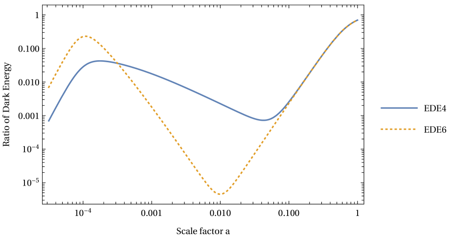
This approach is limited due to the resultant modification to the Silk damping scale, i.e., the photon diffusion scale Knox:2019rjx . One way to see the first problem is the fact that, as mentioned above, the phase shift and damping of the amplitude of high- peaks cannot be well recovered by changing only the dark matter and baryon density111For a scenario free from this diffusion problem, see Refs. Sekiguchi:2020teg ; Sekiguchi:2020igz .. For EDE models, a poor fit to large-scale structure data has also been claimed Hill:2020osr ; Ivanov:2020ril , which can be seen in the value of in Ref. Poulin:2018cxd . Despite this limitation, the introduction of extra radiation or EDE is a simple extension of CDM that addresses the discrepancy. The extra radiation energy and EDE contribute differently throughout the whole cosmological history. While EDE significantly contributes to the energy budget only around the epoch of matter-radiation equality to recombination and its energy density decreases quickly, the extra radiation exists throughout the whole history of the Universe. This difference can be seen in its effects on big bang nucleosystheisis (BBN). In fact, a study for with referring BBN in the context of the Hubble tension was done in Refs. Cuceu:2019for ; Schoneberg:2019wmt . In EDE models, although the negligible energy density of the EDE component at the BBN epoch appears not to change the BBN prediction, the baryon abundance inferred from the CMB would be different from that in the CDM model to adjust the CMB spectrum and hence the resultant light element abundance could be affected. In this paper, by taking the fit with BBN into account, we evaluate and compare these scenarios of additional relativistic degrees of freedoms and EDE.
This paper is organized as follows. In the next section, we first describe our modeling of the extra radiation and EDE. After we describe the methods and data sets used in our analysis in Sec. III, we show the results and discuss their interpretation in Sec. IV. The last section is devoted to a summary.
II Modeling
The expansion rate of the Universe—the Hubble parameter,—is defined as
| (3) |
where is the scale factor and a dot denotes a derivative with respect to cosmic time . In the following, we use the scale factor instead of time as a “time” variable. Then, we regard the Hubble parameter as a function of , and normalize the scale factor as , with being the age of the Universe.
II.1 Extra radiation
One simple “solution” to the Hubble tension is to increase the effective number of neutrinos , which is expressed as
| (4) |
Here,
| (5) |
with being the reduced Planck mass, are the present values of the density parameters for species. and stand for CMB photons and neutrinos, respectively. In the following, we call this an model.
II.2 Early dark energy
In the literature, the EDE scenarios are modeled by a variety of functional forms for scalar fields, such as axion-potential-like Poulin:2018zxs ; Poulin:2018dzj ; Poulin:2018cxd , polynomial Agrawal:2019lmo , acoustic dark energy Lin:2019qug , -attractor-like Braglia:2020bym , and others. Those properties and differences due to various potential forms have been studied in those literatures. In contrast, in this work, since our main focus is on the differences between the EDE and the extra radiation, we adopt a simple fluid picture. In order to treat time-dependent dark energy, we define the dark energy equation of state . By integrating the continuity equation
| (6) |
we obtain Copeland:2006wr
| (7) |
We find the cosmic expansion by solving the Friedman equation for the EDE models
| (8) | ||||
| (9) |
The indices of each parameter, , stand for cold dark matter, baryons, radiation, and dark energy, respectively. Here, DE represents the sum of the EDE component and the cosmological constant which is responsible for the present accelerating cosmic expansion as .
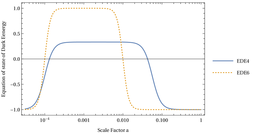
In the EDE scenarios, the energy component of dark energy becomes significant around the moment of the matter-radiation equality and contributes to about several percents of the total energy density. Soon after that moment, the EDE component decreases as and faster than the background energy densities do. Here we introduce two parameters: and . is the scale factor at the moment when the EDE starts to decrease like radiation or kination . is the scale factor at the moment when the EDE component becomes as small as the cosmological constant. Phenomenologically, we parametrize the equation of state as
| (10) |
and the resultant parameter is given by
| (11) |
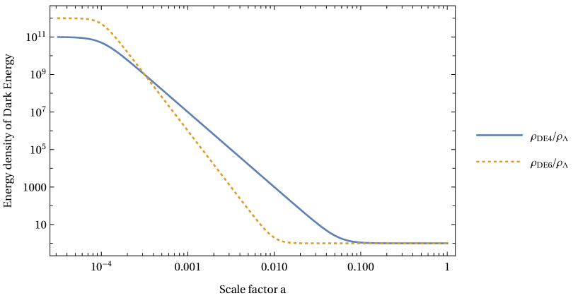
For and , the dark energy behaves like a cosmological constant. Typical evolutions of and normalized by are shown in Fig. 1. We note that the above is proportional to the parameter often used in literature as
| (12) |
Typical evolutions of are shown in Fig. 2.
Dealing perturbation, in this work we set its effective sound speed for perturbations of the EDE component, motivated by a class of scalar field models. One may compare this to each specific scalar potential model in e.g., Refs. Poulin:2018zxs ; Poulin:2018dzj ; Poulin:2018cxd ; Alexander:2019rsc ; Braglia:2020bym ; Murgia:2020ryi ; Chudaykin:2020acu ; Chudaykin:2020igl . Our modeling will be closer to nonoscillatory scalar field models Lin:2019qug ; Braglia:2020bym .
III Data and Analysis
We perform a Markov Chain Monte Carlo (MCMC) analysis on an model and the EDE model described in the previous section. We use the public MCMC code CosmoMC-planck2018 Lewis:2002ah and implement the above EDE scenarios by modifying its equation file in CAMB. For estimation of light elements, we use PArthENoPE standard Pisanti:2007hk in CosmoMC.
III.1 Data sets
We analyze models using the following cosmological observation data sets. We include both temperature and polarization likelihoods for high ( to in TT and to in EE and TE) and low Commander and lowE SimAll ( to ) of Planck (2018) measurement of the CMB temperature anisotropy Aghanim:2018eyx . We also include Planck lensing data Aghanim:2018oex . For constraints on low-redshift cosmology, we include BAO data from 6dF Beutler:2011hx , DR7 Ross:2014qpa , and DR12 Alam:2016hwk . We also include Pantheon data Scolnic:2017caz on the local measurement of light curves and luminosity distance of supernovae, as well as SH0ES (R19) data Riess:2019cxk on the local measurement of the Hubble constant from the Hubble Space Telescope’s observation of Supernovae and Cephied variables. Finally, we include the data sets on the helium mass fraction Aver:2015iza and deuterium abundance D/H Cooke:2017cwo to impose the constraints from BBN.
III.2 EDE and neutrino parameter sets
We take a prior range of . This is motivated by the limit (BBN++D/H,) in Ref. Cyburt:2015mya .
For the EDE model with , which is denoted as EDE hereafter, we fix and vary parameters in the range . For the EDE model with , which is denoted as EDE hereafter, we fix and vary parameters in the range . These values of are motivated by the results in Ref. Poulin:2018cxd .
IV Result and discussion
IV.1 Result
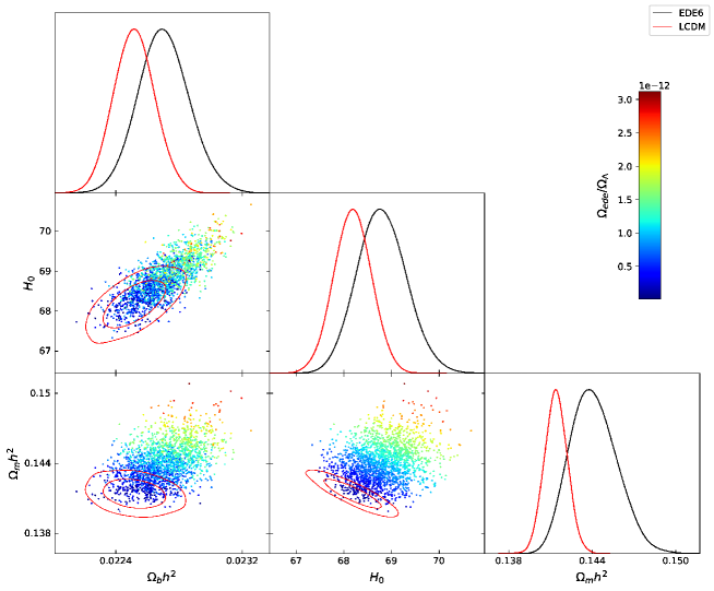
Although we have examined both the EDE and EDE models, we have confirmed that the EDE model gives a slightly better fit than the EDE model, as has been pointed out in previous works. Thus, we show a posterior distribution for only the EDE model in Fig. 4 and the posterior distribution for an model in Fig. 4. In addition to the above two models which have been studied in literature, we also consider the model where both the extra radiation and EDE components exist, which hereafter we call the coexisting model or EDE, motivated by the fact that these are in principle independent sectors.
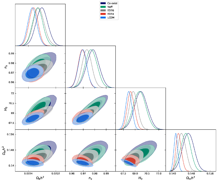
To compare models, we show the combined plots of the EDE, the EDE, the coexistence model with EDE plus , and together with CDM for reference in Fig. 6. These results are also summarized in Table 1. It is clear that both the EDE and coexistence models prefer a larger value of than other models. We confirm that the EDE model shows the poorest improvement for the tension, as shown in Fig. 6.
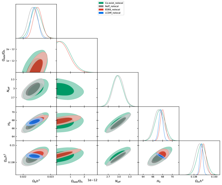
For reference, we also show the same plot of the analysis without including Pantheon and R19 data [in other words (CMBBAOBBN)] in Fig. 6, because one may wonder used data sets dependence. One can confirm that the results for in Fig. 6 almost reproduce Fig. 35 in Ref. Aghanim:2018eyx . The constraints on EDE in Figs. 6 and 6 do not differ significantly. On the other hand, we can find sizable shifts of the posterior and the cental values for and the coexintence model, depending on whether we include R19 data. If one pays attention to only the central values, it looks like the EDE indicates the largest value of and models with indicate even smaller values than CDM does. However, the constraints of a certain confidence level on the and the coexistence models are much weaker than those for the EDE model. In addition, one should be aware of the presence of the prior dependence in Fig. 6, where the energy density of EDE is positive definite, while we allow for the models with .
| Model | EDE | EDE+ | CDM | |
|---|---|---|---|---|
| CDM | CDM | |||
| 3.046 | 3.046 | |||
| [km/s/Mpc] | ||||
| CMB:lensing | 8.83 | 8.81 | 8.52 | 9.17 |
| CMB:TTTEEE | 2350.05 | 2352 | 2348.86 | 2354.72 |
| CMB:low | 22.04 | 21.48 | 22.83 | 21.93 |
| CMB:lowE | 395.88 | 397.82 | 399.52 | 396.51 |
| Cooke | 0.65 | 0.18 | 0.30 | 0.0037 |
| Aver | 0.23 | 0.92 | 0.22 | 1.56 |
| SH0ES | 15.18 | 10.56 | 16.75 | 10.71 |
| JLA Pantheon18 | 1034.85 | 1034.74 | 1034.77 | 1034.77 |
| BAO | 5.35 | 5.41 | 5.24 | 5.32 |
| prior | 5.89 | 3.71 | 4.51 | 3.30 |
| total | 3838.95 | 3835.63 | 3841.52 | 3838.00 |
IV.2 Discussions
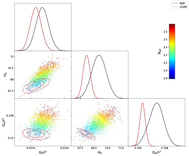
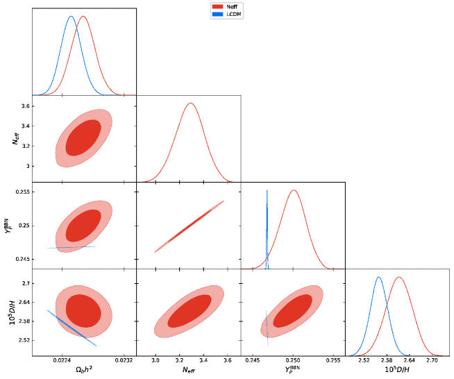
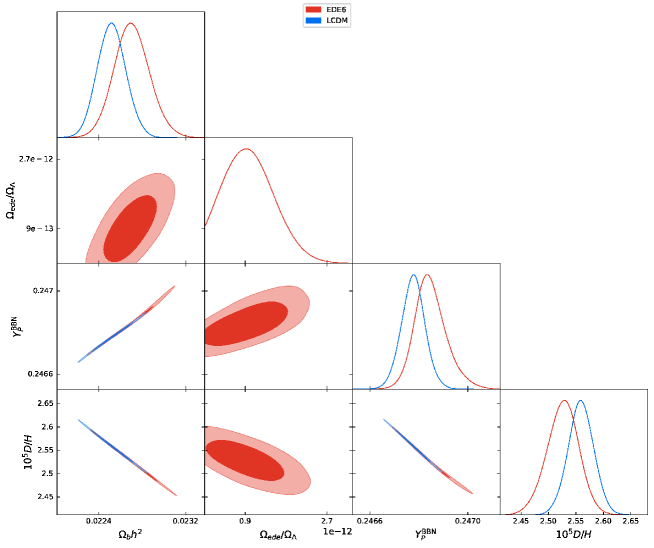
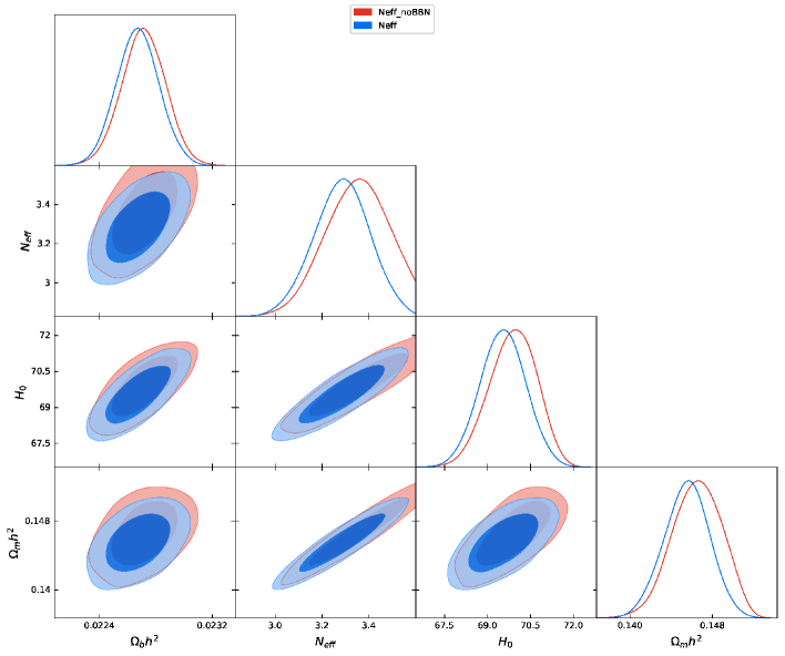
As is well known, an increase of affects the fit with the observations of light elements, because it contributes the cosmic expansion at the BBN epoch and alters the ratio. This leads to an increase in both the helium mass fraction and deuterium abundance D/H. By increasing , the CMB fit simultaneously indicates a larger which reduces D/H. In total, the enhancement of D/H is suppressed. As a result, the of observations () increases, while the of D/H observations () increases a little. In fact, the value of of the model is smaller than that in the CDM model. This can be seen in Fig. 7 and Table 1. On the other hand, in the EDE scenarios, increasing to adjust the CMB fit reduces the D/H abundance significantly. Thus, increases a little, while increases. This can be seen in Fig. 8 and Table 1. The tradeoff relation between the fit to the helium mass fraction and deuterium abundance D/H can be seen more clearly in Table 1, where we compare it with the coexistence model.
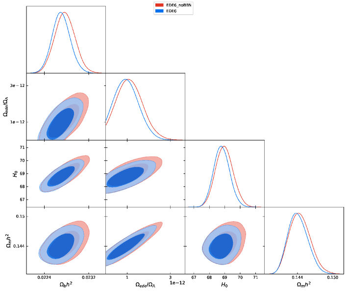
The constraint on from BBN and BAO data only without including CMB or SH0SE data has been derived as , which is less than Cyburt:2015mya . As is well known, a larger is disfavored by BBN. This is consistent with the results in Table 1. What we additionally find is that the EDE models without are also limited by BBN, because they predicts too little D/H abundance by too large .
In the literature on the new physics interpretation of the Hubble tension, data sets have not included BBN data. We have derived constraints from the data sets with and without BBN data for each model. As can be expected, data sets without BBN indicate larger values of and . The magnitudes of the differences are shown in Fig. 9.
V Summary
A shorter sound horizon scale at the recombination epoch, arising from introducing extra energy components such as extra radiation or EDE is a simple approach to resolving the so-called Hubble tension. However, then the compatibility with successful BBN would be a concern, because the extra radiation may contribute to the cosmic expansion or the inferred baryon asymmetry would be different from that in the CDM. We have compared the EDE models, model, and a coexistence model, paying attention to the fit to BBN. In fact, the EDE models are also subject to the BBN constraints by increasing the order-unity as in the model. Our main results are summarized in Fig. 6 and Table 1. By comparing the posteriors based on the CMBBAOPantheonR19 combined data, both the and a coexistence models indicate the largest between all of the models studied. can be as large as km/s/Mpc within only for the coexistence model. The goodness of the fits for the models in terms of are also listed in Table 1. The fitting is good in the order of the EDE, , and EDE models and the CDM. The difference of the best-fit values between the EDE and models is tiny, while the difference is about . The extra radiation seems to be more effective at causing a large than the EDE model. Thus, the model is a much simpler and better model than the EDE models.
We also examined the data sets dependence, whether we include BBN or not. The difference on in the model is only about in its mean value, however, the including errors indicate
| (14) | |||
| (15) |
and there is almost difference in the upper. By comparing this with Eq. (1), we can see the impact of the R data compared to the R data. For EDE models, if we include the BBN data, a smaller and smaller EDE energy density are preferred.
Acknowledgments
We would like to thank T. Sekiguchi for kind correspondences concerning the use of CosmoMC. This work is supported in part by the Japan Society for the Promotion of Science (JSPS) KAKENHI Grants Nos. 19K03860, 19H05091, and 19K03865 (O.S.).
References
- (1) N. Aghanim et al. (Planck Collaboration), Astron. Astrophys. 641, A6 (2020).
- (2) A. G. Riess et al., Astrophys. J. 855, 136 (2018).
- (3) A. G. Riess, S. Casertano, W. Yuan, L. M. Macri and D. Scolnic, Astrophys. J. 876, 85 (2019).
- (4) K. C. Wong et al., Mon. Not. R. Astron. Soc. 498. 1420 (2020).
- (5) G. Efstathiou, Mon. Not. R. Astron. Soc. 440, 1138 (2014).
- (6) W. L. Freedman, Nat. Astron. 1, 0121 (2017).
- (7) M. Rameez and S. Sarkar, [arXiv:1911.06456 [astro-ph.CO]].
- (8) M. M. Ivanov, Y. Ali-Haï¿œmoud, and J. Lesgourgues, Phys. Rev. D 102, 063515 (2020).
- (9) J. L. Bernal, L. Verde and A. G. Riess, J. Cosmol. Astropart. Phys. 10 (2016) 019.
- (10) K. Aylor, M. Joy, L. Knox, M. Millea, S. Raghunathan and W. L. K. Wu, Astrophys. J. 874, 4 (2019).
- (11) F. D’Eramo, R. Z. Ferreira, A. Notari and J. L. Bernal, J. Cosmol. Astropart. Phys. 11 (2018) 014.
- (12) M. Escudero, D. Hooper, G. Krnjaic and M. Pierre, J. High Energy. Phys. 03 (2019) 071.
- (13) M. Escudero and S. J. Witte, Eur. Phys. J. C 80, 294 (2020).
- (14) N. Okada and O. Seto, Phys. Rev. D 101, 023522 (2020).
- (15) V. Poulin, K. K. Boddy, S. Bird and M. Kamionkowski, Phys. Rev. D 97 123504 (2018).
- (16) V. Poulin, T. L. Smith, D. Grin, T. Karwal and M. Kamionkowski, Phys. Rev. D 98, 083525 (2018).
- (17) V. Poulin, T. L. Smith, T. Karwal and M. Kamionkowski, Phys. Rev. Lett. 122, 221301 (2019).
- (18) P. Agrawal, F. Y. Cyr-Racine, D. Pinner and L. Randall, [arXiv:1904.01016].
- (19) S. Alexander and E. McDonough, Phys. Lett. B 797, 134830 (2019).
- (20) M. X. Lin, G. Benevento, W. Hu and M. Raveri, Phys. Rev. D 100, 063542 (2019).
- (21) T. L. Smith, V. Poulin and M. A. Amin, Phys. Rev. D 101, 063523 (2020).
- (22) K. V. Berghaus and T. Karwal, Phys. Rev. D 101, 083537 (2020).
- (23) J. Sakstein and M. Trodden, Phys. Rev. Lett. 124, 161301 (2020).
- (24) A. Chudaykin, D. Gorbunov and N. Nedelko, J. Cosmol. Astropart. Phys. 08 (2020) 013.
- (25) M. Braglia, W. T. Emond, F. Finelli, A. E. Gumrukcuoglu and K. Koyama, Phys. Rev. D 102, 083513 (2020).
- (26) F. Niedermann and M. S. Sloth, Phys. Rev. D 102, 063527 (2020).
- (27) M. Gonzalez, M. P. Hertzberg and F. Rompineve, J. Cosmol. Astropart. Phys. 10 (2020) 028.
- (28) M. X. Lin, W. Hu and M. Raveri, Phys. Rev. D 102, 123523 (2020).
- (29) R. Murgia, G. F. Abellï¿œn and V. Poulin, Phys. Rev. D 103, 063502 (2021).
- (30) A. Chudaykin, D. Gorbunov and N. Nedelko, Phys. Rev. D 103, 043529 (2021).
- (31) L. Yin, [arXiv:2012.13917].
- (32) W. Hu and S. Dodelson, Ann. Rev. Astron. Astrophys. 40, 171 (2002).
- (33) L. Knox and M. Millea, Phys. Rev. D 101, 043533 (2020).
- (34) T. Sekiguchi and T. Takahashi, Phys. Rev. D 103. 083507 (2021)
- (35) T. Sekiguchi and T. Takahashi, Phys. Rev. D 103. 083516 (2021)
- (36) J. C. Hill, E. McDonough, M. W. Toomey and S. Alexander, Phys. Rev. D 102, 043507 (2020).
- (37) M. M. Ivanov, E. McDonough, J. C. Hill, M. Simonović, M. W. Toomey, S. Alexander and M. Zaldarriaga, Phys. Rev. D 102, 103502 (2020).
- (38) A. Cuceu, J. Farr, P. Lemos and A. Font-Ribera, J. Cosmol. Astropart. Phys. 10 (2019) 044.
- (39) N. Schï¿œneberg, J. Lesgourgues and D. C. Hooper, J. Cosmol. Astropart. Phys. 10 (2019) 029.
- (40) E. J. Copeland, M. Sami and S. Tsujikawa, Int. J. Mod. Phys. D 15, 1753 (2006).
- (41) A. Lewis and S. Bridle, Phys. Rev. D 66, 103511 (2002).
- (42) O. Pisanti, A. Cirillo, S. Esposito, F. Iocco, G. Mangano, G. Miele and P. D. Serpico, Comput. Phys. Commun. 178, 956 (2008)
- (43) N. Aghanim et al. (Planck Collaboration), Astron. Astrophys. 641, A8 (2020).
- (44) F. Beutler, C. Blake, M. Colless, D. H. Jones, L. Staveley-Smith, L. Campbell, Q. Parker, W. Saunders and F. Watson, Mon. Not. R. Astron. Soc. 416, 3017 (2011).
- (45) A. J. Ross, L. Samushia, C. Howlett, W. J. Percival, A. Burden and M. Manera, Mon. Not. R. Astron. Soc. 449, 835 (2015).
- (46) S. Alam et al. (BOSS Collaboration), Mon. Not. R. Astron. Soc. 470, 2617 (2017).
- (47) D. M. Scolnic, D. O. Jones, A. Rest, Y. C. Pan, R. Chornock, R. J. Foley, M. E. Huber, R. Kessler, G. Narayan, A. G. Riess et al., Astrophys. J. 859, 101 (2018).
- (48) E. Aver, K. A. Olive and E. D. Skillman, J. Cosmol. Astropart. Phys. 07 (2015) 011.
- (49) R. J. Cooke, M. Pettini and C. C. Steidel, Astrophys. J. 855, 102 (2018).
- (50) R. H. Cyburt, B. D. Fields, K. A. Olive and T. H. Yeh, Rev. Mod. Phys. 88, 015004 (2016).