Comparison of multi-mode Hong-Ou-Mandel interference and multi-slit interference

Since its discovery in 1987, the Hong-Ou-Mandel (HOM) interference using downconverted biphotons has shown a wide variety of applications in quantum optics [1, 2, 3, 4, 5]. In traditional HOM interference, the biphotons are usually correlated in one discrete spectral mode. However, the biphotons involved can be correlated in multiple discrete spectral modes, and this two-body high-dimensional entangled state can be called entangled qudits [6, 7, 8, 9]. Here, we define the HOM interference using frequency entangled qudits as the multi-mode HOM interference (MM-HOMI). One important characteristic of MM-HOMI is that its interference patterns are significantly narrower than those in single-mode HOM interference. Such narrow interference fringes provide more Fisher information in phase estimation [10, 11, 12, 13, 14, 15]. As a result, MM-HOMI is very promising in quantum metrology.

Recently, many works have been devoted to the study of HOM interference using biphotons in multi-frequency modes. Lingaraju et al. investigated the effect of spectral phase coherence of multi-frequency modes in HOM interference [13]. Chen et al. utilized HOM interference as a tool to characterize up to six-mode frequency entangled qudits [14, 15]. Morrison et al. prepared an eight-mode frequency entangled state in a customized poling crystal and tested its HOM interference patterns [16]. In addition, HOM interference using biphoton frequency combs, which have a large number of discrete frequency modes, has also been widely investigated [17, 18, 19, 20].

However, as the mode number increases, the MM-HOMI pattern becomes more and more complicated, which makes it challenging to understand intuitively. To address this issue, we first present the theory and simulation of MM-HOMI and then compare it with a well-known classical interference, the multi-slit interference (MSI)[21, 22, 23, 24, 25]. We demonstrate that the MM-HOMI and the MSI exhibit a strong mapping relationship.

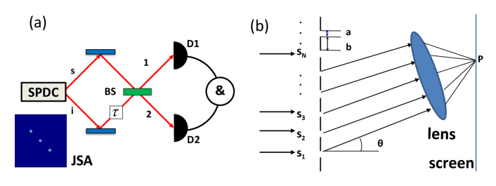
The typical setup for HOM interference is shown in Fig. 1 (a). The signal and idler photons generated from a spontaneous parametric downconversion (SPDC) process can be expressed as [26, 27, 28]

$$|\psi\rangle=\iint\nolimits_{-\infty}^{+\infty}d{\omega_{s}}d{\omega_{i}}f\left(\omega_{s},\omega_{i}\right)\hat{a}_{s}^{\dagger}\left(\omega_{s}\right)\hat{a}_{i}^{\dagger}\left(\omega_{i}\right)|0\rangle|0\rangle,$$

(1)

where $f\left(\omega_{s},\omega_{i}\right)$ is the biphoton’s joint spectral amplitude (JSA), $\omega$ is the angular frequency, and ${\hat{a}^{\dagger}}$ is the creation operator. The subscripts $s$ and $i$ represent the signal and idler photons, respectively. In a HOM interference, the two-photon coincidence probability $P\left(\tau\right)$ can be written as [29, 30]

$$\begin{array}[]{lll}P\left(\tau\right)=\frac{1}{2}-\frac{1}{2}\iint\nolimits_{-\infty}^{+\infty}d{\omega_{1}}d{\omega_{2}}{\left|f\left({{\omega_{1}},{\omega_{2}}}\right)\right|^{2}}{\cos\left(\left({{\omega_{1}}-{\omega_{2}}}\right)\tau\right)},\end{array}$$

(2)

where $\omega_{1}$ and $\omega_{2}$ are the frequencies detected by detectors D1 and D2 in Fig. 1 (a). For simplicity, in the above equation, we have assumed that $f\left(\omega_{1},\omega_{2}\right)$ is normalized and satisfies the exchanging symmetry of $f\left(\omega_{1},\omega_{2}\right)=f\left(\omega_{2},\omega_{1}\right)$. See the Appendix for more details.

In the MM-HOMI, the JSA can be written as:

$$\begin{array}[]{l}f\left({{\omega_{1}},{\omega_{2}}}\right)=\sum\limits_{k=1}^{N}{{f_{0}}\left({{\omega_{1}}-{\omega_{0}}-\left({2k-N-1}\right)\alpha,{\omega_{2}}-{\omega_{0}}+\left({2k-N-1}\right)\alpha}\right)},\\ \end{array}$$

(3)

where $f_{0}\left({\omega_{1}},{\omega_{2}}\right)$ is an arbitrary distribution function of the single spectral mode, $N$ is the mode number, $\alpha$ represents the mode spacing, and $\omega_{0}$ is the mode’s central frequency. As calculated in the Appendix, $P\left(\tau\right)$ can be simplified as

$$\begin{array}[]{lll}P\left(\tau\right)&=\frac{1}{2}\left[1-\frac{1}{{N}}\frac{{\sin(2N\alpha\tau)}}{{\sin(2\alpha\tau)}}\iint\nolimits_{-\infty}^{\infty}{d{\omega_{1}}}d{\omega_{2}}{f_{0}}^{2}\left({{\omega_{1}},{\omega_{2}}}\right)\cos\left({\left({{\omega_{1}}-{\omega_{2}}}\right)\tau}\right)\right]\\ &=\frac{1}{2}\left[1-P_{0}\frac{{{\rm{\sin}}\left({Nx}\right)}}{{{\rm{\sin}}\left({x}\right)}}\right],\\ \end{array}$$

(4)

where $x=2\alpha\tau$, which corresponds to the phase spacing caused by two adjacent spectral modes. $P_{0}=\frac{1}{{N}}\iint\nolimits_{-\infty}^{\infty}{d{\omega_{1}}}d{\omega_{2}}{f_{0}}^{2}\left({{\omega_{1}},{\omega_{2}}}\right)\cos\left({\left({{\omega_{1}}-{\omega_{2}}}\right)\tau}\right)$ corresponds to the envelope of the interference patterns.

We can observe in Eq. (4) that the MM-HOMI is determined by two factors: the envelope factor $P_{0}$ and the details factor $\frac{{{\rm{\sin}}\left({Nx}\right)}}{{{\rm{\sin}}\left({x}\right)}}$. $P_{0}$ is contributed by the single-mode HOM interference (for N=1). $P_{0}$ can also be expressed in the form of a Fourier transformation by projecting ${f_{0}}^{2}\left({{\omega_{1}},{\omega_{2}}}\right)$ on the axis of $\omega_{1}-\omega_{2}$, as shown in Eq. (23) in the Appendix.

For simplicity, we can set $\;f\left({{\omega_{1}},{\omega_{2}}}\right)$ to a multi-mode Gaussian distribution[16, 31]:

$$\begin{array}[]{l}f\left({{\omega_{1}},{\omega_{2}}}\right)=\mathop{\sum}\limits_{k=1}^{N}\exp\left[-\frac{{{{({\omega_{1}}-{\omega_{0}}-\left({2k-N-1}\right)\alpha)}^{2}}}}{{{\gamma^{2}}}}-\frac{{{{({\omega_{2}}-{\omega_{0}}+\left({2k-N-1}\right)\alpha)}^{2}}}}{{{\gamma^{2}}}}\right],\\ \end{array}$$

(5)

where $N$ is the mode number, $\gamma$ represents the mode width. In a real experiment, $\gamma$ and $\alpha$ are determined by the width of the pump and the phase-matching function of the crystal [16]. As calculated in the Appendix, $P_{0}\left(\tau\right)$ can be simplified as

$$\begin{array}[]{lll}P_{0}=\frac{1}{{N}}\exp\left(-\frac{{{\gamma^{2}}{\tau^{2}}}}{4}\right).\end{array}$$

(6)

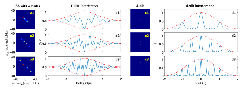
According to Eq. (4), Eq. (5) and Eq. (6), we can plot the interference patterns of MM-HOMI. As shown in Fig. 2, the first column is the JSA of the biphotons, and the mode number is 1, 3, 5, 7, 2, 4, 6, and 8. Here, we choose the unit ellipticity for each mode, since this is the simplest case and has been realized in experiment [16]. The second column is the corresponding MM-HOMI pattern.

Firstly, we compare the envelopes of the interference patterns. The odd-number MM-HOMI patterns have an asymmetric envelope, whereas the even-number MM-HOMI patterns are symmetric to the line of $P\left(\tau\right)=0.5$. This is due to the characteristics of the function $\frac{\sin\left(Nx\right)}{\sin\left(x\right)}$, which is asymmetric (symmetric) when N is an odd (even) number.

Secondly, we compare the primary and secondary valley (peak) numbers. For the odd-number MM-HOMI patterns, there are (N-3)/2 secondary valleys (for N$>$3) between two primary valleys, while for the even-number MM-HOMI patterns, there are N-2 secondary valleys (for N$>$2) between two primary valleys.

So far, we have analyzed the properties of the MM-HOMI. However, we can notice that the interference patterns in Fig. 2 are very complicated. One might gain some insight by comparing MM-HOMI with a classical well-known multi-slit interference (MSI). It may be intuitive to understand that the multiple spectra function in a manner similar to the multiple slits.

Next, we deduce the mathematical form of MSI and compare it with MM-HOMI.

The typical setup for MSI is shown in Fig. 1 (b). Here, the number of slits is $N$, the slit width is $a$, the interval of the slits is $b$, and $a+b=d$. As calculated in the Appendix, the amplitude of the diffraction pattern at point $p$ is

$$\begin{array}[]{lll}A_{p}={A_{0}}\frac{{\sin\left(u\right)}}{u}\frac{{\sin\left(Nv\right)}}{{\sin\left(v\right)}},\end{array}$$

(7)

where $A_{0}$ is a constant determined by the power of the light source, the distance between the slit and the screen, and the size of the slit [21]. $u=\frac{{\pi a\sin\theta}}{\lambda}$ represents the phase difference in one slit. $v=\frac{{\pi d\sin\theta}}{\lambda}$ represents the phase difference between two adjacent slits. $\lambda$ is the wavelength of the input light and $\theta$ is the tilt angle of the light, as shown in Fig. 1 (b). For simplicity, we can set $A_{0}=1$. The intensity of the diffraction pattern is:

$$\begin{array}[]{lll}I={\mid A_{p}\mid}^{2}=\left(\frac{\sin\left(u\right)}{u}\right)^{2}\left(\frac{\sin\left(Nv\right)}{\sin\left(v\right)}\right)^{2}=I_{0}\left(\frac{\sin\left(Nv\right)}{\sin\left(v\right)}\right)^{2},\\ \end{array}$$

(8)

where ${I_{0}}=\left(\frac{{\sin}{\left(u\right)}}{u}\right)^{2}$ is the intensity due to one-slit diffraction, which is also the interference pattern’s envelope.

According to Eq. (8), we can plot the interference patterns of MSI, as shown in the third and fourth columns in Fig. 2. The parameters are listed in detail in the caption of Fig. 2. There are N-2 secondary peaks (for N$>$2) between two primary peaks in the fourth column of Fig. 2. This is comparable to the even-number MM-HOMI patterns, which also have N-2 secondary valleys (for N$>$2) between two primary valleys.

Next, we investigate the influence of the mode size in MM-HOMI and MSI. Figure 3 (a1-a3, b1-b3) displays the JSA of the biphotons and the corresponding MM-HOMI. Here, we set $\alpha$ to be fixed at 5 rad$\cdot$THz, and $\gamma$ to be 0.5 rad$\cdot$THz, 2.5 rad$\cdot$THz, and 4.5 rad$\cdot$THz, respectively. It can be observed that with the increase of $\gamma$, the envelope becomes narrower, but the spacing of adjacent peaks (valleys) does not change. This phenomenon can be well explained by Eq. (4). Figure 3 (c1-c3, d1-d3) shows the 4-slit distributions and the corresponding MSI. It can be noticed that the envelope also becomes narrower with the increase of $a$, which is similar to the phenomenon of MM-HOMI.

Then, let us examine the impact of mode spacing on MM-HOMI and MSI. Figure 4 (a1-a3, b1-b3) depicts the JSA and MM-HOMI of biphotons with $\gamma$ fixed at 2 rad$\cdot$THz and $\alpha$ increasing from 2.5 rad$\cdot$THz to 5 rad$\cdot$THz and 7.5 rad$\cdot$THz. Figure 4 (c1-c3, d1-d3) shows the slit distributions and the corresponding MSI. By comparing (a1-b3) with (c1-d3), we can observe that the envelope remains constant, while the number of peaks and valleys increases as mode spacing increases. These phenomena can also be well explained by Eq. (4) and Eq. (8).

After analyzing Figs. (4, 5, 6) and Eqs. (4, 8), we can confirm that the MM-HOMI and MSI have a strong mapping relationship, as summarized in Tab. 1. The phase variable $x$, which accumulates in the time domain, represents the phase spacing between two spectra modes in the MM-HOMI; while the phase variable $v$, which accumulates in the space domain, represents the phase spacing between two slits in the MSI. Both MM-HOMI and MSI are determined by two factors: the envelope factor and the details factor. The details factor includes a common term of $\frac{{{\rm{\sin}}\left({Nx}\right)}}{{{\rm{\sin}}\left({x}\right)}}$ with a mode number of $N$. In MM-HOMI, the envelope factor $P_{0}$ corresponds to the HOM interference of a single spectral mode, and $P_{0}$ is also related to the Fourier transform of a single spectral mode, as shown in Eq. (23). Similarly, the details factor $I_{0}$ corresponds to the single-slit diffraction, and it is also contributed by the Fourier transform of a single slit, as explained in Eq. (28) in the Appendix. Therefore, we can conclude that the multiple spectra indeed function similarly to the multiple slits, as we expected at the beginning of this section. Consequently, the mapping relationship really can help on the intuitive understanding of the MM-HOMI.

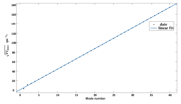
MSI has numerous applications in optical measurement, with one typical example being the diffraction-grating-based spectrometer. The resolving power of a diffraction grating is proportional to the total number of slits (or grooves) on the grating [21, 22, 23, 24, 25]. Inspired by this feature, here we consider the resolving power of a MM-HOMI in quantum metrology by increasing the total number of the spectral modes.

The ultimate limit on the precision of time estimation is the Cramér-Rao bound [12, 32] , which states that the variance of any unbiased estimator is bounded by

$$Var(\tilde{t})\geq\frac{1}{{Num\times FI}},$$

(9)

where $\tilde{t}$ is the estimator of time $t$, and $Num$ is the number of measurement times and $FI$ is the Fisher information (FI). For a single measurement, $Num$=1. So, the standard deviation (SD) is bound by

$$SD(\tilde{t})\geq\frac{1}{{\sqrt{FI}}}.$$

(10)

FI of a single interference fringe can be calculated as [10, 33]:

$$FI\left(\tau\right)=P\left(\tau\right)\left({\frac{{\partial\left[\ln P\left(\tau\right)\right]}}{{\partial\tau}}}\right)^{2}+\left[1-P\left(\tau\right)\right]\left({\frac{{\partial\left[\ln\left(1-P\left(\tau\right)\right)\right]}}{{\partial\tau}}}\right)^{2}=\frac{\left[{P^{\prime}\left(\tau\right)}\right]^{2}}{{P\left(\tau\right)\left[1-P\left(\tau\right)\right]}}.$$

(11)

By using Eq.(4) and Eq.(11), we can obtain the Fisher information of MM-HOMI as

$$\begin{array}[]{lll}FI\left(\tau\right)=\frac{{{{\left({\frac{{{\gamma^{2}}\tau}}{2}\sin\left({2\alpha N\tau}\right)-2\alpha N\cos\left({2\alpha N\tau}\right)+2\alpha\sin\left({2\alpha N\tau}\right)\cot\left({2\alpha\tau}\right)}\right)}^{2}}}}{{{N^{2}}\exp[\frac{{{\gamma^{2}}{\tau^{2}}}}{2}]{{\sin}^{2}}\left({2\alpha\tau}\right)-{{\sin}^{2}}\left({2\alpha N\tau}\right)}}.\end{array}$$

(12)

Figure 5(a1-a8) displays the simulated FI of the $P\left(\tau\right)$ in Fig. 2(b1-b8), with the mode number N increasing from 1 to 8. The single valley in Fig. 2(b8) is transferred to a double peak in Fig. 5(a8). Figure 6 summarizes the square root of maximal FI as a function of the mode number N ranging from 1 to 40. It is evident that the square root of maximal FI increases linearly with the increase in mode number. This suggests that increasing the mode number is a powerful method to improve precision in time or phase estimation.

From the viewpoint of the extended Wiener-Khinchin theorem (e-WKT) [30], the Fourier transform of the HOM interference pattern is determined by the difference–frequency distribution of the JSI, i.e., the projection of $f\left({{\omega_{1}},{\omega_{2}}}\right)$ onto the $\omega_{1}-\omega_{2}$ axis. The e-WKT is not only applicable to the single-mode case but also explains the multi-mode case in this study. Specifically, the interference patterns of MM-HOMI are determined by the Fourier transform of the difference–frequency distribution of the multi-mode JSI.

To gain a deeper understanding of the multi-mode effect, we also compared the MM-HOMI and MSI with two other important interferences in quantum optics: the multi-mode Mach–Zehnder interference (MM-MZI) and the multi-mode NOON state interference (MM-NOONSI), using the setups shown in Fig. 7 (a, b). Here, the NOON-state is a $(\left|{20}\right\rangle+\left|{02}\right\rangle)/\sqrt{2}$ state, which has a photon number of 2, but with a spectral-mode number of N, as shown in Fig. 7(e1-e8). As calculated in the Appendix, the single count in a MM-MZI can be expressed as

$$\begin{array}[]{l}P_{MZI}\left(\tau\right)=\frac{1}{2}+\frac{1}{{2N}}\exp\left[{-\frac{{{\gamma^{2}}{\tau^{2}}}}{8}}\right]\frac{{\sin\left({N\alpha\tau}\right)}}{{\sin\left({\alpha\tau}\right)}}\cos\left({{\omega_{0}}\tau}\right),\\ \end{array}$$

(13)

and the coincidence counts in a MM-NOONSI can be expressed as

$$\begin{array}[]{l}P_{NOON}\left(\tau\right)=\frac{1}{2}+\frac{1}{{2N}}\exp\left[-\frac{{{\gamma^{2}}{\tau^{2}}}}{4}\right]\frac{{\sin\left({2N\alpha\tau}\right)}}{{\sin\left({2\alpha\tau}\right)}}\cos\left({2{\omega_{0}}\tau}\right).\\ \end{array}$$

(14)

In the above two models, Gaussian envelopes were chosen for simplicity. Refer to the Appendix for deductions using arbitrary envelopes. The parameters are listed in detail in the caption of Fig. 7. By comparing the theoretical simulations in Fig. 7 (d1-d8) and (f1-f8), we observe that there are N-2 secondary peaks (for N $>$ 3) between the two main peaks in N-mode Mach–Zehnder interference and N-mode NOON-state interference.

By comparing Eq. (13), Eq. (14), Eq. (4), and Eq. (8), we observe that the MM-MZI and MM-NOONSI are also contributed by the details factor of $\sin\left(Nx\right)/\sin\left(x\right)$, but multiplied by a factor of $\cos\left(\omega_{0}\tau\right)$ or $\cos\left(2\omega_{0}\tau\right)$. In general, the connection between the MM-HOMI, the MSI, the MM-MZI, and the MM-NOONSI is that all these interferences are contributed by N input modes in physics and determined by the factor of $\sin\left(Nx\right)/\sin\left(x\right)$ in mathematics.

In conclusion, we have presented the theory and simulation of MM-HOMI and compared them with MSI. We confirm that both interferences are determined by two factors: the envelope factor and the details factor. For MM-HOMI (MSI), the envelope factor is determined by each mode (slit), while the details factor is determined by the N modes (slits). The mapping relationship between MM-HOMI and MSI may provide an intuitive explanation of MM-HOMI. As an example of its application, we demonstrate that the square root of maximal Fisher information in a MM-HOMI increases linearly with the increase of mode numbers, indicating that increasing the mode number is a potent method for enhancing precision in quantum metrology.

In this section, we deduce the equation of HOMI using a biphoton state with a multi-mode distribution. The joint spectral amplitude (JSA) of the biphoton state from an SPDC source can be expressed as$f\left(\omega_{s},\omega_{i}\right)$, and the input two-photon state is

$$\begin{array}[]{lll}\left|\psi\right\rangle=\iint_{-\infty}^{+\infty}{d\omega_{s}}d\omega_{i}f\left(\omega_{s},\omega_{i}\right){\hat{a}}_{s}^{\dagger}\left(\omega_{s}\right){\hat{a}}_{i}^{\dagger}\left(\omega_{i}\right)\left|00\right\rangle,\end{array}$$

(15)

where the subscripts $s$ and $i$ denote the signal and idler photons, respectively, and$\ {\hat{a}}^{\dagger}\left(\omega\right)$is the creation operator of the signal and idler photons at angular frequency $\omega$. The detection field operators of detector 1 (D1) and detector 2 (D2) are ${\hat{E}}_{1}^{\left(+\right)}\left(t_{1}\right)=\frac{1}{\sqrt{2\pi}}\int_{0}^{\infty}{d\omega_{1}{\hat{a}}_{1}\left(\omega_{1}\right)e^{-i{\omega_{1}}{}t_{1}}}$ and $\hat{E}_{2}^{\left(+\right)}\left(t_{2}\right)=\frac{1}{\sqrt{2\pi}}\int_{0}^{\infty}{d\omega_{2}{\hat{a}}_{2}\left(\omega_{2}\right)e^{-i\omega_{2}t_{2}}}$, where subscripts 1 and 2 denote the photons detected by $D1$ and $D2$, respectively. The transformation rule of a 50/50 beam splitter (BS) after a delay time $\tau$ is ${\hat{a}}_{1}\left(\omega_{1}\right)=\frac{1}{\sqrt{2}}\left[{\hat{a}}_{s}\left(\omega_{1}\right)+{\hat{a}}_{i}\left(\omega_{1}\right)e^{-i\omega_{1}\tau}\right]$ and ${\hat{a}}_{2}\left(\omega_{2}\right)=\frac{1}{\sqrt{2}}\left[{\hat{a}}_{s}\left(\omega_{2}\right)+{\hat{a}}_{i}\left(\omega_{2}\right)e^{-i\omega_{2}\tau}\right]$. So, we can rewrite the field operators as

$$\begin{array}[]{lll}{\hat{E}}_{1}^{\left(+\right)}\left(t_{1}\right)=\frac{1}{\sqrt{4\pi}}\int_{-\infty}^{+\infty}{d\omega_{1}}\left[{\hat{a}}_{s}\left(\omega_{1}\right)e^{-i\omega_{1}t_{1}}+{\hat{a}}_{i}\left(\omega_{1}\right)e^{-i\omega_{1}(t_{1}+\tau)}\right],\end{array}$$

(16)

$$\begin{array}[]{lll}{\hat{E}}_{2}^{\left(+\right)}\left(t_{2}\right)=\frac{1}{\sqrt{4\pi}}\int_{-\infty}^{+\infty}{d\omega_{2}}\left[{\hat{a}}_{s}\left(\omega_{2}\right)e^{-i\omega_{2}t_{2}}+{\hat{a}}_{i}\left(\omega_{2}\right)e^{-i\omega_{2}(t_{2}+\tau)}\right].\end{array}$$

(17)

As calculated in the supplementary materials of Ref. [Optica 5, 93-98 (2018)], the two-photon coincidence probability $P\left(\tau\right)$ is

$$\begin{array}[]{lll}P\left(\tau\right)&=\iint\nolimits_{-\infty}^{+\infty}dt_{1}dt_{2}\langle\psi|{\hat{E}}_{1}^{(-)}{\hat{E}}_{2}^{(-)}{\hat{E}}_{2}^{(+)}{\hat{E}}_{1}^{\left(+\right)}|\psi\rangle\\ &=\frac{1}{4}\iint\nolimits_{-\infty}^{+\infty}{d\omega_{1}d\omega_{2}\left|f\left(\omega_{1},\omega_{2}\right)-f\left(\omega_{2},\omega_{1}\right)e^{-i\left(\omega_{1}-\omega_{2}\right)\tau}\right|^{2}}.\end{array}$$

(18)

For simplicity, we can consider $f\left(\omega_{1},\omega_{2}\right)$ to be real and normalized, i.e., $f\left(\omega_{1},\omega_{2}\right)=f^{*}\left(\omega_{1},\omega_{2}\right)$ and $\iint_{-\infty}^{\infty}{d\omega_{1}d\omega_{2}\left|f\left(\omega_{1},\omega_{2}\right)\right|^{2}}=1$, then

$$\begin{array}[]{lll}P\left(\tau\right)=\frac{1}{2}-\frac{1}{2}\iint\nolimits_{-\infty}^{+\infty}{d\omega_{1}d\omega_{2}}\left[f\left(\omega_{2},\omega_{1}\right)f\left(\omega_{1},\omega_{2}\right)\cos((\omega_{1}-\omega_{2})\tau)\right].\par\end{array}$$

(19)

In the MM-HOMI, a multi-mode JSA can be written as:

$$\begin{array}[]{l}f\left({{\omega_{1}},{\omega_{2}}}\right)=\sum\limits_{k=1}^{N}{{f_{0}}\left({{\omega_{1}}-{\omega_{0}}-\left({2k-N-1}\right)\alpha,{\omega_{2}}-{\omega_{0}}+\left({2k-N-1}\right)\alpha}\right)},\\ \end{array}$$

(20)

where $f_{0}\left({\omega_{1}},{\omega_{2}}\right)$ is an arbitrary distribution function of the single mode, $N$ is the mode number, $\alpha$ represents the mode spacing, and $\omega_{0}$ is the mode’s central frequency. Then

$$\begin{array}[]{lll}P\left(\tau\right)&=\frac{1}{2}-\frac{1}{2}\int{\int_{0}^{\infty}{d{\omega_{1}}}}d{\omega_{2}}\\ &\left[{({\sum\limits_{k=1}^{N}{{f_{0}}\left({{\omega_{1}}-{\omega_{0}}-\left({2k-N-1}\right)\alpha,{\omega_{2}}-{\omega_{0}}+\left({2k-N-1}\right)\alpha}\right)}})^{2}}\cos({\omega_{1}}-{\omega_{2}})\tau\right].\par\par\end{array}$$

(21)

If the mode width is much smaller than the mode spacing, the cross terms can be ignored, then

$$\begin{array}[]{lll}&P\left(\tau\right)\\ &=\frac{1}{2}-\frac{1}{{2N}}\sum\limits_{k=1}^{N}{\int{\int_{-\infty}^{\infty}{d{\omega_{1}}}}d{\omega_{2}}{f_{0}}^{2}\left({{\omega_{1}}-{\omega_{0}}-\left({2k-N-1}\right)\alpha,{\omega_{2}}-{\omega_{0}}+\left({2k-N-1}\right)\alpha}\right)}\\ &\quad\times\cos\left({({\omega_{1}}-{\omega_{2}})\tau}\right)\\ &=\frac{1}{2}-\frac{1}{{2N}}\sum\limits_{k=1}^{N}{\int{\int_{-\infty}^{\infty}{d{\omega_{1}}}}d{\omega_{2}}{f_{0}}^{2}\left({{\omega_{1}},{\omega_{2}}}\right)\cos\left({\left({{\omega_{1}}-{\omega_{2}}}\right)\tau+2\left({2k-N-1}\right)\alpha\tau}\right)}\\ &=\frac{1}{2}-\frac{1}{2N}\sum\limits_{k=1}^{N}\int\int_{-\infty}^{\infty}{d\omega_{1}}d{\omega_{2}}{f_{0}}^{2}\left(\omega_{1},\omega_{2}\right)(\cos\left(\left(\omega_{1}-\omega_{2}\right)\tau\right)\cos\left(2\left(2k-N-1\right)\alpha\tau\right)\\ &\quad-\sin\left(\left(\omega_{1}-\omega_{2}\right)\tau\right)\sin\left(2\left(2k-N-1\right)\alpha\tau\right))\\ &=\frac{1}{2}\left[1-\frac{1}{{N}}\sum\limits_{k=1}^{N}{\cos\left({2\left({2k-N-1}\right)\alpha\tau}\right)\int{\int_{-\infty}^{\infty}{d{\omega_{1}}}}d{\omega_{2}}{f_{0}}^{2}\left({{\omega_{1}},{\omega_{2}}}\right)\cos\left({\left({{\omega_{1}}-{\omega_{2}}}\right)\tau}\right)}\right]\\ &=\frac{1}{2}\left[1-\frac{1}{{N}}\frac{{\sin(2N\alpha\tau)}}{{\sin(2\alpha\tau)}}\int{\int_{-\infty}^{\infty}{d{\omega_{1}}}}d{\omega_{2}}{f_{0}}^{2}\left({{\omega_{1}},{\omega_{2}}}\right)\cos\left({\left({{\omega_{1}}-{\omega_{2}}}\right)\tau}\right)\right]\\ &=\frac{1}{2}\left[1-P_{0}\frac{{\sin\left(Nx\right)}}{{\sin\left(x\right)}}\right],\par\end{array}$$

(22)

where $x=2\alpha\tau$, which corresponds to the phase spacing caused by two adjacent spectral modes. $P_{0}=\frac{1}{{N}}\int{\int_{-\infty}^{\infty}{d{\omega_{1}}}}d{\omega_{2}}{f_{0}}^{2}\left({{\omega_{1}},{\omega_{2}}}\right)\cos\left({\left({{\omega_{1}}-{\omega_{2}}}\right)\tau}\right)$ corresponds to the envelope of the interference patterns. $P_{0}$ can also be written in the form of a Fourier transform:

$$\begin{array}[]{lll}P_{0}&=\frac{1}{N}\int{\int_{-\infty}^{\infty}{d{\omega_{1}}}}d{\omega_{2}}{f_{0}}^{2}\left({{\omega_{1}},{\omega_{2}}}\right)\cos\left({\left({{\omega_{1}}-{\omega_{2}}}\right)\tau}\right)\\ &=-\frac{1}{2N}\int{\int_{-\infty}^{\infty}{d{\omega_{+}}}}d{\omega_{-}}{f_{0}}^{2}(\frac{1}{2}\left({{\omega_{+}}+{\omega_{-}}}\right),\frac{1}{2}\left({{\omega_{+}}-{\omega_{-}}}\right))\cos\left({{\omega_{-}}\tau}\right)\\ &=\int_{-\infty}^{\infty}{d{\omega_{-}}}{F_{0}}\left({{\omega_{-}}}\right)\cos\left({{\omega_{-}}\tau}\right)\\ &={\mathop{\rm Re}\nolimits}\left({\int_{-\infty}^{\infty}{d{\omega_{-}}}{F_{0}}\left({{\omega_{-}}}\right){e^{-i{\omega_{-}}\tau}}}\right)\\ &={\mathop{\rm Re}\nolimits}(\mathcal{F}[{F_{0}}({\omega_{-}})]),\end{array}$$

(23)

where ${\omega_{+}}={\omega_{1}}+{\omega_{2}}$, ${\omega_{-}}={\omega_{1}}-{\omega_{2}}$, $F_{0}(\omega_{-})=-\frac{1}{2N}\int_{-\infty}^{\infty}{d{\omega_{+}}}f_{0}^{2}\left({\omega_{+}},{\omega_{-}}\right)$, and Re denotes the real part.

In this study, we only consider the simplest case; therefore, we assume $f\left(\omega_{1},\omega_{2}\right)$ as a multi-mode Gaussian function [16, 31]:

$$\begin{array}[]{lll}f\left(\omega_{1},\omega_{2}\right)=\sum\limits_{k=1}^{N}\exp\left[-\frac{\left(\omega_{1}-\omega_{0}-\left(2k-N-1\right)\alpha\right)^{2}}{\gamma^{2}}-\frac{\left(\omega_{2}-\omega_{0}+\left(2k-N-1\right)\alpha\right)^{2}}{\gamma^{2}}\right],\end{array}$$

(24)

where $\omega_{0}$ is the center frequency and $\gamma$ is the mode width. Then

$$\begin{array}[]{lll}P\left(\tau\right)&=\frac{1}{2}-\frac{1}{2}\iint\nolimits_{-\infty}^{+\infty}{d\omega_{1}d\omega_{2}}\left\{\sum\limits_{k=1}^{N}\exp{\left[-(\frac{(\omega_{1}-\omega_{0}-(2k-N-1)\alpha)^{2}}{\gamma^{2}}-\frac{(\omega_{2}-\omega_{0}+(2k-N-1)\alpha)^{2}}{\gamma^{2}}\right]}\right\}^{2}\\ &\quad\times\cos\left(\left(\omega_{1}-\omega_{2}\right)\tau\right).\end{array}$$

(25)

If $\gamma\ll\alpha$, the cross terms can be ignored, then

$$\begin{array}[]{lll}P\left(\tau\right)&=\frac{1}{2}-\frac{1}{2}\iint\nolimits_{-\infty}^{+\infty}{d\omega_{1}d\omega_{2}}\sum\limits_{k=1}^{N}\exp\left[-2\frac{(\omega_{1}-\omega_{0}-(2k-N-1)\alpha)^{2}}{\gamma^{2}}-2\frac{(\omega_{2}-\omega_{0}+(2k-N-1)\alpha)^{2}}{\gamma^{2}}\right]\\ &\quad\times\cos\left(\left(\omega_{1}-\omega_{2}\right)\tau\right)\\ &=\frac{1}{2}-\frac{1}{2N}\exp\left[-\frac{\gamma^{2}\tau^{2}}{4}\right]\sum\limits_{k=1}^{N}\cos\left(2\left(N+1-2k\right)\alpha\tau\right)\\ &=\frac{1}{2}-\frac{1}{2N}\exp\left[-\frac{\gamma^{2}\tau^{2}}{4}\right]\frac{\sin\left(2N\alpha\tau\right)}{\sin\left(2\alpha\tau\right)}.\end{array}$$

(26)

To understand the omission of the cross terms, we can consider the case of N=2:

$$\begin{array}[]{l}\left[{\exp{\left(-\frac{\left(\omega_{1}-\omega_{0}+\alpha\right)^{2}}{\gamma^{2}}-\frac{\left(\omega_{2}-\omega_{0}+\alpha\right)^{2}}{\gamma^{2}}\right)}}{+\exp{\left(-\frac{\left(\omega_{1}-\omega_{0}-\alpha\right)^{2}}{\gamma^{2}}-\frac{\left(\omega_{2}-\omega_{0}-\alpha\right)^{2}}{\gamma^{2}}\right)}}\right]^{2}\\ ={\exp{\left(-2\frac{\left(\omega_{1}-\omega_{0}+\alpha\right)^{2}}{\gamma^{2}}-2\frac{\left(\omega_{2}-\omega_{0}+\alpha\right)^{2}}{\gamma^{2}}\right)}}{+\exp{\left(-2\frac{\left(\omega_{1}-\omega_{0}-\alpha\right)^{2}}{\gamma^{2}}-2\frac{\left(\omega_{2}-\omega_{0}-\alpha\right)^{2}}{\gamma^{2}}\right)}}\\ \quad+2\exp{\left(-\frac{\left(\omega_{1}-\omega_{0}+\alpha\right)^{2}}{\gamma^{2}}-\frac{\left(\omega_{2}-\omega_{0}+\alpha\right)^{2}}{\gamma^{2}}-\frac{\left(\omega_{1}-\omega_{0}-\alpha\right)^{2}}{\gamma^{2}}-\frac{\left(\omega_{2}-\omega_{0}-\alpha\right)^{2}}{\gamma^{2}}\right)}.\end{array}$$

(27)

The last term is the cross-term. When $\gamma\ll\alpha$, the cross-term is much smaller than the sum of the first and second terms, so it can be ignored.

As shown in Fig. 1(b), the number of slits is N, the separation between adjacent slits is $d$, and the width of each slit is $a$. The diffraction angle associated with point $p$ is${\rm{\;}}\theta$. The optical path difference between two adjacent slits is $d\sin\theta$ and the corresponding phase difference is $2\pi d\sin\theta/\lambda$. $\lambda$ is the wavelength of the incident monochromatic light.

Firstly, the light intensity distribution of single-slit diffraction is calculated according to the Fresnel-Kirchhoff diffraction integral formula. The light diffracted from one direction is focused on the focal plane of the lens L at point $p$. The amplitude of single-slit diffraction is

$$\begin{array}[]{lll}A_{1}&=C\int_{-\infty}^{\infty}dx{{f_{0}\left(x\right)e^{-ikx\sin\theta}}}=C\int_{-\infty}^{\infty}dx{{f_{0}\left(x\right)e^{-i2\pi x\frac{{\sin\theta}}{\lambda}}}}=C\mathcal{F}\left[{f_{0}}\left(x\right)\right],\end{array}$$

(28)

where $k=\frac{{2\pi}}{\lambda}$, $f_{0}\left(x\right)$ is aperture function, and $C$ is a constant, which is determined by the power of the light source, the distance between the slit and the screen, and the size of the slit [21]. Intensity of the light is the magnitude of the Fourier Transform of aperture function. In this study, we only consider the simplest case. We set aperture function$f_{0}(x)$ as rectangle function:

$$\begin{array}[]{lll}A_{1}&=C\int_{-\frac{a}{2}}^{\frac{a}{2}}{{e^{-ikx\sin\theta}}dx}=\frac{{2C}}{{k\sin\theta}}\sin\left({\frac{{ka\sin\theta}}{2}}\right).\end{array}$$

(29)

Let $u=\frac{{\pi a\sin\theta}}{\lambda}$, then

$$\begin{array}[]{lll}A_{1}=aC\frac{{\sin u}}{u},\end{array}$$

(30)

when $\theta=0$, $u=0,\frac{{\sin u}}{u}=1$, the amplitude due to one slit is $A_{0}=aC$. So the amplitude of single-slit diffraction is

$$\begin{array}[]{lll}A_{1}=A_{0}\frac{{\sin u}}{u}.\end{array}$$

(31)

After passing through the first slit, the light field at point $p$ is

$$\begin{array}[]{lll}E_{1}=A_{1}\cos\left(\omega t+\varphi_{0}\right).\end{array}$$

(32)

The optical path difference between the two adjacent slits is equal, so the phase difference is equal. Therefore, the general equation of the light field at point $p$ is

$$\begin{array}[]{lll}E_{i}=A_{1}\cos\left(\omega t+\varphi_{0}+\left(i-1\right)\delta\right)\quad\left(i=1,2,\cdots N\right),\par\end{array}$$

(33)

where $\delta=\frac{2\pi d\sin\theta}{\lambda}$ is the phase difference between the two adjacent slits. $i$ is the number of the slit. Therefore, the combined field at point $p$ is

$$\begin{array}[]{lll}E\left(p,t\right)&=\sum\limits_{i=1}^{N}{E_{i}=}A_{1}\sum\limits_{i=1}^{N}{\cos\left[\omega t+\varphi_{0}+\left(i-1\right)\delta\right]}\\ &=\frac{{{A_{1}}}}{{2\sin(\frac{\delta}{2})}}\sum\limits_{i=1}^{N}{\cos\left[\omega t+{\varphi_{0}}+\left(i-1\right)\delta\right]\sin\left(\frac{\delta}{2}\right)}\\ &=\frac{A_{1}}{2\sin(\frac{\delta}{2})}\sum\limits_{i=1}^{N}\sin\left[\omega t+\varphi_{0}+\left(i-\frac{1}{2}\right)\delta\right]-\sin\left[\omega t+\varphi_{0}+\left(i-\frac{3}{2}\right)\delta\right]\\ &=\frac{A_{1}\sin\left(\frac{N\delta}{2}\right)}{\sin\left(\frac{\delta}{2}\right)}\cos\left[\omega t+\varphi_{0}+\frac{N-1}{2}\delta\right].\end{array}$$

(34)

Finally, the amplitude is

$$\begin{array}[]{lll}A_{p}=\frac{A_{1}\sin(\frac{N\delta}{2})}{\sin\left(\frac{\delta}{2}\right)}={A_{0}}\frac{{\sin u}}{u}\frac{{\sin\left({Nv}\right)}}{{\sin\left(v\right)}},\end{array}$$

(35)

where $u=\frac{{\pi a\sin\theta}}{\lambda}$, $v=\frac{{\pi d\sin\theta}}{\lambda}=\frac{\delta}{2}$. The intensity of the diffraction pattern is

$$\begin{array}[]{lll}I=A_{p}A_{p}^{\ast}=\left(A_{0}\right)^{2}\left(\frac{{\sin}{\left(u\right)}}{u}\right)^{2}\left(\frac{\sin{\left(Nv\right)}}{\sin\left(v\right)}\right)^{2}.\end{array}$$

(36)

In this section, we consider the interference pattern in a multi-mode Mach–Zehnder interference, with a setup shown in Fig. 7(a). As calculated in detail in the supplementary materials of Ref. [30], the coincidence probability $P_{MZI}\left(\tau\right)$ as a function of optical path delay $\tau$ can be expressed as

$$\begin{array}[]{lll}P_{MZI}\left(\tau\right)=\frac{1}{2}\left[1+\int\nolimits_{-\infty}^{+\infty}{d\omega{{\left|{f\left(\omega\right)}\right|}^{2}}\cos\left({\omega\tau}\right)}\right],\end{array}$$

(37)

where $f\left(\omega\right)$ is the spectral amplitude of the laser source. For simplicity, we have assumed that $f\left(\omega\right)$ is normalized in the above equation, i.e., $\int_{-\infty}^{\infty}{d\omega}|f\left(\omega\right)|^{2}=1$. In multi-mode Mach-Zehnder interference, $f(\omega)$ can be written as:

$$\begin{array}[]{l}f\left({\omega}\right)=\sum\limits_{k=1}^{N}{{f_{0}}\left({{\omega}-{\omega_{0}}-\left({2k-N-1}\right)\alpha}\right)},\\ \end{array}$$

(38)

where $f_{0}\left(\omega\right)$ is an arbitrary distribution function of the single mode, $N$ is the mode number, $\alpha$ represents the mode spacing, and $\omega_{0}$ is the mode’s central frequency. If the mode width is much smaller than the mode spacing, the cross terms can be ignored, then

$$\begin{array}[]{lll}P_{MZI}\left(\tau\right)&=\frac{1}{2}+\frac{1}{2}\int\nolimits_{-\infty}^{+\infty}d\omega{\left|{\sum\limits_{k=1}^{N}{{f_{0}}\left({{\omega}-{\omega_{0}}-\left({2k-N-1}\right)\alpha}\right)}}\right|^{2}}\cos\left({\omega\tau}\right)\\ &=\frac{1}{2}+\frac{1}{2}\int\nolimits_{-\infty}^{+\infty}d\omega{\left|\sum\limits_{k=1}^{N}{{f_{0}}\left(\omega\right)}\right|^{2}}\cos\left({\left(\omega+{\omega_{0}}+\left({2k-N-1}\right)\alpha\right)}\tau\right)\\ &=\frac{1}{2}\left[1-\sum\limits_{k=1}^{N}{\cos\left(\omega_{0}\tau+{\left({2k-N-1}\right)\alpha\tau}\right)}{\int_{-\infty}^{\infty}{d\omega}}\left|{f_{0}}\left(\omega\right)\right|^{2}\cos\left(\left(\omega\right)\tau\right)\right]\\ &=\frac{1}{2}\left[1-\frac{1}{{N}}\frac{{\sin\left(N\alpha\tau\right)}}{{\sin\left(\alpha\tau\right)}}\cos{\left(\omega_{0}\tau\right)}{\int_{-\infty}^{\infty}{d{\omega}}}\left|{f_{0}}\left({\omega}\right)\right|^{2}\cos(\omega\tau)\right]\\ &=\frac{1}{2}\left[1-P_{0}\frac{{\sin\left(Nx\right)}}{{\sin\left(x\right)}}\cos{\left(\omega_{0}\tau\right)}\right],\par\end{array}$$

(39)

where $x=\alpha\tau$ and $P_{0}=\frac{1}{{N}}{\int_{-\infty}^{\infty}{d{\omega}}}\left|{f_{0}}\left({{\omega}}\right)\right|^{2}\cos\left({{\omega}\tau}\right)$ corresponds to the envelope of the interference patterns.

References

• [1] C. K. Hong, Z. Y. Ou, and L. Mandel, “Measurement of subpicosecond time intervals between two photons by interference,” \JournalTitlePhys. Rev. Lett. 59, 2044–2046 (1987).
• [2] A. M. Brańczyk, “Hong-Ou-Mandel interference,” \JournalTitlearXiv:1711.00080 (2017).
• [3] F. Bouchard, A. Sit, Y. Zhang, R. Fickler, F. M. Miatto, Y. Yao, F. Sciarrino, and E. Karimi, “Two-photon interference: the Hong-Ou-Mandel effect,” \JournalTitleRep. Prog. Phys. 84, 012402 (2020).
• [4] Y. Liu, R. Quan, X. Xiang, H. Hong, M. Cao, T. Liu, R. Dong, and S. Zhang, “Quantum clock synchronization over 20-km multiple segmented fibers with frequency-correlated photon pairs and HOM interference,” \JournalTitleAppl. Phys. Lett. 119, 144003 (2021).
• [5] C. Yang, S.-J. Niu, Z.-Y. Zhou, Y. Li, Y.-H. Li, Z. Ge, M.-Y. Gao, Z.-Q.-Z. Han, R.-H. Chen, G.-C. Guo, and B.-S. Shi, “Advantages of the frequency-conversion technique in quantum interference,” \JournalTitlePhys. Rev. Appl. 105, 063715 (2022).
• [6] R.-B. Jin, R. Shimizu, M. Fujiwara, M. Takeoka, R. Wakabayashi, T. Yamashita, S. Miki, H. Terai, T. Gerrits, and M. Sasaki, “Simple method of generating and distributing frequency-entangled qudits,” \JournalTitleQuantum Sci. Technol. 1, 015004 (2016).
• [7] D. H. Useche, A. Giraldo-Carvajal, H. M. Zuluaga-Bucheli, J. A. Jaramillo-Villegas, and F. A. González, “Quantum measurement classification with qudits,” \JournalTitleQuantum Inform. Process. 21 (2021).
• [8] A. Castro, A. García Carrizo, S. Roca, D. Zueco, and F. Luis, “Optimal control of molecular spin qudits,” \JournalTitlePhys. Rev. Appl. 17, 064028 (2022).
• [9] Z.-X. Yang, Z.-Q. Zeng, Y. Tian, S. Wang, R. Shimizu, H.-Y. Wu, S. Liu, and R.-B. Jin, “Spatial–spectral mapping to prepare frequency entangled qudits,” \JournalTitleOpt. Lett. 48, 2361–2364 (2023).
• [10] G. Y. Xiang, H. F. Hofmann, and G. J. Pryde, “Optimal multi-photon phase sensing with a single interference fringe,” \JournalTitleSci. Rep. 3, 2684–2684 (2013).
• [11] R.-B. Jin, M. Fujiwara, R. Shimizu, R. J. Collins, G. S. Buller, T. Yamashita, S. Miki, H. Terai, M. Takeoka, and M. Sasaki, “Detection-dependent six-photon Holland-Burnett state interference,” \JournalTitleSci. Rep. 6, 36914 (2016).
• [12] A. Lyons, C. G. Knee, E. Bolduc, T. Roger, J. Leach, M. E. Gauger, and D. Faccio, “Attosecond-resolution Hong-Ou-Mandel interferometry,” \JournalTitleSci. Adv. 4, eaap9416 (2018).
• [13] N. B. Lingaraju, H.-H. Lu, S. Seshadri, P. Imany, D. E. Leaird, J. M. Lukens, and A. M. Weiner, “Quantum frequency combs and Hong-Ou-Mandel interferometry: the role of spectral phase coherence,” \JournalTitleOpt. Express 27, 38683–38697 (2019).
• [14] Y. Chen, M. Fink, F. Steinlechner, J. P. Torres, and R. Ursin, “Hong-Ou-Mandel interferometry on a biphoton beat note,” \JournalTitlenpj Quantum Inform. 5, 43 (2019).
• [15] Y. Chen, S. Ecker, L. Chen, F. Steinlechner, M. Huber, and R. Ursin, “Temporal distinguishability in Hong-Ou-Mandel interference for harnessing high-dimensional frequency entanglement,” \JournalTitlenpj Quantum Inform. 7, 167 (2021).
• [16] C. L. Morrison, F. Graffitti, P. Barrow, A. Pickston, J. Ho, and A. Fedrizzi, “Frequency-bin entanglement from domain-engineered down-conversion,” \JournalTitleAPL Photon. 7, 066102 (2022).
• [17] R. Xue, X. Yao, X. Liu, H. Wang, H. Li, Z. Wang, L. You, Y. Huang, and W. Zhang, “Spatial quantum beating of adjustable biphoton frequency comb with high-dimensional frequency-bin entanglement,” \JournalTitleIEEE Photon. J. 11, 1–9 (2019).
• [18] N. Fabre, G. Maltese, F. Appas, S. Felicetti, A. Ketterer, A. Keller, T. Coudreau, F. Baboux, M. I. Amanti, S. Ducci, and P. Milman, “Generation of a time-frequency grid state with integrated biphoton frequency combs,” \JournalTitlePhys. Rev. A 102, 012607 (2020).
• [19] Z. Xie, T. Zhong, S. Shrestha, X. Xu, J. Liang, Y.-X. Gong, J. C. Bienfang, A. Restelli, J. H. Shapiro, F. N. C. Wong, and C. W. Wong, “Harnessing high-dimensional hyperentanglement through a biphoton frequency comb,” \JournalTitleNat. Photon. 9, 536–542 (2015).
• [20] K.-C. Chang, X. Cheng, M. C. Sarihan, A. K. Vinod, Y. S. Lee, T. Zhong, Y.-X. Gong, Z. Xie, J. H. Shapiro, F. N. C. Wong, and C. W. Wong, “648 hilbert-space dimensionality in a biphoton frequency comb: entanglement of formation and schmidt mode decomposition,” \JournalTitlenpj Quantum Inform. 7 (2021).
• [21] M. Born and E. Wolf, Principles of Optics, 6-th ed (Cambridge University, 1980).
• [22] T. Young, “A course of lectures on natural philosophy and the mechanical arts,” \JournalTitleLecture 39 1, 463–464 (1807).
• [23] P. Hariharan, Optical interferometry (Academic, Amsterdam Boston, 2003).
• [24] J. W. Jewett and R. Serway, Physics for Scientists and Engineers with Modern physics (Pearson Education, Upper Saddle River, N.J, 2008).
• [25] H. D. Young, R. A. Freedman, and A. L. Ford, Sears and Zemansky’s University Physics with Modern Physics, 13th Edition (Addison-Wesley, Boston, 2012).
• [26] A. B. U’Ren, R. K. Erdmann, M. de la Cruz-Gutierrez, and I. A. Walmsley, “Generation of two-photon states with an arbitrary degree of entanglement via nonlinear crystal superlattices,” \JournalTitlePhys. Rev. Lett. 97, 223602 (2006).
• [27] P. J. Mosley, J. S. Lundeen, B. J. Smith, P. Wasylczyk, A. B. U’Ren, C. Silberhorn, and I. A. Walmsley, “Heralded generation of ultrafast single photons in pure quantum states,” \JournalTitlePhys. Rev. Lett. 100, 133601 (2008).
• [28] B. Li, B. Yuan, C. Chen, X. Xiang, R. Quan, R. Dong, S. Zhang, and R.-B. Jin, “Spectrally resolved two-photon interference in a modified Hong–Ou–Mandel interferometer,” \JournalTitleOptics & Laser Technology 159, 109039 (2023).
• [29] W. P. Grice and I. A. Walmsley, “Spectral information and distinguishability in type-II down-conversion with a broadband pump,” \JournalTitlePhys. Rev. A 56, 1627–1634 (1997).
• [30] R.-B. Jin and R. Shimizu, “Extended Wiener-Khinchin theorem for quantum spectral analysis,” \JournalTitleOptica 5, 93–98 (2018).
• [31] J.-L. Zhu, W.-X. Zhu, X.-T. Shi, C.-T. Zhang, X. Hao, Z.-X. Yang, and R.-B. Jin, “Design of mid-infrared entangled photon sources using lithium niobate,” \JournalTitleJ. Opt. Soc. Am. B 40, A9 (2023).
• [32] H. Cramér, Mathematical methods of statistics, vol. 26 (Princeton University, 1999).
• [33] R.-B. Jin, R. Shimizu, T. Ono, M. Fujiwara, G.-W. Deng, Q. Zhou, M. Sasaki, and M. Takeoka, “Spectrally resolved NOON state interference,” \JournalTitlearXiv: 2104.01062 (2021).