Comparison of Preconditioning Strategies in Energy Conserving Implicit Particle in Cell Methods
Abstract
This work presents a set of preconditioning strategies able to significantly accelerate the performance of fully implicit energy-conserving Particle-in-Cell methods to a level that becomes competitive with semi-implicit methods. We compare three different preconditioners. We consider three methods and compare them with a straight unpreconditioned Jacobian Free Newton Krylov (JFNK) implementation. The first two focus, respectively, on improving the handling of particles (particle hiding) or fields (field hiding) within the JFNK iteration. The third uses the field hiding preconditioner within a direct Newton iteration where a Schwarz-decomposed Jacobian is computed analytically. Clearly, field hiding used with JFNK or with the direct Newton-Schwarz (DNS) method outperforms all method. We compare these implementations with a recent semi-implicit energy conserving scheme. Fully implicit methods are still lag behind in cost per cycle but not by a large margin when proper preconditioning is used. However, for exact energy conservation, preconditioned fully implicit methods are significantly easier to implement compared with semi-implicit methods and can be extended to fully relativistic physics.
1 Introduction
Particle in cell plasma simulations [1, 13] are amongst the most successful in obtaining new physics and in running at top performance on supercomputers [2]. Recently, this success has attracted several new developments. Among them, we focus the attention here on implicit and semi-implicit PIC methods. Given their simplicity and flexibility, these PIC formulations have gained wide use as effective computational tools for the simulation of multiscale plasma phenomena in a variety of fields from space [19], astrophysics [30], laser-plasma interaction [29], magnetic fusion [6] and space propulsion [7]. The interest on (semi-)implicit PIC has been intensified by the presentation of exactly energy conserving schemes [27, 10]. Semi-implicit methods had been previously developed along two lines of research (e.g. [3, 20] for a review): moment implicit [4] and direct implicit [17]. In these methods, the coupling between particles and fields is represented via a linear response: the direct implicit method uses a sensitivity matrix while the implicit moment method uses a Taylor expansion similar to the Sonine polynomial expansion of the Chapman-Enskog moment method [8]. Both methods found very successful applications either in commercial codes (www.orbitalatk.com/lsp/) or in research codes used by the plasma physics community: Venus[4], Celeste[33, 18], Parsek2D [25] and iPic3D [26].
Very recently, a new variant of semi-implicit method, ECsim [21] has been proposed. The new method is based on constructing a so-called mass matrix that represents how the particles in the system produce a plasma current in response to the presence of magnetic and electric fields. This response is linear and the ECsim method belongs to the class of semi-implicit methods. However, its key difference compared with the previously mentioned semi-implicit methods is that its mass matrix formation leads to exact energy conservation. A theorem proves the energy conservation to be valid at any finite time step[21], a conclusion confirmed to machine precision in practical multidimensional implementations[22].
Fully implicit methods had been deemed impractical in the past decades, but recent developments in handling non linear coupled systems made them practical. The original particle mover and field solver of the implicit moment method were already exactly energy conserving[27]. This property is however broken by the Taylor expansion. If instead the discretised field and particle equations are solved directly as a coupled non-linear system, energy is conserved exactly [27]. Several variants can include charge conservation besides energy conservation[10], for electromagnetic relativistic systems [23] and for the so-called Darwin pre-Maxwell approximation [9].
Even in our times, non-linear systems still are a formidable numerical task, especially for a large number of unknowns. For an efficient implementation, the numerical method used for solving the system needs to be carefully designed. So far, the research has focused on the Jacobian-Free Newton Krylov method (JFNK) [14] and on Picard iterations [32]. The performance of the non linear solver can be improved dramatically if good preconditioners are designed [16]. Preconditioners are operators that invert part of the problem, increasing the speed of convergence of the solution of the Jacobian problem needed for each Newton iteration.
In the context of implicit PIC, the attention has focused on the so-called particle hiding (or particle enslavement) approach [15, 27], especially suitable to hybrid architectures [11], and the use of fluid preconditioning for the fields [12].
In the present paper we revisit the particle hiding preconditioning and compare it with a number of new preconditioning methods able to significantly accelerate the iterative computation.
The first new approach proposed has been named field hiding after its similarities with the particle hiding method, with the main difference being its acting on the field solver instead of on the particle mover.
Second, we show that this method can be further optimized in PIC methods if the JFNK is completely replaced by a direct Newton solver where a Schwarz decomposed Jacobian is computed and inverted analytically, a method we refer to as Direct Newton-Schwarz (DNS).
Finally, all the implementations of the fully implicit method described above are compared with the new semi-implicit method ECsim.
All methods considered (including ECsim) conserve energy exactly, to machine precision and are virtually identical in the accuracy of the results produced for the cases tested. They only differ in the computing performance. We focus then on comparing the different implementations in terms of CPU time used. In particular, the analysis is conducted in the form of four tests to measure the computing performance while: 1) varying the time step, 2) varying the tolerance of the NK iterations, 3) varying the spatial grid resolution and 4) varying the number of particles.
We structured the paper as follows. Section 2 gives an introduction to the formulation of the energy conserving fully implicit method. Section 3 describes the preconditioning methods mentioned earlier together with a skeleton of their implementation in MATLAB. The results of the analysis are given in Section 4. Finally, Section 5 provides the discussion of the results and some important conclusion.
2 Base Method for Comparative Testing: Energy Conserving Fully Implicit Method (ECFIM)
For 1D electrostatic problems, the ECFIM has been previously presented in terms of the Vlasov-Ampère system [27, 10], but it can be equivalently expressed in terms of the Vlasov-Poisson system [10], which is the approach followed in this work. We illustrate here the application in 1D but for all methods presented there is no barrier to the extension to multiple dimension, other than coding complexity.
The particle-in-cell method is based on introducing a new entity called computational particle, or super-particle, which is intended to represent a particular cluster of physical particles (), having a charge , where is the charge of the physical particles of species . Similarly, the mass is . The charge to mass ratio is physically correct and the (super)-particles still move with the same Newton equations of the physical particles. The core idea of the ECFIM is to use an implicit time centered particle mover:
| (1) |
where quantities under bar are averaged between the time step and (e.g. ). The new velocity at the advanced time is then simply:
| (2) |
The electric field is the electric field acting of the computational particle with position and velocity at the average time . Unlike the Vlasov-Ampère method, we rely here on the Poisson’s equation to compute the electric field:
| (3) |
where is the charge density. However, to reach an exactly energy conserving scheme, we reformulate the equation using explicitly the equation of charge conservation:
| (4) |
We take the temporal partial derivative of the Poisson’s equation (3) and substitute eq. (4)
| (5) |
Assuming now a time centered discretization, we express the variation of the scalar potential in one time step, as
| (6) |
and compute the new electric field as:
| (7) |
This equation can then be further discretized in space. We use here a staggered 1D discretization where the electric field and current are computed in the nodes of a uniform grid and the potential in the centers. In 1D this leads to for and for where is the number of cells. The fully discretized field equation is then:
| (8) |
where is the node to the left of the center . The time dependent Poisson formulation is Galilean invariant and does not suffer from the presence of any curl component in the current [10]. In electrostatic systems the current cannot develop a curl because such curl would develop a corresponding curl of the electric field, and in consequence electromagnetic effects. The formulation above prevents that occurrence since it is based on the divergence of the current and any curl component of J is eliminated. This is not an issue in 1D but it would be in higher dimensions: the Vlasov-Poisson system can be more directly applied for electrostatic problems.
The peculiarity of PIC methods is the use of interpolation functions ( the generic grid point, center or vertex) to describe the coupling between particles and fields. For example, in the case of a the Cloud-in-Cell approach, the interpolation function reads [13]
| (9) |
The interpolation functions can then be used to compute the electric field acting on each computational particles as
| (10) |
where is the electric at the vertices of the grid. Likewise, the current is computed as
| (11) |
The set of equations for particles (1) and fields (8) is non-linear and coupled. The coupling comes from the need to know the electric field at the advanced time before the particles can be advanced and in the need to know the new particles position and velocity before the current can be computed and the field advanced. The set of equations is also non-linear due to the non-linear dependence of the currents and fields on the particle positions. A non-linear solver is then needed to address the problem.
3 Skeleton MATLAB Implementations of the Preconditioners for the ECFIM
The goal of the study is to compare under identical straightforward style of coding different strategies for conducting the non-linear iteration required by the fully implicit method. To this end, we rely on a MATLAB implementation that we include in the appendices. Naturally, this is a limited scope: more sophisticated implementations in other languages for more complex problems would likely be needed for real world applications. Our aim here is to consider the promise shown in the simplest cases by each of the following strategies for the ECFIM:
-
1.
Jacobian Free Newton Krylov (JFNK) method without any preconditioning.
- 2.
-
3.
JFNK with field hiding
-
4.
Direct Newton approach with field hiding and using a partial Jacobian computed in a Schwarz particle-by-particle decomposition. We refer to this new method as Direct Newton-Schwartz (DNS).
These implementations are additionally compared with the ECSIM method [21, 22], which does not require any non linear iteration and is used here as comparative benchmark.
In conclusion, we would like to point out that the results obtained here in a simple case might be overturned in more complex cases using more advanced implementations. Nevertheless, we believe this study may be considered as a hitchhiker guide for more complex design choices in production codes. Below we report the details of the implementation of each of the ECFIM schemes being compared.
3.1 Unpreconditioned Jacobian-Free Newton-Krylov
The Jacobian Free (JF) strategy for the Newton Krylov (NK) approach is extensively described in the literature [16]. In essence, the Newton method is used to compute the iterations of the solution of a non-linear set of equations. Each Newton iteration requires the solution of the linear equation represented by a Jacobian matrix. The NK uses Krylov-space methods for solving the linear problem (we use GMRES in the present study [28]). The JF implementation avoids computing the Jacobian by instead approximating numerically its product by a Krylov-space vector. The JFNK has the great advantage of lending itself to being used as a black box. We use in the present study the textbook implementation for MATLAB described in Ref. [14].
We define the unknown state vector made of the particle velocity and variation of scalar potential and we refer to it as the Krylov vector of unknowns. From it any other quantity can be constructed:
-
•
the new particle position using the old position and from the Krylov vector
-
•
the current and its divergence by particle interpolation,
-
•
the electric field from the potential .
The Krylov vector summarises the complete state of the system at the time centered level . The JFNK method requires the definition of a residual that is computed based on the guesses of the Krylov vector provided by the successive iterations of the Newton method. The user only needs to specify the residual. In this case, the residual is given by the Newton velocity equation and by the Poisson equation. All other equations required are just ancillary equations that do not directly produce a residual, but only temporary quantities needed to compute the two main residual equations. In Matlab, this is implemented as:
where xkrylov is the Krylov vector with the first N positions being the particle velocities and the last NG being the potential variations ( N the number of particles and NG the number of grid points). The current and its divergence are computed by particle interpolation (see the full code reported in Appendix A for details). With this residual definition, JFNK can solve the set of coupled non-linear equations with a simple call:
where residue if the function evolution of the residual. Tolerance and parameters to control the iteration procedure are chosen with the guidelines illustrated in Ref. [14]. Obviously, it is hard to imagine anything simpler, but this formal simplicity is paid for by the computational complexity offloaded to the JFNK method. In particular this has two downsides:
-
1.
The Krylov vector is large, with dimension N+NG that includes all particles and all cell points. As a consequence, all the internally constructed vectors and matrices of the JFNK tool will have to deal with this large dimension. The JFNK additionally uses GMRES for solving the linear Jacobian problem with the additional need to store multiple Krylov subspace vectors for the orthogonalization. Hence, the memory requirement becomes heavy.
-
2.
The method is completely physics-agnostic, it does not use anything in our knowledge of the physics. For example, we know each particle is formally independent of all others, in the sense that the partial derivative of one particle residual taken with respect to the other particle’s velocities is zero. But this information is discovered by JFNK by trying to compute the corresponding elements of the Jacobian. This waste of knowledge is paid in terms of computational wasted effort due to a higher number of Newton and Krylov iterations.
Nevertheless, the know-nothing approach is often the best initial approach, and is used here for sake of comparison, expecting all other methods to perform better.
3.2 Particle Hiding Preconditioning
An obvious strategy that avoids the first of the pitfalls above is to realise that, once the fields are guessed by the Newton iteration, the particles can be moved without being part of the Newton iteration itself. In fact, moving particles is an independent task that can be done particle by particle. In the particle hiding strategy, the Krylov vector only has the field unknowns: . At each residual evaluation, the particles are updated from the position and velocity of the previous time step to the new values determined by the fields present in the current Newton iteration. When the fields have converged to their value, the last particle motion done for the last residual evaluation gives the final particle values consistent with the converged fields. The new residual evaluation is then just:
where hidden in the use of divJ are the operations of moving the particles in the fields provided by the most updated Newton iteration, interpolating them to the grid to compute the current and taking the divergence. See Appendix B for a full listing of the residual evaluation.
The advantage is clear: the Krylov vector has just NG elements. As a consequence, all internal storage for the JFNK package is drastically reduced in size. But the downside is equally clear: now at each residual evaluation the particles need to be moved. This drawback, however, is not as serious as it sounds. First, the residual evaluation of the unpreconditioned case also essentially requires moving the particles so the difference in cost is not as severe as one might cursorily suspect. Second, decoupling particle motion and NK iteration has the advantage of giving more options on how to move the particles, such as for example subcycling the particle motion [10] or using multiscale ODE solvers for the equations of motion [3]. Another advantage of this approach is that having decoupled fields and particles, the two parts can be computed in different hardware parts, for example the particles can be moved in boosters (GPU or MIC) while the NK iteration is handled by CPUs [24, 11].
In the present case we do not use Cluster-Booster architectures and simply move the particles using the same algorithm as in Eq. (2) and solving the equation of motion independently for each particle. This choice is made for simplicity but the reader should keep in mind that a skilled implementation on a hybrid architecture can improve the performance of this approach considerably [11].
3.3 Field Hiding Preconditioning
A complementary choice allows to remove the second pitfall of the unpreconditioned JFNK implementation, but not the first: field hiding. To our knowledge this approach has not yet been proposed in the literature, perhaps because at first sight it seems unpromising as still suffering from the first pitfall (large Krylov vectors). However, the method of using the particle moments to precondition the NK iteration reaches similar goals [12, 32].
In the field hiding approach, the Krylov vector has only the particles and not the fields, the opposite of the particle hiding approach: . The rationale for this is that we can always solve the linear field equations without needing any Newton iteration if we know the new updated particle positions. During the residual evaluation, we can assume as known the particle velocity (and consequently the particle position), provided by the most updated Newton iteration. Based on that, solving the field equations is a relatively simple exercise of linear field update as is done in many computational electrodynamics packages [31]. The non-linearity in implicit PIC methods comes from the coupling of fields and particles: here instead we can access the particles from the Newton iteration guess and the field solution then translates into a simple linear problem. In the present 1D case this can be trivially done as a 3-diagonal solver, whilst other efficient direct or multigrid or Fourier space solvers are available in 2D and 3D [31]. In this case, the residual evaluation is then:
Note the need to compute not only the interpolation function (mat) but also its derivative (matder). The approach above is almost as simple as a Picard iteration [32], including however the information from the Jacobian. This approach looks very trivial in one velocity dimension without magnetic fields, but it becomes a little more involved for the general three velocity dimensions and in presence of a magnetic field, or in the relativistic case. Still even in those cases it is just a Jacobian that can be computed and inverted analytically. The script above, supplemented by initial conditions and a criterion to stop the iteration, is all that is needed. This method is by far the simplest of all considered in the present paper, a bonus in terms of implementation on large hybrid parallel computers. The DNS turns out to be also the fastest of all the ECFIM analyzed here, as well as the one that requires the least memory.
4 Results
To evaluate the performance of the implementations discussed above, we present a parametric study organized in four tests:
-
•
the first test measures the performance with a different time step amplitude,
-
•
the second test measures the performance with a different tolerance of the Newton method,
-
•
the third test measures the performance with a different resolution (i.e. cell size),
-
•
the fourth test measures the performance with a different number of particles.
In particular, we set the analysis around an electron two stream instability in a neutral plasma featuring cold and fixed ions, with an electrons drift velocity . The study of the two-stream instability is one of the first initial approaches normally taken to test a new plasma-related code. Explanations on how this instability works can be found in plasma-physics books, such as in [1]. Particles are distributed in a 1D domain with size . Furthermore, periodic boundary conditions are assumed and the system is let evolve for 200 cycles. To make a clearer illustration, since each parametric study performs the change of a single parameter, it is convenient to establish the parameters of the reference set-up: the tolerance of the Newton and GMRES algorithms are equal to (where present), , and . Anywhere not mentioned otherwise the corresponding parameter equals the one in the reference set-up. All tests include the comparison of 5 different methods:
-
1.
ECFIM with no preconditioner,
-
2.
ECFIM with particle-hiding preconditioner,
-
3.
ECFIM with field-hiding preconditioner,
-
4.
the Direct Newton Schwarz (DNS) method,
-
5.
the semi-implicit code ECSIM.
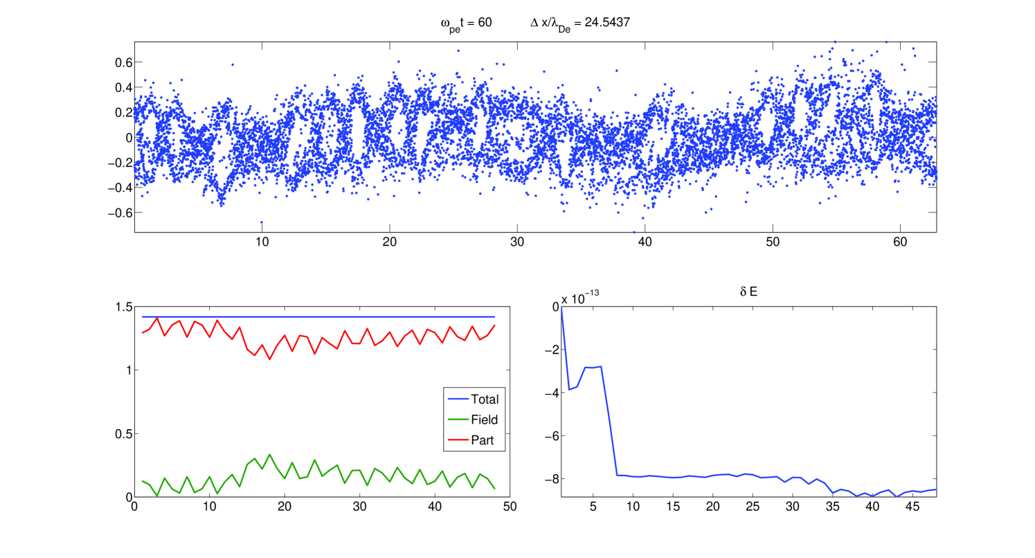
An example of the output obtained from running the unpreconditioned version of the code is given in Fig. 1, where signatures of the two stream instability are clearly visible in the particles phase-space (upper panel), together with the energy evolution and its relative error respect to the initial value (lower panels). This test featured a non-linear iteration tolerance of , particles and cells.
4.1 Test 1 - Different Time Step
From the computational point of view, the time step size may influence the convergence in time dependent problems. Therefore, this section is devoted to analyse the behaviour of the algorithms at different time step. In Fig. 2 we plot the time considered by the code with different . Some interesting considerations can be made.
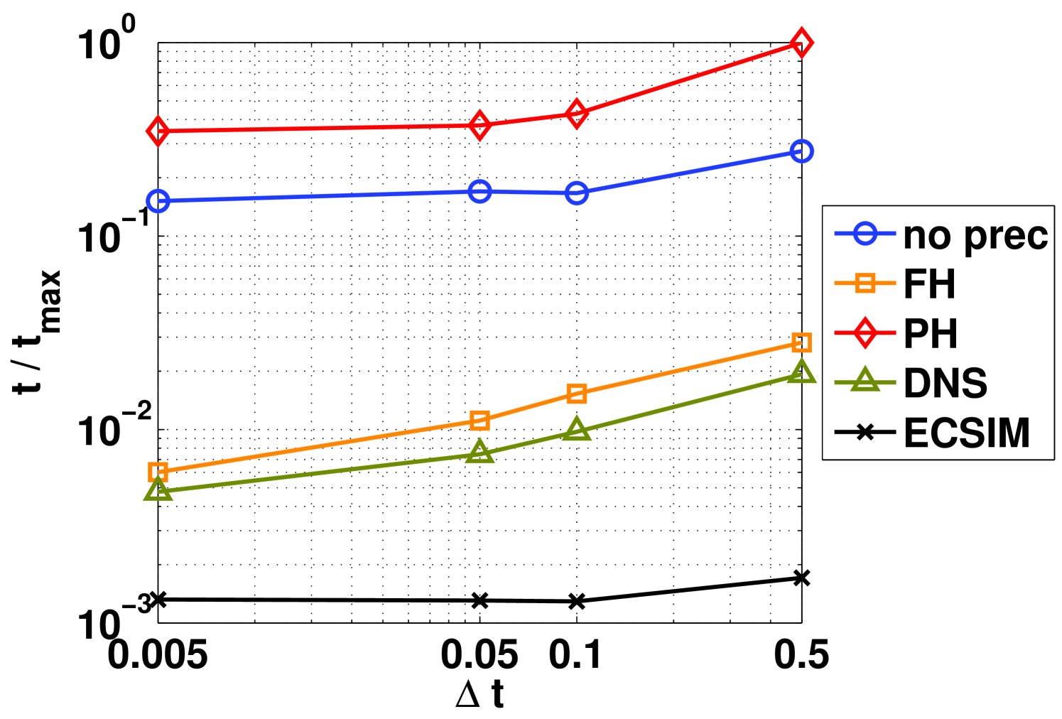
First of all, we notice the ECSIM approach to be the fastest. The ECSIM method requires the computation of a mass matrix, adding extra costs, but it does not use any Newton iteration. Specifically, the cost per cycle in ECSIM is nearly independent of the time step used: this finding is not surprising given the absence of Newton iterations, therefore the cost per cycle is expected to be more constant. However, ECSIM still requires the solution of a linear set of equations, leading to a slight hump in the curve for low . Notice that the cost of ECSIM is nearly the same regardless the solver used, either the MATLAB direct solver or GMRES.
After ECSIM, the following best performing approaches are the DNS and the field hiding (FH). The DNS method is faster by a visible factor, while the performance ratio between the two remains the same as changes. In both the cases the number of Newton iterations increases with and so does the cost per cycle.
Finally, the particle hiding approach and the unpreconditioned ECFIM perform the worst. In fact, the case with the particle hiding is even slower than when no preconditioning is set. Neither of the methods includes a preconditioning capable to capture the field-mediated couplings, leading therefore to a higher number of residual evaluations. In the particular case of the particle hiding, the particle mover does not employ any Eisenstat-Walker inexact convergence [14]. The inexact convergence uses a smart approach to relax the tolerance for the linear GMRES iterations when the non linear Newton convergence is still far from being achieved. This approach limits the cost of the unpreconditioned ECFIM. When the particle hiding is used, the mover moves the particles with a precision requiring the minimum tolerance allowed, leading to a larger overall computational effort.
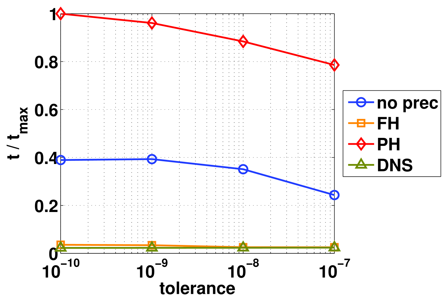
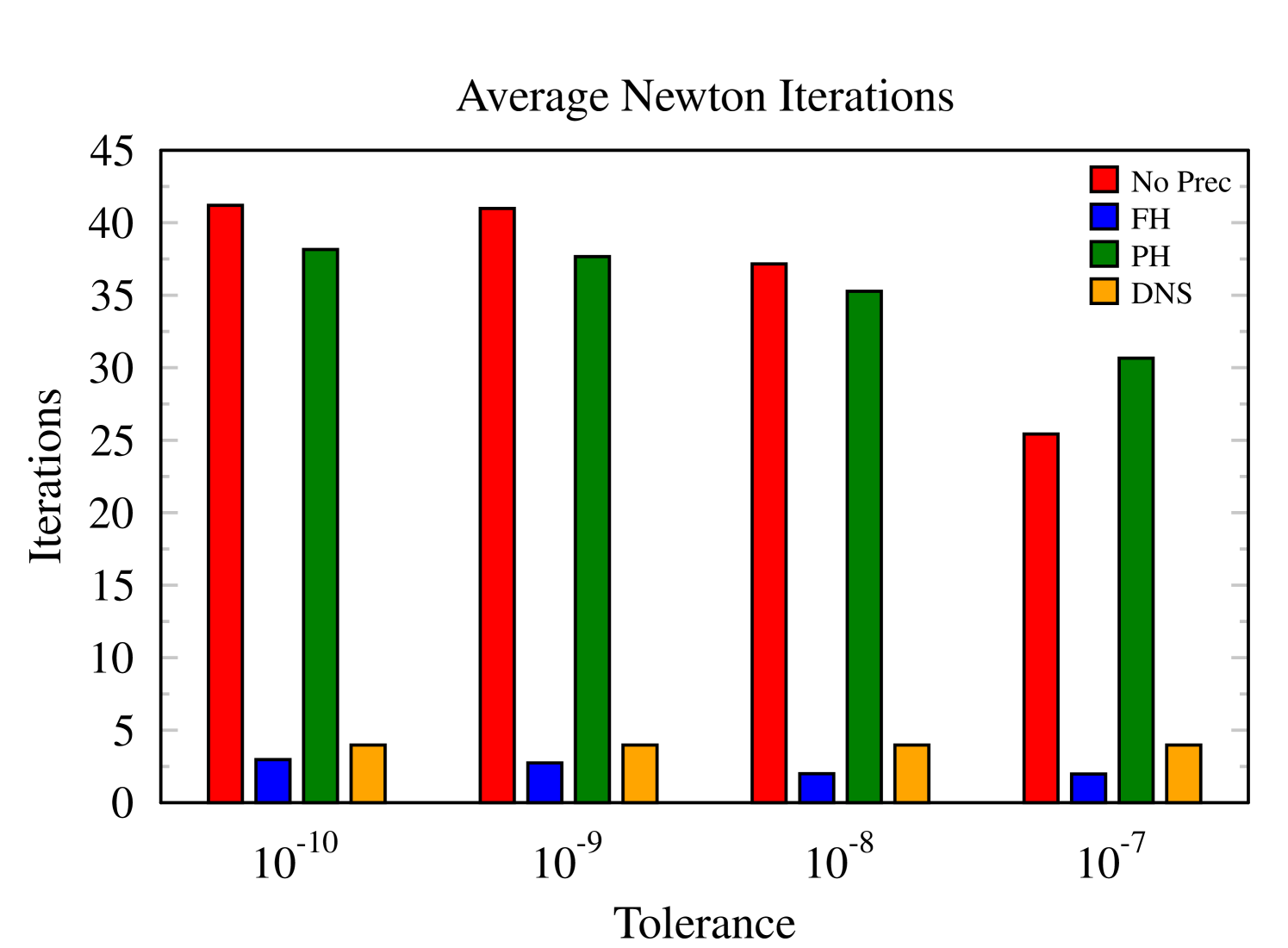
4.2 Test 2 - Different Tolerance of the Newton’s Method
This test shows the influence of different convergence tolerances of the Newton’s iterative method on the simulation performance. The time step is fixed to , and the other parameters are the same as the standard case. The number of iterations of the Newton solver depends on the tolerance considered. Figures 3 and 4 show a certain independence of the chosen tolerance only for the DNS and FH methods, while the other preconditioners reach a saturation point for a tolerance around . In fact we observe an effective improvement in terms of the global performance with these two latter field-hiding preconditioners. In fact, both the field-hiding and DNS drastically reduce the average number of non linear iterations given its capability of capturing better the particle-field couplings with its strategy, leading then to a more rapid Newton convergence. But the field-hiding leads to the smallest number of iterations. This finding is not surprising as the DNS approximates the Jacobian with the Schwarz decomposition, requiring hence more iterations than the case with full a Jacobian evaluation. However, note that each DNS iteration is less computational intensive than that of the field-hiding, which can be explained as with the Jacobian being inverted analytically.
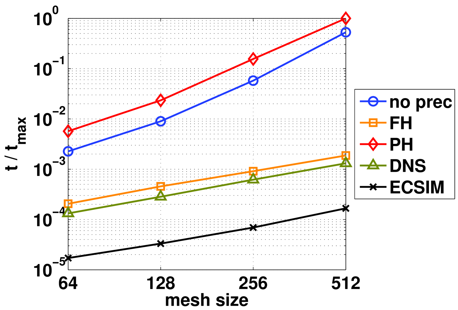
4.3 Test 3 - Different Mesh Size
Of critical interest for practical applications is the performance behaviour when varying the mesh size. Obviously production runs will need large multidimensional grids, so it is important to see how the different implementations scale as the number of cells increases. This test is set such that the mesh size increases as the ratio is kept constant, where and are respectively the number of cells and particles (see Table 1).
| 64 | 128 | 256 | 512 | |
|---|---|---|---|---|
| 10K | 20K | 40K | 80K |
The improvement in the statistic implies an increase in computational effort, which may have a important effect on the couplings in the Maxwell’s equation. Figure 5 reports the relative timing of each method, normalised to the longest run among all tested. As in previous tests, field hiding JFNK and DNS show a better scaling, comparable with that of the ECSIM method. The other two cases (unpreconditioned and particle-hiding) show a less desirable scaling, leading to a faster growth in computational time as the simulation size increases.
To analyse the performance deterioration cause of the unpreconditioned and particle hiding approach, table 2 shows the number of newton iterations for each method at different grid sizes. While the preconditioners field hiding and DNS require only an average of three Newton iterations, the particle hiding and the full coupled algorithm require a fast growing number of iterations. Concretely, the table 2 shows that the non-linear solver may be a bottleneck if it is not carefully preconditioned. Furthermore, the raise in Newton iteration is a clear evidence of the the different asymptotic behaviour in figure 5.
| Mesh size | No prec | FH | PH | DNS |
|---|---|---|---|---|
| 64 | 41.33 | 2.96 | 38.315 | 3.98 |
| 128 | 70.41 | 2.98 | 69.71 | 3.99 |
| 256 | 204.10 | 2.99 | 210.20 | 4.0 |
| 512 | 843.27 | 2.99 | 612.64 | 4.0 |
The lesson of this test is that the couplings across the domain carried by the fields need to be preconditioned away from the non linear iteration or the costs of the simulation balloon as the simulation size increases.
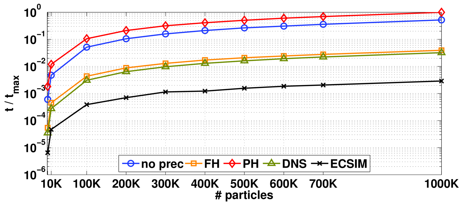
4.4 Test 4 - Different Number of Particles
The final test proposed here regards the influence of the number of particles on the simulation performance, when the grid is not also increased. The interest of this test is that as the number of particles is increased the noise of the PIC simulation decreases. We can then test the effect of noise on convergence.
Unlike the previous plots, results in Fig. 6 are shown in a semi-logarithmic scale for a better readability. We chose a broad range of cases, spanning from that with a very few particles simulated (i.e. ) through the case with a great number of particles in the system (i.e. ). As could be expected, the reduction in noise at higher number of particles leads to a saturation of the computational cost. This feature seems to be of particular importance given the kinetic nature of these methods, allowing for the usage of a large number of particles without dramatically increasing the computational time. The best performance is again achieved by ECSIM. Also, the two methods sharing the field-hiding method show a very similar behaviour featuring nearly the same execution time. This was somehow expected given their common original approach, even though the DNS method seems to be not particularly more affective than the original field-hiding preconditioner. This is in line with the the concept of DNS being conceived for a memory use improvement rather than execution time.
5 Conclusions
In this paper we presented a set of different strategies to improve the computing performance of fully implicit Particle-in-Cell (PIC) codes. Unlike semi-implicit PICs, which make use of a linear approximation to improve performance, we consider here no approximations of the original formulation and focus only on advanced non-linear solvers that still produce the same exact result. Due to the heavy CPU and memory consumption requested by the iteration of the entire non-linear system, the fully implicit approach has long been considered expendable over the semi-implicit counterpart. This concern, however, is largely eliminated when preconditioners are used. In this work we proved that the computation with fully implicit PICs can be significantly improved whether a careful application of ad-hoc preconditioning methods be applied. The semi-implicit method remains the fastest, but the fully implicit methods come now close second.
The first preconditioner method considered here is found in previous literature [27] and named particle-hiding after its approach of segregating the particle mover from the field solver in the non-linear JFNK iteration. Particles are still continuously updated within the iterative cycle using the fields information, but now the particles velocity is no longer considered as part of the residual convergence, consequently leading to a lower number of iterations and a strong reduction of the memory demanded due to the non storage of the particles information. The downside is that for each residual evaluation, all particles still need to be moved, so that this approach still relies on the full mutual coupling between particles and fields, which conducts to further computational costs.
We have then proposed a further improvement based upon the fact that are actually the fields being the coupling source in the system rather than the particles. Particles do not directly interact with each other, their interaction is provided by the field. Mathematically, the fields are coupled with each particles while the particles just need the updated field information to compute their new position and velocity. The approach is based on a complementary variant of the previous method, and is named field-hiding after its application to the field information instead of particles’. It is now the field solver to be segregated out of the residual computation, so that the iteration is only performed over the particles velocity. Having removed all direct couplings from the JFNK calculation and having relegated all field couplings to the preconditioner, this approach is shown to perform faster then the previous one. However, the memory consumption downside is yet present, as the method requires a memory allocation as large as the number of particles considered in the system, which may become very heavy for real-system simulations.
In order to further relax this issue, a different preconditioner based on the field-hiding approach has been presented. Given the independence of the particles from each other, the Jacobian matrix appears to have all the cross-over derivatives equal to zero. We can then consider to eliminate the use of the Krylov space and resolve the linear part of the Newton iteration using a Schwarz decomposition. The JFNK is then no longer needed, each particles is solved independently via a direct newton iteration based on the Schwarz decomposed Jacobian computed and inverted analytically particle by particle. In doing so, we combine the two main advantages of the two previous preconditioners: 1) not having to deal with a large dimensional array and 2) not dealing with the main couplings directly inside the non-linear iterative loop.
This latter approach is shown to lead to a lower number of iterations required in the non-linear solver and to the fastest CPU performance. From the tests presented, we can in fact confirm that the Direct-Newton-Schwarz (DNS) method is the fastest to converge. The DNS also eliminates the need to reserve memory for the particle iterative solution as each particle is solved independently and directly. DNS comes second only to the semi-implicit ECSIM method, which yet relies on a completely different approximation approach.
In conclusion, we observe how the field-hiding preconditioner approach is reported here as the most promising, especially when coupled with a DNS formulation, avoiding Krylov subspace solvers altogether. In fact, all the tests with different number of particles, different mesh, different Newton iteration tolerance and different time step have shown that the field-hiding approach, and especially its DNS implementation, is the best fully non-linear system. While the ECsim semi-implicit approach is still the fastest, we note that its extension to relativistic system does not appear to be straight-forward, while that of the DNS fully implicit method is.
Appendix A MATLAB Listing of the unpreconditioned residual
We refer the reader to [20] for any unclear aspect of the program. Especially the implementation of the interpolation function using MATLAB matrices is not trivial, and all details are fully explained in the reference.
Appendix B MATLAB Listing of the residual with particle hiding
Appendix C MATLAB Listing of the residual with field hiding
Acknowledgments
This work is funded by the USAF EOARD Grant No.FA2386-14-1-5002. EC acknowledges support from the Leverhulme Research Project Grant Ref. 2014-112 and would like to thank Dr. Cesare Tronci for the enlighting discussions.
References
- [1] C.K. Birdsall and A.B. Langdon. Plasma Physics Via Computer Simulation. Taylor & Francis, London, 2004.
- [2] K. J. Bowers, B. J. Albright, L. Yin, W. Daughton, V. Roytershteyn, B. Bergen, and T. J. T. Kwan. Advances in petascale kinetic plasma simulation with VPIC and Roadrunner. Journal of Physics Conference Series, 180(1):012055–+, July 2009.
- [3] J. U. Brackbill and B. I. Cohen, editors. Multiple time scales., 1985.
- [4] J.U. Brackbill and D.W. Forslund. An implicit method for electromagnetic plasma simulation in two dimension. J. Comput. Phys., 46:271, 1982.
- [5] Xiao-Chuan Cai, William D Gropp, David E Keyes, Robin G Melvin, and David P Young. Parallel newton–krylov–schwarz algorithms for the transonic full potential equation. SIAM Journal on Scientific Computing, 19(1):246–265, 1998.
- [6] J Candy and RE Waltz. Anomalous transport scaling in the diii-d tokamak matched by supercomputer simulation. Physical review letters, 91(4):045001, 2003.
- [7] Emanuele Cazzola, Davide Curreli, Stefano Markidis, and Giovanni Lapenta. On the ions acceleration via collisionless magnetic reconnection in laboratory plasmas. Physics of Plasmas, 23(11):112108, 2016.
- [8] Sydney Chapman and Thomas George Cowling. The mathematical theory of non-uniform gases: an account of the kinetic theory of viscosity, thermal conduction and diffusion in gases. Cambridge university press, 1970.
- [9] Guangye Chen and Luis Chacon. A multi-dimensional, energy-and charge-conserving, nonlinearly implicit, electromagnetic vlasov–darwin particle-in-cell algorithm. Computer Physics Communications, 197:73–87, 2015.
- [10] Guangye Chen, Luis Chacón, and Daniel C Barnes. An energy-and charge-conserving, implicit, electrostatic particle-in-cell algorithm. J. Comput. Phys., 230(18):7018–7036, 2011.
- [11] Guangye Chen, Luis Chacón, and Daniel C Barnes. An efficient mixed-precision, hybrid cpu–gpu implementation of a nonlinearly implicit one-dimensional particle-in-cell algorithm. J. Comput. Phys., 231(16):5374–5388, 2012.
- [12] Guangye Chen, Luis Chacón, Christopher A Leibs, Dana A Knoll, and William Taitano. Fluid preconditioning for newton–krylov-based, fully implicit, electrostatic particle-in-cell simulations. J. Comput. Phys., 258:555–567, 2014.
- [13] R.W. Hockney and J.W. Eastwood. Computer simulation using particles. Taylor & Francis, 1988.
- [14] C. T. Kelley. Iterative methods for linear and nonlinear equations. SIAM, Philadelphia, 1995.
- [15] H. Kim, L. Chacòn, and G. Lapenta. Fully implicit particle-in-cell algorithm. Bull. Am. Phys. Soc., 50:2913, 2005.
- [16] Dana A Knoll and David E Keyes. Jacobian-free newton–krylov methods: a survey of approaches and applications. J. Comput. Phys., 193(2):357–397, 2004.
- [17] A.B. Langdon, BI Cohen, and A Friedman. Direct implicit large time-step particle simulation of plasmas. J. Comput. Phys., 51:107–138, 1983.
- [18] G. Lapenta, J .U. Brackbill, and P. Ricci. Kinetic approach to microscopic-macroscopic coupling in space and laboratory plasmas. Phys. Plasmas, 13:055904, 2006.
- [19] Giovanni Lapenta. Particle simulations of space weather. J. Comput. Phys., 231(3):795–821, 2012.
- [20] Giovanni Lapenta. Particle-based simulation of plasmas. In Plasma Modeling, 2053-2563, pages 4–1 to 4–37. IOP Publishing, 2016.
- [21] Giovanni Lapenta. Exactly energy conserving semi-implicit particle in cell formulation. Journal of Computational Physics, 334:349 – 366, 2017.
- [22] Giovanni Lapenta, Diego Gonzalez-Herrero, and Elisabetta Boella. Multiple-scale kinetic simulations with the energy conserving semi-implicit particle in cell method. Journal of Plasma Physics, 83(2), 2017.
- [23] Giovanni Lapenta and Stefano Markidis. Particle acceleration and energy conservation in particle in cell simulations. Physics of Plasmas (1994-present), 18(7):072101, 2011.
- [24] Damian Alvarez Mallon, Norbert Eicker, Maria Elena Innocenti, Giovanni Lapenta, Thomas Lippert, and Estela Suarez. On the scalability of the clusters-booster concept: a critical assessment of the deep architecture. In Proceedings of the Future HPC Systems: the Challenges of Power-Constrained Performance, page 3. ACM, 2012.
- [25] S. Markidis, E. Camporeale, D. Burgess, Rizwan-Uddin, and G. Lapenta. Parsek2D: An Implicit Parallel Particle-in-Cell Code. In N. V. Pogorelov, E. Audit, P. Colella, & G. P. Zank, editor, Astronomical Society of the Pacific Conference Series, volume 406 of Astronomical Society of the Pacific Conference Series, pages 237–+, April 2009.
- [26] S. Markidis, G. Lapenta, and Rizwan-uddin. Multi-scale simulations of plasma with iPIC3D. Mathematics and Computers and Simulation, 80:1509–1519, 2010.
- [27] Stefano Markidis and Giovanni Lapenta. The energy conserving particle-in-cell method. J. Comput. Phys., 230(18):7037–7052, 2011.
- [28] Youcef Saad and Martin H Schultz. Gmres: A generalized minimal residual algorithm for solving nonsymmetric linear systems. SIAM Journal on scientific and statistical computing, 7(3):856–869, 1986.
- [29] Luís O Silva, Michael Marti, Jonathan R Davies, Ricardo A Fonseca, Chuang Ren, Frank S Tsung, and Warren B Mori. Proton shock acceleration in laser-plasma interactions. Physical Review Letters, 92(1):015002, 2004.
- [30] Lorenzo Sironi, Anatoly Spitkovsky, and Jonathan Arons. The maximum energy of accelerated particles in relativistic collisionless shocks. The Astrophysical Journal, 771(1):54, 2013.
- [31] A. Taflove and Susan C. Hagness. Computational Electrodynamics: The Finite-Difference Time-Domain Method. Artech House Publishers, Norwood, 2005.
- [32] William T Taitano, Dana A Knoll, Luis Chacón, and Guangye Chen. Development of a consistent and stable fully implicit moment method for vlasov–ampère particle in cell (pic) system. SIAM Journal on Scientific Computing, 35(5):S126–S149, 2013.
- [33] H. X. Vu and J. U. Brackbill. Celest1d: An implicit, fully-kinetic model for low-frequency, electromagnetic plasma simulation. Comput. Phys. Comm., 69:253, 1992.