Compiler Optimization: A Case for the Transformation Tool Contest

Sebastian Buchwald Edgar Jakumeit Karlsruhe Institute of Technology (KIT) buchwald@kit.edu

(March 26, 2011)

1 Introduction

An optimizing compiler consists of a front end parsing a textual programming language into an intermediate representation (IR), a middle end performing optimizations on the IR, and a back end lowering the IR to a target representation (TR) built of operations supported by the target hardware. In modern compiler construction graph-based IRs are employed. Optimization and lowering tasks can then be implemented with graph transformation rules.

The participating tools are required to solve the following challenges:

Local optimizations: replace an IR pattern of limited size and only local graph context by another semantically equivalent IR pattern which is cheaper to execute or which enables further optimizations. For instance, given the associativity of the ’+’-operator, the transformation $(x+1)+2\Rightarrow x+(1+2)\Rightarrow x+3$ can be performed by local optimizations.
Instruction selection: transforms the intermediate representation into the target representation. While both representations are similar in structure, the TR operations are often equivalent to a small pattern of IR operations, i.e. one TR operation covers an IR pattern (it may be equivalent to several different IR patterns). Thus instruction selection can be approached by applying rules rewriting IR patterns to TR nodes, until the whole IR graph was covered and transformed to a least cost TR graph.

The primary purpose of these challenges is to evaluate the participating tools regarding performance. The ability to apply rules in parallel should be beneficial for the instruction selection task due to the locality of the rules and a high degree of independence in between the rules. It could be advantageous for the optimization task, too, but intelligent traversal strategies might have a higher impact there. Secondary aims are fostering tool interoperability regarding the GXL standard format and testing the ability to visualize medium sized real world graphs.

We provide the following resources on the case website [2]:

•

This case description.
•

Input graphs of various sizes in GXL format.
•

The needed meta models are contained in the GXL files.

2 A Graph-Based Intermediate Representation

The intermediate representation to be used is a simplified version of the graph-based intermediate representation Firm ¹¹1www.libfirm.org. Within Firm, nodes represent basic operations, e.g. loading a value from an address or adding two values. Edges indicate dependencies between nodes, e.g. an Add depends on its two operands. Each operation is located within a Block²²2also known as basic block. For the represented program all nodes within the same Block are executed together, i.e. if one node within a Block is executed then all nodes within the Block must be executed.

Refer to caption — Figure 1: Program graph of a minimum plus one function, with block containment visualized as containment left, and the plain graph right.

Figure 1 shows the program graph of our reference solution [4] for the following C-function:

⬇

int MinPlus(int x, int y)

{

int min;

if (x < y) {

min = x;

}

else {

min = y;

}

return min + 1;

}

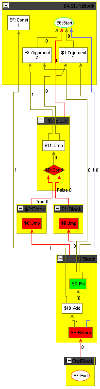
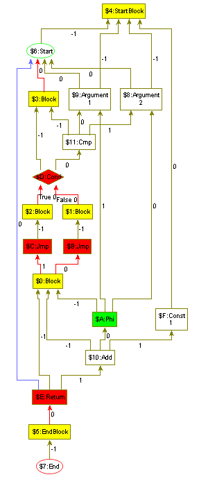
The program execution starts at Start, which also produces the initial memory state and the given Arguments. Start and the Arguments belong to the special StartBlock. The Cmp compares the arguments and Cond represents a conditional jump depending on the result of the comparison. After executing the Jmp of the then- or else-Block the program execution continues at Block $0. The Phi originates form the static single assignment form [5] which is required for a concise graph-based IR. It chooses one of its operands depending on the previously executed block. For instance, the Phi selects Argument $2$ if the Cond was evaluated to False and Argument $1$ if the Cond was evaluated to True. The Return returns the value selected by the Phi. The end of the program execution is represented by the special EndBlock which by convention contains exactly one End.

Each node has ordered outgoing edges, which is indicated by the position attribute of the edges. Edges representing the containment to a Block have position $-1$ ; the operands start at position $0$ . There are several edge types:

Dataflow: Models the flow of data from an operation to another one.
Memory: Memory edges are used to ensure an order for memory operations.
Controlflow: Models possible execution paths through the program.
True: Control flow if a condition jump is evaluated to true.
False: Control flow if a condition jump is evaluated to false.
Keep: Needed to model infinite loops, see description of End.

The direction of the edges is reversed to the direction of the flow (it follows the dependencies). For instance, start has only incoming edges.

The following list describes all node types (the ^∗ marks the types which are of relevance for the instruction selection task):

Block

A basic block. All outgoing edges point to possible execution predecessors. The incoming Dataflow edges define the contained operations. In the figures the contained operations are shown as containment in the Block node for easier readability, the right subfigure of Figure 1 displays the plain graph structure underneath.

StartBlock

The start block.

Start

The starting point of the program. Produces initial control flow and memory state.

Argument

The arguments of the program. The position attribute indicates which argument is represented.

EndBlock

The end block.

End

Nodes which are not reachable by the End can be removed from the graph. Since infinite loops may never reach the EndBlock, Keep edges are inserted to prevent the removal of such a loop.

Phi

A Phi selects the operand of the previously executed Block from the operands available. This implies that the number of operands of a Phi node must be equivalent to the number of control flow predecessors of the Block it is contained in. Furthermore the position attributes of the operand edges of the Phi node must be equal to the position attributes of the corresponding control flow edges of the containing Block node.

Jmp^∗

A jump to a Block.

Cond^∗

A conditional jump. The operand must be a Cmp or another node producing a value $\in\{0,1\}$ , e.g. a Const.

Return

Returns a value. The first operand must be the current memory state and the second operand the return value.

Const^∗

A constant value. The value of the constant of integer type is presented by the value attribute. A Const is always located in the StartBlock.

SymConst^∗

A symbolic constant. A SymConst is used to represent the address of some global data, e.g. arrays. The symbol attribute of string type represents the name of the global data. A SymConst is always located in the StartBlock.

Load^∗

Load a value from a given address. The first operand is the current memory state and the second operand is the address. The Load produces a new memory state. The volatile attribute indicates whether the value at the corresponding memory address can be changed by some other thread. For instance, two consecutive volatile Loads from the same address cannot be merged.

Store^∗

Stores a value to a given address. The first operand is the current memory state, the second operand is the address and the third operand the value that should be stored. Similar to the Load, a Store also has a volatile attribute.

Sync

Synchronize multiple memory operations. The Sync is used to represent that some memory operations are not in any particular order. For instance, Loads of different array elements $a[i]$ , $a[i+1]$ may not be ordered.

Not^∗

Bitwise complement.

Binary^∗

An operation with two operands. Each binary operation has two boolean attributes: associative and commutative. The following binary operations are supported:

•

Add^∗
•

Sub^∗
•

Mul^∗
•

Div^∗
•

Mod^∗
•

Shl^∗—shift left, fill up with zero
•

Shr^∗—shift right, fill up with zero
•

Shrs^∗—shift right signed, fill up with sign bit ( $1$ if negative, $0$ otherwise)
•

(bitwise) And^∗
•

(bitwise) Or^∗
•

(bitwise) Eor^∗—exclusive or
•

Cmp^∗—compare two values.
The relation attribute indicates the checked relation, i.e. one of FALSE, GREATER, EQUAL, GREATER_EQUAL, LESS, NOT_EQUAL, LESS_EQUAL, and TRUE.

3 Getting started: Verifier

To get started you can create some rules that check your graph for validity. This may include the following checks:

•

There is only one Start.
•

There is only one End.
•

A Dataflow edge to a Block always has position $-1$ .
•

Constants are only located in the StartBlock.
•

A Phi has as many operand Dataflow edges as the Block it is located in Controlflow predecessors.
•

The operand Dataflow edges of a Phi are linked to the Controlflow edges of the Block it is contained in via the position attribute in those edges - are they ascending from 0 on without gaps?

The verifier is not part of the challenge, but it might be helpful in checking the correctness of your solution of the following tasks.

4 Task 1: Local Optimizations

The first task is to optimize programs using local optimizations, i.e. rules with a pattern of fixed size and only local graph context.

4.1 Constant Folding

Constant folding means to evaluate an operation with only constants operands, e.g. to transform $1+2$ into $3$ . Constant folding of data flow operations is a straight-forward task, a good deal more complicated is constant folding including control flow, replacing conditional jumps with constant operands by unconditional jumps.

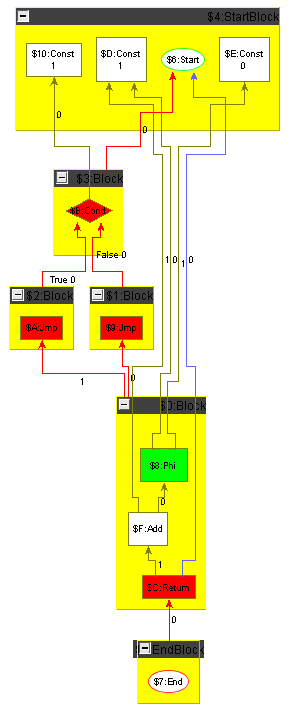
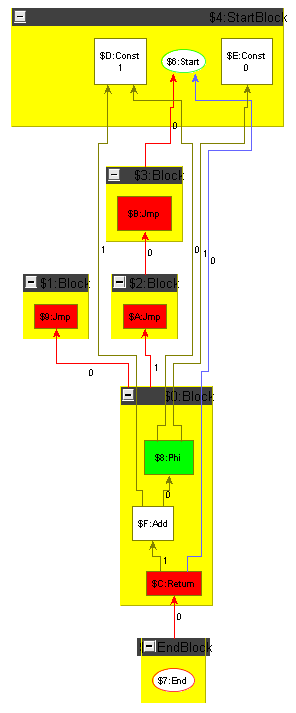
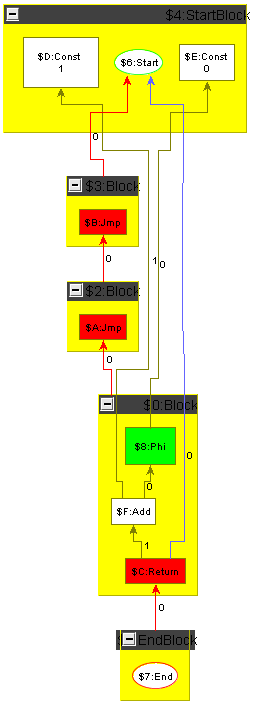
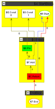
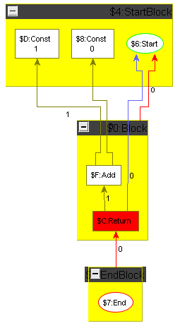
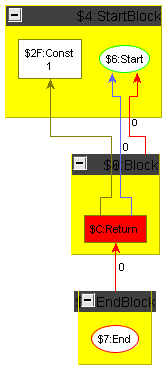
To ease the challenge for participants not knowledgeable in compiler construction we show how to carry out constant folding including control flow on an example graph. The example graph is the minimum plus one graph introduced in the previous section, but with the arguments replaced by constants; it is shown in the following section, Figure 5, left side. Folding starts with the Cmp node comparing two constant values: it is folded to a constant giving the result of the comparison, which is $1$ denoting $true$ in our case; the result is displayed in Figure 2a. Then the Cond node depending only on the constant created in the previous step is folded, i.e. replaced by an unconditional Jmp; the result is shown in Figure 2b. In the next step, we remove the unreachable false Block. When a block is removed, the Phis in the blocks succeeding it must get adapted, i.e. the operands which resulted from executing that block must get removed. Additionally the position attributes of the control flow edges and of the data flow edges of the Phi operands must be decremented from the correct position on. The result is shown in Figure 3a. Now the empty blocks denoting a useless jump cascade can get removed and the Phi folded; a Phi with only one dependency edge is superfluous as there is no decision to be taken at runtime any more, it can get replaced by relinking its users directly to its input value. Removing the empty blocks first and folding the Phi afterwards (we could reverse this or do it in parallel), we reach via Figure 3b the situation given in Figure 4a. Folding the Add node now only depending on two constants, we reach the end result of the optimization, a function returning the constant value $1$ .

To make the tools comparable, there will be a test suite of multiple programs (in GXL format) that can be optimized by local optimizations.

4.2 Extension

You may challenge the other participants by adding your own test programs to the tests suite. The only requirement is that the corresponding optimization is a local optimization. This offers the opportunity to highlight strong points of your tool.

5 Task 2: Instruction Selection

The second task is to perform instruction selection, i.e. to transform the intermediate representation into a target-specific representation. We assume a very simple target architecture resulting in a TR which is structurally nearly identical to the IR, with the sole exception of “immediates” which may be encoded directly in the target instructions³³3More precisely, we assume some kind of simple RISC machine; the more interesting case of a CISC machine, where target operations can contain a memory access, giving rise to non-trivial IR patterns to be covered, is too complicated for this contest.

All operations that must be transformed by instruction selection are marked with a ’^∗’. For each operation Op there is a target-specific operation TargetOp representing an operation on registers, e.g. R1 = add R2, R3. For each binary operation Op there is an additional target-specific operation TargetOpI, which has one constant operand, e.g. R1 = add R2, 42. It represents an IR pattern Op(x, Const). The value of the constant is called “immediate” and is stored in the additional value attribute. For non-commutative binary operations the Const must be at the outgoing edge with position $1$ . For Load and Store there are in addition target-specific operations LoadI and StoreI with an additional attribute symbol which holds a symbolic constant; they represent IR patterns Load(mem, SymConst) and Store(mem, SymConst, x).

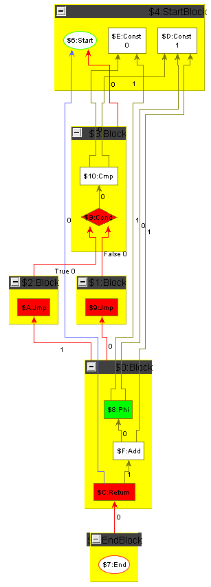
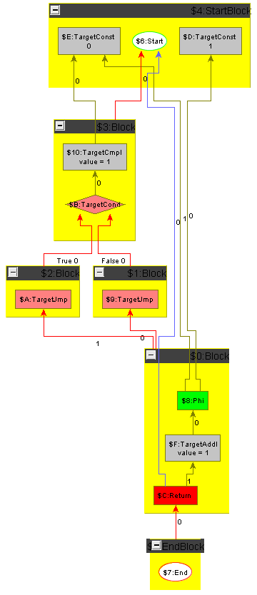
The goal of this task is to perform optimal instruction selection with respect to the number of resulting operations. This means an operation with immediate is always better than the same operation without immediate. Figure 5 shows the minimum plus one function on constant values not optimized away by constant folding, before and after instruction selection. Performance hint: the setup given allows to process all operations with immediate and then all operations without immediate in parallel.

6 Evaluation criteria

For each task tackled the authors should give a short overview of their solution. Furthermore, the solution should contain some statements regarding the following criteria:

Completeness: Which programs of the test suite are covered by the solution.
Performance: How long does your solution need to optimize/transform the programs. How much memory does your solution need?
Conciseness: How many rules/lines/words/graphical elements do you need?
Purity: Is your solution entirely made of graph transformations? Do you need imperative/functional/logical glue code? What is the relationship between the graph transformation and the conventional programming part?

References

[1]
[2] Available at www.grgen.net/ttc2011_compiler_case/.
[3] Available at www.libfirm.org.
[4] Sebastian Buchwald & Edgar Jakumeit (2011): Solving the TTC 2011 Compiler Optimization Case with GrGen.NET. In Van Gorp et al. [6].
[5] B. K. Rosen, M. N. Wegman & F. K. Zadeck (1988): Global value numbers and redundant computations. In: Proceedings of the 15th ACM SIGPLAN-SIGACT symposium on Principles of programming languages, POPL ’88, ACM, New York, NY, USA, pp. 12–27, 10.1145/73560.73562.
[6] Pieter Van Gorp, Steffen Mazanek & Louis Rose, editors (2011): TTC 2011: Fifth Transformation Tool Contest, Zürich, Switzerland, June 29-30 2011, Post-Proceedings. EPTCS.