Complexity of and Algorithms for Borda Manipulation
Abstract
We prove that it is NP-hard for a coalition of two manipulators to compute how to manipulate the Borda voting rule. This resolves one of the last open problems in the computational complexity of manipulating common voting rules. Because of this NP-hardness, we treat computing a manipulation as an approximation problem where we try to minimize the number of manipulators. Based on ideas from bin packing and multiprocessor scheduling, we propose two new approximation methods to compute manipulations of the Borda rule. Experiments show that these methods significantly outperform the previous best known approximation method. We are able to find optimal manipulations in almost all the randomly generated elections tested. Our results suggest that, whilst computing a manipulation of the Borda rule by a coalition is NP-hard, computational complexity may provide only a weak barrier against manipulation in practice.
Introduction
Voting is a simple mechanism to combine preferences in multi-agent systems. Unfortunately, results like those of Gibbrard-Sattertwhaite prove that most voting rules are manipulable. That is, it may pay for agents to mis-report their preferences. One appealing escape from manipulation is computational complexity (?). Whilst a manipulation may exist, perhaps it is computationally too difficult to find? Unfortunately, few voting rules in common use are NP-hard to manipulate with the addition of weights to votes. The small set of voting rules that are NP-hard to manipulate with unweighted votes includes single transferable voting, 2nd order Copeland, ranked pairs (all with a single manipulator), and maximin (with two manipulators) (?; ?; ?).
Borda is probably the only commonly used voting rule where the computational complexity of unweighted manipulation remains open. ? (?) observe that:
“The exact complexity of the problem [manipulation by a coalition with unweighted votes] is now known with respect to almost all of the prominent voting rules, with the glaring exception of Borda”
It is known that computing a manipulation of Borda is NP-hard when votes are weighted (?), and polynomial when votes are unweighted and there is just a single manipulator (?). With a coalition of manipulators and unweighted votes, it has been conjectured that the problem is NP-hard (?).
One of our most important contributions is to close this question. We prove that computing a manipulation of Borda with just two manipulators is NP-hard. As a consequence, we treat computing a manipulation as an approximation problem in which we try to minimize the number of manipulators required. We propose two new approximation methods. These methods are based on intuitions from bin packing and multiprocessor scheduling. Experiments show that these methods significantly outperform the previous best known approximation method. They find optimal manipulations in the vast majority of the randomly generated elections tested.
Background
The Borda rule is a scoring rule proposed by Jean-Charles de Borda in 1770. Each voter ranks the candidates. A candidate receives a score of for appearing in place. The candidate with the highest aggregated score wins the election. As is common in the literature, we will break ties in favour of the coalition of the manipulators. The Borda rule is used in parliamentary elections in Slovenia and, in modified form, in elections within the Pacific Island states of Kiribati and Nauru. The Borda rule or modifications of it are also used by many organizations and competitions including the Robocup autonomous robot soccer competition, the X.Org Foundation, the Eurovision song contest, anf in the election of the Most Valuable Player in major league baseball. The Borda rule has many good features. For instance, it never elects the Condorcet loser (a candidate that loses to all others in a majority of head to head elections). However, it may not elect the Condorcet winner (a candidate that beats all others in a majority of head to head elections).
We will number candidates from 1 to . We suppose a coalition of agents are collectively trying to manipulate a Borda election to ensure a preferred candidate wins. We let be the score candidate receives from the votes cast so far. A score vector gives the scores of the candidates from a set of votes. Given a set of votes, we define the gap of candidate as . For to win, we need additional votes that add a score to candidate which is less than or equal to . Note that if is negative for any , then cannot win and manipulation is impossible.
Our NP-hardness proof uses a reduction from a specialized permutation problem that is strongly NP-complete (?).
Definition 1 (Permutation Sum)
Given integers where , do there exist two permutations and of 1 to such that ?
One of our main contributions is to prove that computing a manipulation of the Borda rule is NP-hard, settling an open problem in computational social choice.
Complexity of manipulation
The unweighted coalition manipulation problem (UCM) is to decide if there exist votes for a coalition of unweighted manipulators so that a given candidate wins. As in (?), we suppose that the manipulators have complete knowledge about the scores given to the candidates from the votes of the non-manipulators.
Theorem 1
Unweighted coalition manipulation for the Borda rule is NP-complete with two manipulators.
Proof: Clearly the problem is in NP. A polynomial witness is simply the votes that the manipulators cast which make the chosen candidate win.
To show NP-hardness, we reduce a Permutation Sum problem over integers, to , to a manipulation problem with candidates. By Lemma 1, we can construct an election in which the non-manipulators cast votes to give the score vector:
where is a constant and . We claim that two manipulators can make candidate win such an election iff the Permutation Sum problem has a solution.
() Suppose we have two permutations and of to with . We construct two manipulating votes which have the scores:
Since , these give a total score vector:
As and we tie-break in favour of the manipulators, candidate wins.
() Suppose we have a successful manipulation. To ensure candidate beats candidate , both manipulators must put candidate in first place. Similarly, both manipulators must put candidate in last place otherwise candidate will will beat our preferred candidate. Hence the final score of candidate is . The gap between the final score of candidate and the current score of candidate (where ) is . The sum of these gaps is . If any candidate to gets a score of then candidate will be beaten. Hence, the two scores of have to go to the least dangerous candidate which is candidate .
The votes of the manipulators are thus of the form:
Where and are two permutations of to . To ensure candidate beats candidate for , we must have:
Rearranging this gives:
Since and , there can be no slack in any of these inequalities. Hence,
That is, we have a solution of the Permutation Sum problem.
Recall that we have assumed that the manipulators have complete knowledge about the scores from the votes of the non-manipulators. The argument often put forward for such an assumption is that partial or probabilistic information about the votes of the non-manipulators will add to the computational complexity of computing a manipulation.
Approximation methods
NP-hardness only bounds the worst-case complexity of computing a manipulation. Given enough manipulators, we can easily make any candidate win. We consider next minimizing the number of manipulators required. For example, Reverse is a simple approximation method proposed to compute Borda manipulations (?). The method constructs the vote of each manipulator in turn: candidate is put in first place, and the remaining candidates are put in reverse order of their current Borda scores. The method continues constructing manipulating votes until wins. A long and intricate argument shows that Reverse constructs a manipulation which uses at most one more manipulator than is optimal.
Example 1
Suppose we have 4 candidates, and the 2 non-manipulators have cast votes: and . Then we have the score vector . We use Reverse to construct a manipulation that makes candidate win. Reverse first constructs the vote: . The score vector is now . Reverse next constructs the vote: . (It will not matter how ties between , and are broken). The score vector is now . Finally, Reverse constructs the vote: . The score vector is . Hence, Reverse requires 3 manipulating votes to make candidate win. As we see later, this is one more vote than the optimal.
Manipulation matrices
We can view Reverse as greedily constructing a manipulation matrix. A manipulation matrix is an by matrix, where iff the th manipulator adds a score of to candidate . A manipulation matrix has the properties that each of the rows is a permutation of 0 to , and the sum of the th column is less than or equal to , the maximum score candidate can receive without defeating . Reverse constructs this matrix row by row.
Our two new approximation methods break out of the straightjacket of constructing a manipulation matrix in row wise order. They take advantage of an interesting result that relaxes the constraint that each row is a permutation of 0 to . This lets us construct a relaxed manipulation matrix. This is an by matrix that contains copies of 0 to in which the sum of the th column is again less than or equal to . In a relaxed manipulation matrix, a row can repeat a number provided other rows compensate by not having the number at all.
Theorem 2
Suppose there is an by relaxed manipulation matrix . Then there is by manipulation matrix with the same column sums.
Proof: By induction on . In the base case, and we just set for . In the inductive step, we assume the theorem holds for all relaxed manipulation matrices with rows. Let be the sum of the th column of . We use a perfect matching in a suitable bipartite graph to construct the first row of and then appeal to the induction hypothesis on an by relaxed manipulation matrix constructed by removing the values in the first row from .
We build a bipartite graph between the vertices and for and . represent the scores assigned to the first row of , whilst represent the columns of from where these will be taken. We add the edge to this bipartite graph for each , and where . Note that there can be multiple edges between any pair of vertices. By construction, the degree of each vertex is .
Suppose we take any . By a simple counting argument, the neighborhood of must be at least as large as . Hence, the Hall condition holds and a perfect matching exists (?). Consider an edge in such a perfect matching. We construct the first row of by setting . As this is a matching, each occurs once, and each column is used exactly one time. We now construct an by matrix from by removing one element equal to from each column . By construction, each value occurs times, and the column sums are now . Hence it is a relaxed manipulation matrix. We can therefore appeal to the induction hypothesis. This gives us an by manipulation matrix with the same column sums as .
We can extract from this proof a polynomial time method to convert a relaxed manipulation matrix into a manipulation matrix. Hence, it is enough to propose new approximation methods that construct relaxed manipulation matrices. This is advantageous for greedy methods like those proposed here as we have more flexibility in placing later entries into good positions in the manipulation matrix.
Largest Fit
Our first approximation method, Largest Fit is inspired by bin packing and multiprocessor scheduling. Constructing an by relaxed manipulation matrix is similar to packing objects into bins with a constraint on the capacity of the different bins. In fact, the problem is even similar to scheduling unit length jobs on different processors with a constraint on the total memory footprint of the different jobs running at every clock tick. Krause et al. have proposed a simple heuristic for this problem that schedules the unassigned job with the largest memory requirement to the time step with the maximum remaining available memory that has less than jobs assigned (?). If no time step exists that can accommodate this job, then the schedule is lengthened by one step.
Largest Fit works in a similar way to construct a relaxed manipulation matrix. It assigns the largest unallocated score to the largest gap. More precisely, it first assigns instances of to column of the matrix (since it is best for the manipulators to put in first place in their vote). It then allocates the remaining numbers in reverse order to the columns corresponding to the candidate with the current smallest score who has not yet received votes from the manipulators. Unlike Reverse, we do not necessarily fill the matrix in row wise order.
Example 2
Consider again the last example. We start with the score vector . One manipulator alone cannot increase the score of candidate enough to beat or . Therefore, we need at least two manipulators. Largest Fit first puts two s in column of the relaxed manipulation matrix. This gives the score vector . The next largest score is . Largest Fit puts this into column as this has the larger gap. This gives the score vector . The next largest scores is again . Largest Fit puts this into column giving the score vector . The two next largest scores are 1. Largest Fit puts them in columns and giving the score vector . Finally, the two remaining scores of are put in columns and so all columns contain two scores. This gives a relaxed manipulation matrix corresponding to the manipulating votes: and . With these votes, wins based on the tie-breaking rule. Unlike Reverse, Largest Fit constructs the optimal manipulation with just two manipulators.
Average Fit
Our second approximation method, Average Fit takes account of both the size of the gap and the number of scores still to be added to each column. If two columns have the same gap, we want to choose the column that contains the fewest scores. To achieve this, we look at the average score required to fill each gap: that is, the size of the gap divided by the number of scores still to be added to the column. Average Fit puts the largest unassigned score possible into the column which will accommodate the largest average score. Average Fit does not allocate the largest unassigned score but the largest such score that will fit into the gap. This avoids defeating where it is not necessary. If two or more columns can accommodate the same largest average score, we tie-break either arbitrarily or on the column containing fewest scores. The latter is more constrained and worked best experimentally. However, it is possible to construct pathological instances on which the former is better.
Theoretical properties
We show that Largest Fit is incomparable to Reverse since there exists an infinite family of problems on which Largest Fit finds the optimal manipulation but Reverse does not, and vice versa. Full proofs of Theorems 3–4 can be found in (?).
Theorem 3
For any , there exists a problem with candidates on which Largest Fit finds the optimal 2 vote manipulation but Reverse finds a 3 vote manipulation.
Proof: (Sketch) Example 1 demonstrates a problem with 4 candidates on which Largest Fit finds the optimal 2 vote manipulation but Reverse finds a 3 vote manipulation. We can generalize Example 1 to candidates.
Unlike Reverse, Largest Fit can use more than one extra manipulator than is optimal. In fact the number of extra manipulators used by Largest Fit is not bounded.
Theorem 4
For any non-zero divisible by 36, there exists a problem with 4 candidates on which Reverse finds the optimal vote manipulation but Largest Fit requires at least votes to manipulate the result.
Proof: (Sketch) Suppose non-manipulators vote and we want to find a manipulation in which candidate wins. Reverse finds the optimal vote manipulation in which every manipulator votes . On the other hand, if we have or fewer rows in a relaxed manipulation matrix then it is possible to show that Largest Fit will place scores in one of the first three columns that exceed the score of candidate . Hence Largest Fit needs or more manipulators.
Average Fit is also incomparable to Largest Fit. Like Reverse, it finds the optimal manipulations on the elections in the last proof. So far we have not found any instances where Reverse performs better than Average Fit. However, there exist examples on which Largest Fit finds the optimal manipulation but Average Fit does not.
Theorem 5
There exists instances on which Largest Fit finds the optimal manipulation but Average Fit requires an additional vote.
Proof: (Sketch) We failed to find a simple example but a computer search using randomly generated instances gave the following. Consider an election in which the non-manipulators wish the last candidate to win, given the score vector:
On this problem, Largest Fit finds the optimal manipulation that makes the final candidate win but Average Fit requires an additional vote.
Experimental results
To test the performance of these approximation methods in practice, we ran some experiments. Our experimental setup is based on that in (?). We generated either uniform random votes or votes drawn from a Polya Eggenberger urn model. In the urn model, votes are drawn from an urn at random, and are placed back into the urn along with other votes of the same type. This captures varying degrees of social homogeneity. We set so that there is a 50% chance that the second vote is the same as the first. In both models, we generated between and votes for varying . We tested 1000 instances at each problem size. To determine if the returned manipulations are optimal, we used a simple constraint satisfaction problem.
| # Inst. | Reverse | Largest Fit | Average Fit | Largest Fit beat Average Fit | |
|---|---|---|---|---|---|
| 4 | 2771 | 2611 | 2573 | 2771 | 0 |
| 8 | 5893 | 5040 | 5171 | 5852 | 2 |
| 16 | 5966 | 4579 | 4889 | 5883 | 3 |
| 32 | 5968 | 4243 | 4817 | 5879 | 1 |
| 64 | 5962 | 3980 | 4772 | 5864 | 3 |
| 128 | 5942 | 3897 | 4747 | 5821 | 2 |
| Total | 32502 | 24350 | 26969 | 32070 | 11 |
| % | 75 | 83 | 99 | 1 |
| # Inst. | Reverse | Largest Fit | Average Fit | Largest Fit beat Average Fit | |
|---|---|---|---|---|---|
| 4 | 3929 | 3666 | 2604 | 3929 | 0 |
| 8 | 5501 | 4709 | 2755 | 5496 | 0 |
| 16 | 5502 | 4357 | 2264 | 5477 | 1 |
| 32 | 5532 | 4004 | 2008 | 5504 | 0 |
| 64 | 5494 | 3712 | 1815 | 5475 | 0 |
| 128 | 5571 | 3593 | 1704 | 5565 | 0 |
| Total | 31529 | 24041 | 13150 | 31446 | 1 |
| % | 76 | 42 | 99.7 | 1 |
Uniform Elections
We were able to find the optimal manipulation in 32502 out of the 32679 distinct uniform elections within the 1 hour time-out. Results are shown in Figure 1. Both Largest Fit and Average Fit provide a significant improvement over Reverse, solving 83% and 99% of instances to optimality. Reverse solves fewer problems to optimality as the number of candidates increases, while Average Fit does not seem to suffer from this problem as much: Average Fit solved all of 4 candidate instances and 98% of the 128 candidate ones. We note that in every one of the 32502 instances, if Reverse found an vote manipulation either Average Fit did too, or Average Fit found an vote manipulation.
Urn Elections
We were able to find the optimal manipulation for 31529 out of the 31530 unique urn elections within the 1 hour time-out. Figure 2 gives results. Reverse solves about the same proportion of the urn instances as uniform instances, 76%. However, the performance of Largest Fit drops significantly. It is much worse than Reverse solving only 42% of instances to optimality. We saw similar pathological behaviour with the correlated votes in the proof of Theorem 4. The good performance of Average Fit is maintained. It found the optimal manipulation on more than 99% of the instances. It never lost to Reverse and was only beaten by Largest Fit on one instance in our experiments.
Related problems
There exists an interesting connection between the problem of finding a coalition of two manipulators for the Borda voting rule and two other problems in discrete mathematics: the problem of finding a permutation matrix with restricted diagonals sums (PMRDS) (?) and the problem of finding multi Skolem sequences (?). We consider this connection for two reasons. First, future advances in these adjacent areas may give insights into new manipulation algorithms or into the complexity of manipulation. Second, this connection reveals an interesting open case for Borda manipulation – Nordh has conjectured that it is polynomial when all gaps are distinct.
A permutation matrix is an by Boolean matrix which is obtained from an identity matrix by a permutation of its columns. Hence, the permutation matrix contains a single value 1 in each row and each column. Finding a permutation matrix such that the sums of its diagonal elements form a given sequence of numbers is the permutation matrix with restricted diagonals sums problem. This problem occurs in discrete tomography, where we need to construct a permutation matrix from its X-rays for each row, column and diagonal. The X-ray values for each row and column are one, while the values for the diagonal are represented with the sequence .
We transform a manipulation problem with candidates and manipulators such that to a PMRDS problem. To illustrate the transformation we use the following example with 5 candidates. Let be a score vector, where our favorite candidate has 0 score, and be the corresponding gap vector. We label rows of a permutation matrix with scores of the first manipulator and columns of a permutation matrix with the reversed scores of the second manipulator. We label each element of the matrix with the sum of its row and column labels. Figure 3(a) shows the labelling for our example in gray.
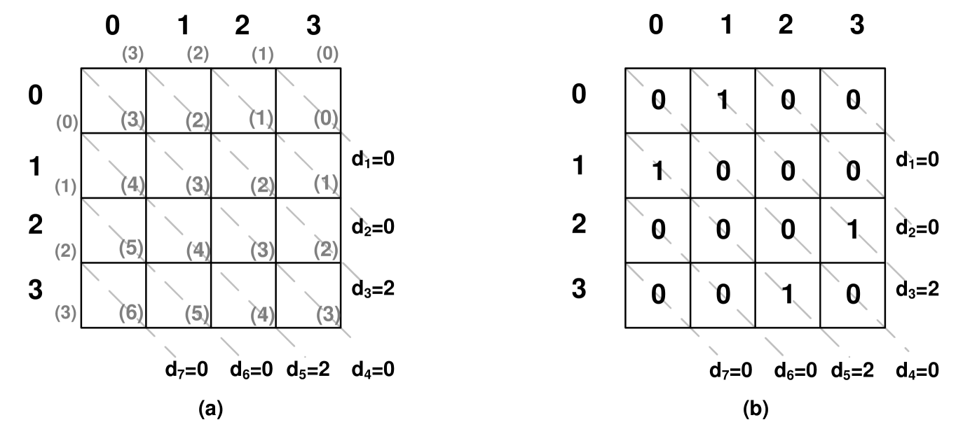
Note that each element on a diagonal is labelled with the same value. Therefore, each diagonal labelled with value represents the gap of size in the manipulation problem. Hence, the sum of the diagonal labelled with encodes the number of occurrences of gaps of size . For example, ensures that there are two gaps of size and ensures that there are two gaps of size . The remaining diagonal sums, , , are fixed to zero.
Consider a solution of PMRDS (Figure 3(b)). Cell contains the value one. Hence, we conclude that the first manipulator gives the score and the second gives the score to a candidate with the gap . Similarly, we obtain that the first manipulator gives the scores and the second gives the scores to fill gaps . As the number of ones in each diagonal is equal to the number of occurrences of the corresponding gap, the constructed two manipulator ballots make our candidate a co-winner.
Finding a coalition of two manipulators for the Borda voting rule is also connected to the problem of finding multi Skolem sequences used for the construction of Steiner triple system (?). Given a multiset of positive integers we need to decide whether there exists a partition of a set into a set of pairs , so that . There is a reduction from a manipulation problem with candidates and manipulators such that to a special case of multi Skolem sequences with similar to the reduction from a scheduling problem in (?) 111The reduction implicitly assumes that as the author confirmed in a private communication..
Conclusions
We have proved that it is NP-hard to compute how to manipulate the Borda rule with just two manipulators. This resolves one of the last open questions regarding the computational complexity of unweighted coalition manipulation for common voting rules. To evaluate whether such computational complexity is important in practice, we have proposed two new approximation methods that try to minimize the number of manipulators. These methods are based on ideas from bin packing and multiprocessor scheduling. We have studied the performance of these methods both theoretically and empirically. Our best method finds an optimal manipulation in almost all of the elections generated.
Acknowledgements
Jessica Davies is supported by the National Research Council of Canada. George Katsirelos is supported by the ANR UNLOC project ANR 08-BLAN-0289-01. Nina Narodytska and Toby Walsh are supported by the Australian Department of Broadband, Communications and the Digital Economy, the ARC, and the Asian Office of Aerospace Research and Development (AOARD-104123).
Appendix: Constructing votes with target sum
Our NP-hardness proof requires a technical lemma that we can construct votes with a given target sum.
Lemma 1
Given integers to there exist votes over candidates and a constant such that the final score of candidate is for and for candidate is where .
Proof: Our proof is inspired by Theorem 5.1 (?). We show how to increase the score of a candidate by more than the other candidates except for the last candidate whose score increases by less. For instance, suppose we wish to increase the score of candidate by more than candidates to and by more than candidate . Consider the following pair of votes:
The score of candidate increases by , of candidates to by , and of candidate by . By repeated construction of such votes, we can achieve the desired result.
References
- [Bartholdi & Orlin 1991] Bartholdi, J., and Orlin, J. 1991. Single transferable vote resists strategic voting. Social Choice and Welfare 8(4):341–354.
- [Bartholdi, Tovey, & Trick 1989] Bartholdi, J.; Tovey, C.; and Trick, M. 1989. The computational difficulty of manipulating an election. Social Choice and Welfare 6(3):227–241.
- [Brunetti, Lungo, Del, Gritzmann & Vries 2008] Brunetti, S.; Lungo, A.;A. Del; Gritzmann, P. and de Vries, S. 2008. On the reconstruction of binary and permutation matrices under (binary) tomographic constraints. Theor. Comput. Sci. 406(1–2):63–71.
- [Conitzer, Sandholm, & Lang 2007] Conitzer, V.; Sandholm, T.; and Lang, J. 2007. When are elections with few candidates hard to manipulate. JACM 54.
- [Davies et al. 2010] Davies, J.; Katsirelos, G.; Narodytska, N.; and Walsh, T. 2010. An empirical study of Borda manipulation. In COMSOC-10.
- [Hall 1935] Hall, P. 1935. On representatives of subsets. Journal of the London Mathematical Society 26–30.
- [Krause, Shen, & Schwetman 1975] Krause, K. L.; Shen, V. Y.; and Schwetman, H. D. 1975. Analysis of several task-scheduling algorithms for a model of multiprogramming computer systems. JACM 22(4):522–550.
- [Nordh 2010] Nordh, G. 2010. A note on the hardness of Skolem-type sequences. Discrete Appl. Math. 158(8):63–71.
- [Walsh 2010] Walsh, T. 2010. An empirical study of the manipulability of single transferable voting. In Proc. of the 19th European Conf. on Artificial Intelligence (ECAI-2010). IOS Press.
- [Xia et al. 2009] Xia, L.; Zuckerman, M.; Procaccia, A.; Conitzer, V.; and Rosenschein, J. 2009. Complexity of unweighted coalitional manipulation under some common voting rules. In Proc. of 21st IJCAI, 348–353.
- [Xia, Conitzer, & Procaccia 2010] Xia, L.; Conitzer, V.; and Procaccia, A. 2010. A scheduling approach to coalitional manipulation. In Parkes, D.; Dellarocas, C.; and Tennenholtz, M., eds., Proc. 11th ACM Conference on Electronic Commerce (EC-2010), 275–284.
- [Yu, Hoogeveen, & Lenstra 2004] Yu, W.; Hoogeveen, H.; and Lenstra J.K. 2004. Minimizing Makespan in a Two-Machine Flow Shop with Delays and Unit-Time Operations is NP-Hard. J. Scheduling 7(5): 333-348.
- [Zuckerman, Procaccia, & Rosenschein 2008] Zuckerman, M.; Procaccia, A.; and Rosenschein, J. 2009. Algorithms for the coalitional manipulation problem. Artificial Intelligence. 173(2):392-412.