Compositional Learning-based Planning for Vision POMDPs
Abstract
The Partially Observable Markov Decision Process (POMDP) is a powerful framework for capturing decision-making problems that involve state and transition uncertainty. However, most current POMDP planners cannot effectively handle high-dimensional image observations prevalent in real world applications, and often require lengthy online training that requires interaction with the environment. In this work, we propose Visual Tree Search (VTS), a compositional learning and planning procedure that combines generative models learned offline with online model-based POMDP planning. The deep generative observation models evaluate the likelihood of and predict future image observations in a Monte Carlo tree search planner. We show that VTS is robust to different types of image noises that were not present during training and can adapt to different reward structures without the need to re-train. This new approach significantly and stably outperforms several baseline state-of-the-art vision POMDP algorithms while using a fraction of the training time.
keywords:
Partially Observable Markov Decision Process, Monte Carlo Tree Search, Compositional Learning, Generative Models1 Introduction
Many sequential decision making problems, such as autonomous driving (Bai et al., 2015; Sunberg et al., 2017), cancer screening (Ayer et al., 2012), spoken dialog systems (Young et al., 2013), and aircraft collision avoidance (Holland et al., 2013), involve uncertainty in both sensing and planning. Planning under partial observability is challenging, as the agent must address both localization and uncertainty-aware planning through active information gathering in the environment. By capturing the observation uncertainty through a belief distribution over possible states, the agent will be able to fully close the observation-plan-action loop. While there are many methods that can either handle visual localization (Jonschkowski et al., 2018; Karkus et al., 2020, 2021) or planning under uncertainty (Van Den Berg et al., 2012; Todorov and Li, 2005), a naïve combination of these methods, for instance by assuming the certainty equivalence principle or simplifying the observation space, may not yield meaningful closed-loop control policies that enable active information gathering under more general environmental assumptions.
The partially observable Markov decision process (POMDP) formalism is a powerful framework that can capture and systematically solve these sequential decision making under uncertainty problems. However, finding an optimal POMDP policy is computationally demanding, and often intractable, due to the uncertainty introduced by imperfect observations (Papadimitriou and Tsitsiklis, 1987). One popular approach to deal with this challenge is to use online algorithms that look for local approximate policies as the agent interacts with the environment rather than a global policy that maps every possible outcome to an action, such as Monte Carlo tree search (MCTS) and similar variants (Browne et al., 2012; Silver and Veness, 2010; Sunberg and Kochenderfer, 2018; Ye et al., 2017; Kurniawati and Yadav, 2016). Many of these state-of-the-art MCTS algorithms enjoy computational efficiency (Sunberg and Kochenderfer, 2018; Mern et al., 2021; Lim et al., 2021) and finite sample convergence guarantees to the optimal policy (Lim et al., 2020, 2021). Despite their flexibility and optimality, these methods rely on having access to generative models and observation density models, which limits the class of problems they can solve in practice. In many realistic scenarios with high dimensional observations like RGB images, these POMDP methods cannot be applied without knowing or learning the relevant models or simplifying the environment.
Recently, there has been an increased interest in solving vision POMDPs, i.e. POMDPS with image or video observations, using deep learning methods. Model-free vision POMDP algorithms train an end-to-end deep neural network policy to learn both a latent belief representation and a planner (Karkus et al., 2017; Mnih et al., 2013; Igl et al., 2018), which benefit from not having to specify the transition and observation models and can learn complex policies. However, they may lack interpretability, not generalize well to new unseen tasks, and not leverage much prior knowledge about the system, especially in robotics settings. In contrast, model-based vision POMDP algorithms (Wang et al., 2020; Singh et al., 2021) combine classical filtering and planning techniques with deep learning. While such algorithmic structure allows the models to focus on specific tasks, making them sample efficient and robust, these methods often rely on simplified approaches for planning in the belief space and require learning an advantage function that only partially captures uncertainty by coupling observations with rewards.
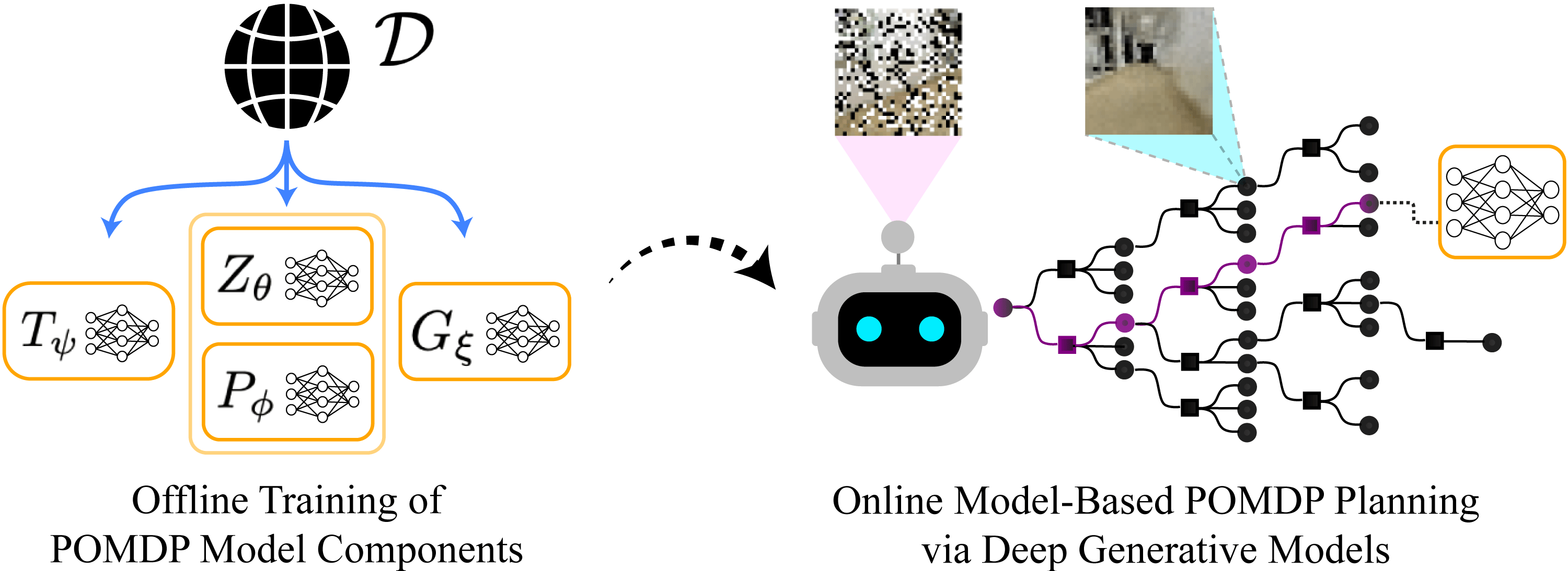
Thus, we propose Visual Tree Search (VTS), a procedure to solve vision POMDPs by combining deep generative models and online tree search planning, effectively framing the POMDP reinforcement learning problem as a compositional unsupervised learning problem. Our key insight is to utilize compositional learning approaches to bridge the offline training of individual sets of models with online model-based planning that uses learning-enabled components. Introducing the algorithmic prior knowledge of particle filtering and MCTS decreases the computational complexity required by the learning and captures state and transition uncertainty without dependence on reward structure. Our empirical analyses demonstrate that tackling uncertainty via VTS enhances performance, robustness, and interpretability of neural network components.
2 Background
POMDPs.
A POMDP is defined with a 7-tuple , with state space , action space , observation space , transition density , observation density , reward function , and discount (Kochenderfer, 2015; Bertsekas, 2005). Specifically, we say “continuous POMDPs” to denote those with continuous state, action, and observation spaces. For POMDPs, since the agent receives only noisy observations of the true state, it can infer the state by maintaining a belief at each step and updating it with the new action and observation pair via Bayesian filtering (Kaelbling et al., 1998). A policy maps a belief to an action . The agent seeks to find an optimal policy that maximizes the expected cumulative reward.
Monte Carlo Tree Search.
In Monte Carlo planning, it is not always necessary to evaluate the exact probability of all transitions and observations, and merely generating samples of next state , reward , and observation is sufficient. In particular, many Monte Carlo Tree Search (MCTS) algorithms only require that we have generative models that can generate samples with densities and , and observation density models that can evaluate the likelihood . Using these samples, MCTS can reason about the transition and observation densities by balancing exploration and exploitation to approximate the true reward distribution. This results in an approximate online policy that maximizes the expected sum of rewards at each planning step.
Deep generative models.
Many models in deep learning are used to approximate probability distributions over high dimensional spaces such as spaces of images and videos. However, sampling from these distributions requires deep generative models. While some deep generative models, such as Generative Adversarial Networks (GANs), try to sample from distributions by making the samples seem as “realistic” as possible, other models such as Variational Autoencoders (VAEs) map complex distributions to simpler ones via latent space embedding. Conditional generative models condition on another variable to sample from conditional distributions (Mirza and Osindero, 2014; Zhao et al., 2017). In our MCTS planner, we use deep generative models to sample observations conditioned on the state, and to propose state particles given the current observation. For our neural network training procedures, we make the ground truth state information available to the planner during training, but keep it unavailable during testing.
3 Related Works
Planning under uncertainty.
Planning under state and transition uncertainty requires planners to simultaneously localize and optimally plan through active information gathering. Popular control-based methods involve variants of the iterative Linear Quadratic Gaussian (Todorov and Li, 2005; Van Den Berg et al., 2012; Lee et al., 2017), which perform trajectory optimization over a simplified belief space. While such methods can handle continuous dynamics and leverage fast optimization computational tools, they cannot effectively handle image observations and high-dimensional state spaces. They also make simplifying Gaussian belief assumptions and are only locally optimal within the simplified belief space. Other sampling-based methods such as Sequential Monte Carlo (SMC) (Piché et al., 2019; Wang et al., 2020) ameliorate the above shortcomings by augmenting sampling-based planning with advantage networks, but do so at the cost of being unable to reason about future observations. Such an approximation effectively assumes that the state uncertainty vanishes at the next step, which is proven to be sometimes suboptimal (Kaelbling et al., 1998).
On the other hand, state-of-the-art tree search planners have shown success in relatively large or continuous space POMDP planning problems. Most notably, POMCPOW and PFT-DPW (Sunberg and Kochenderfer, 2018), LABECOP (Hoerger and Kurniawati, 2020), and DESPOT- (Garg et al., 2019) were shown to be effective in solving continuous observation POMDP problems. They use weighted collections of particles to efficiently represent complex beliefs. Provided the particles are weighted appropriately based on the observation likelihood, tree search using these particle beliefs will converge to a globally optimal policy (Lim et al., 2020). Furthermore, these works led to planners that can solve fully continuous or even hybrid space POMDP problems, using techniques such as continuous bandits (Lim et al., 2021) or Bayesian optimization (Mern et al., 2021). These tree search methods require access to generative models and observation density models to effectively plan, which we aim to learn with neural networks to extend the scope of the tree search methods. In this work, we integrate the PFT-DPW algorithm to handle learning-based model components.
Deep learning for vision POMDP.
Recently, there has been increased interest in solving POMDPs involving visual observations through deep learning (Guillén et al., 2005; Karkus et al., 2018; Zhang et al., 2019). Model-free vision POMDP solvers such as QMDP-net (Karkus et al., 2017) and Deep Variational Reinforcement Learning (Igl et al., 2018) maintain a latent belief vector whose update rule is learned via a neural network. They then learn corresponding value or policy networks in this latent belief state and action space. Furthermore, since these methods usually make minimal sets of assumptions, extensions of such techniques can also be seen in embodied artificial intelligence applications (Karkus et al., 2021; Ai et al., 2022)
Model-based vision POMDP works such as Differentiable Particle Filter (DPF) (Jonschkowski et al., 2018) allow conventional particle filtering techniques to be interfaced with complex visual observations. This algorithm contains multiple linked neural network components, including a particle proposer, an observation model, and a dynamics model, that are designed to be trained end-to-end. A recent work extends DPF with entropy regularization and provides convergence guarantees (Corenflos et al., 2021). Dual Sequential Monte Carlo (DualSMC) (Wang et al., 2020) extends the DPF methods further to introduce an adversarial filtering objective and integrate in the SMC planner, making it a fully closed-loop POMDP solver. In this work, we extend DPF and DualSMC to interface tree search planners.
Compositional learning.
In compositional learning, a learning task is broken down into neural network components that each specialize in different tasks. These components are then integrated to learn complex relations, allowing for less data and training resources to be used overall. Compositional learning can be achieved either through provided compositional structure in the form of an algorithmic prior (Andreas et al., 2016; Hudson and Manning, 2018), or by automatically discovering such structures (Rosenbaum et al., 2018; Alet et al., 2018; Kirsch et al., 2018; Meyerson and Miikkulainen, 2018). Specifically, algorithmic prior knowledge can be introduced by specifying neural network architectures or model components, which then allows for intelligent planning with minimal training from limited or specialized data. Furthermore, this paradigm has enjoyed success in various reinforcement learning settings, particularly multi-task problems (Devin et al., 2017; Ha and Schmidhuber, 2018; Yang et al., 2020; Mittal et al., 2020; Lim et al., 2022).
4 Visual Tree Search
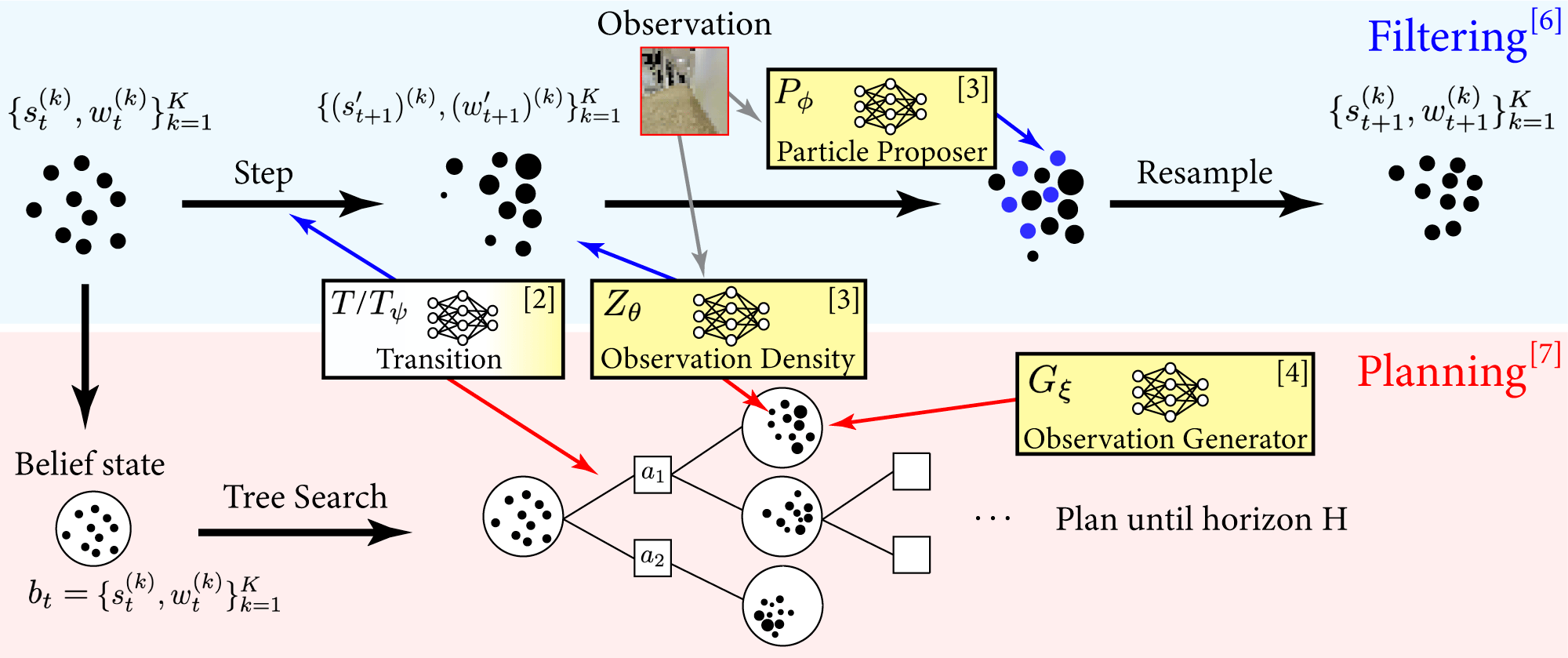
Solving a POMDP can be split into solving the filtering and the planning problems separately. In the Visual Tree Search (VTS) algorithm, we integrate the learned POMDP model components with classical filtering and planning techniques. This results in a POMDP solver that can learn model components that are more sample efficient and interpretable than end-to-end approaches. It also benefits from having a robust particle filter and planner built upon techniques with theoretical guarantees, and can adapt to different task rewards. To integrate planning techniques that use online tree search, we must have access to a conditional generative model that can generate image observations from a given state according to the likelihood density . In this section, we outline the filtering and planning algorithms and models, and the compositional training procedure.
4.1 Differentiable Particle Filtering
For particle filtering, we leverage a family of architectures called Differentiable Particle Filters (DPF) (Jonschkowski et al., 2018), which combine classical particle filtering algorithms with convolutional neural networks that can handle complex observations. We learn two neural network-based models: (1) Observation density that gives the likelihood weights , (2) Particle proposer that allows us to sample states . The Greek letters denote the parameters of these neural network models. Specifically for our work, we adapt the DPF architecture introduced in DualSMC (Wang et al., 2020), in which the observation and proposer networks are trained with an adversarial optimization objective. In principle, we can also train DPF with entropy regularization (Corenflos et al., 2021) with optimality guarantees. We assume that the transition model is known, which is not a limiting assumption for many POMDP problems (e.g. POMDPs with physical dynamics), but in principle it can be learned and modeled with a neural network as well.
The filtering procedure is described below; the belief is represented by , with as the number of particles. First, the agent takes a step with an action chosen by the planner. Then, the agent updates the predicted states with the transition model . The observation obtained from the environment is fed into the observation density , which provides the likelihood of an observation given the state. This is used to update the likelihood weights of each particle. In order to ensure robustness in the particle representation of the belief state, the particle proposer deep generative model proposes plausible state particles for a given observation, replacing some fraction of the particles. This fraction is made to decay exponentially over time.
Input: Hyperparameters for neural networks (), DPF (), MCTS (), maximum time step .
Output: Action at each step .
4.2 Tree Search Planner
Monte Carlo Tree Search.
For the online planner, we use the Particle Filter Trees-Double Progressive Widening (PFT-DPW) algorithm (Sunberg and Kochenderfer, 2018). PFT-DPW is a particle belief-based MCTS planner that is relatively easy to implement and efficiently vectorizes particle filtering. Additionally, a simplified version of PFT-DPW has optimality guarantees (Lim et al., 2020). However, any continuous POMDP tree search planner can be used instead.
For our navigation problems, we discretize the action space such that the robotic agent moves in the 8 cardinal and diagonal directions with full thrust. While this means we work with a limited action space, we can ensure that we travel with full thrust to get to the goal faster and reduce the complexity of both planning and generating observations. However, we could also work with a continuous action space in principle. Furthermore, we provide PFT-DPW with a naïve rollout policy of actuating straight towards the goal and calculating the expected reward, which PFT-DPW can use as a reference and vastly improve upon.
Observation conditional generative model.
Deep conditional generative models enable online model-based POMDP planning with images. To plan with a tree search planner, we need to be able to generate the next step states and observations, and evaluate the likelihood of the observations. With models from DPF, we can generate the next step state with transition model and calculate the likelihood weight with observation density , which are also used in the filtering procedure. Thus, we only additionally need to learn a deep generative model that generates an observation given a state : . We use a Conditional Variational Autoencoder (CVAE) (Sohn et al., 2015) to model the observation conditional generator , where the state is the conditional variable, since it had the most consistent training and performance in our experiments.
4.3 Compositional Training of Visual Tree Search
We train each neural network model with pre-collected data , containing tuples of , as shown in Lines 1-4 of Algorithm 1. We provide the and models with randomly sampled batches of state, observation, and synthetic belief particle sets . While the belief particle sets are not a part of the pre-collected data, we can easily create them by sampling states from a normal distribution centered at . The and are trained with the adversarial objective in DualSMC (Wang et al., 2020): serves as a discriminator that gives higher likelihoods to states that are more likely for a given observation, and serves as a conditional generator that proposes plausible state particles for a given observation. The model is trained with random batches of samples of state and observation pairs: . These random batches provide a good data prior for all types of states and observations an agent may encounter during planning, unlike methods such as DualSMC which only encounter data collected from the locally optimal policy.
Compared to other on-policy RL algorithms and architectures, the VTS training procedure shifts the POMDP problem from a reinforcement learning problem to a compositional learning problem, in which training each model in the POMDP is framed as an unsupervised learning problem. This drastically decreases the problem complexity, as we have explicit control over the learning objective of each model and the schedule of the training. It also allows us to better approximate the data distribution via sampling or exploration, as opposed to an evolving on-policy planner distribution that often starts off poorly and provides heavily biased data.
5 Experiments
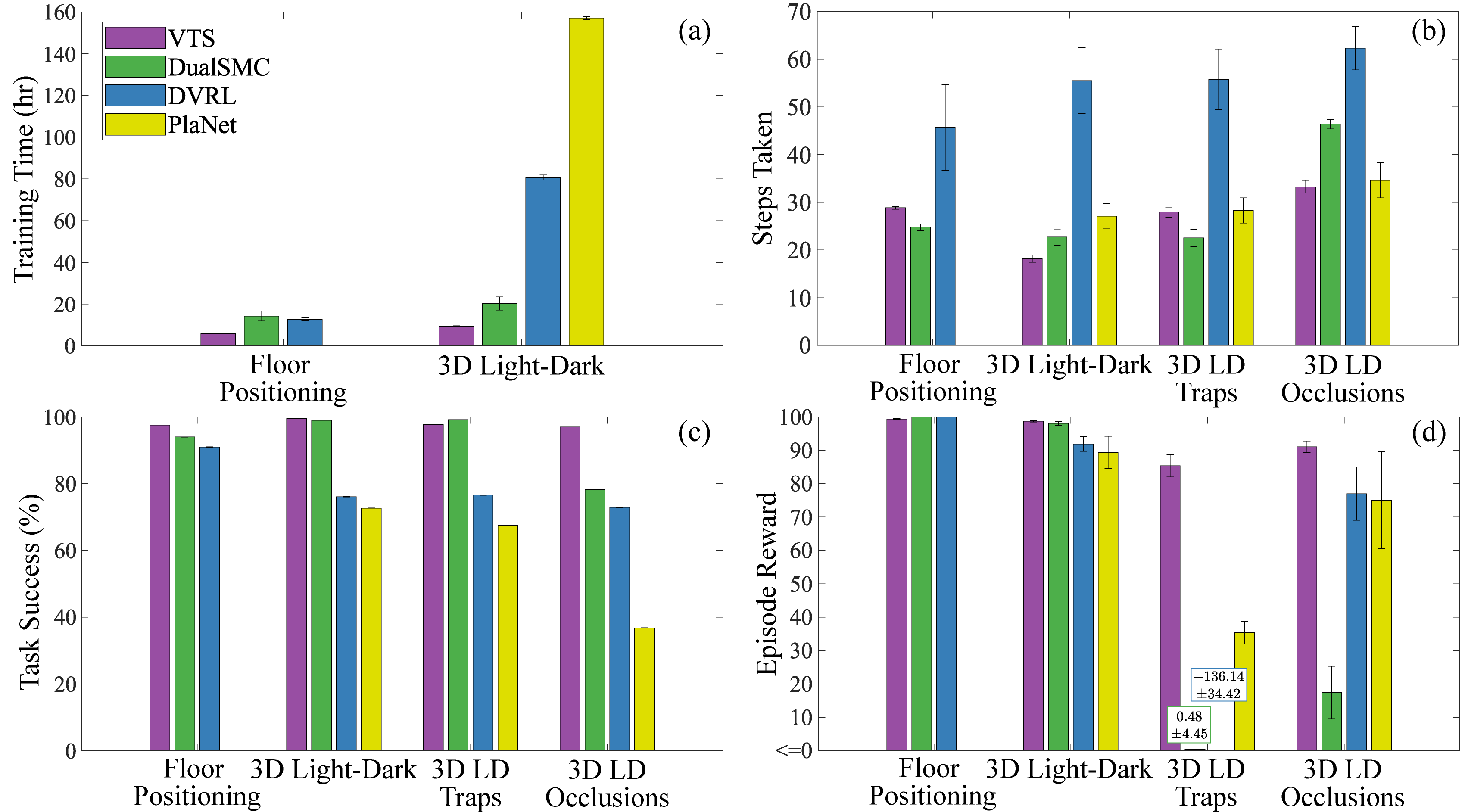
We compare VTS to other state-of-the-art vision POMDP algorithms, DualSMC (Wang et al., 2020), DVRL (Igl et al., 2018) and PlaNet (Hafner et al., 2019), on two benchmark vision POMDP problems. First, we tested our algorithm on the 2D Floor Positioning problem (Wang et al., 2020) to demonstrate that using the VTS learning and planning procedure can significantly decrease the training time to learn a solver that is agnostic to the task or reward structure of the problem. Then, we prepared our own version of the 3D Light-Dark problem in the Stanford Large-Scale 3D Indoor Spaces dataset (Armeni et al., 2017) to set up a more challenging navigation task that requires the agent to plan with realistic indoor building RGB images. We also performed ablation tests with the 3D Light-Dark experiment in which we varied the reward structure using spurious traps and the observation space using random visual occlusions. In each section, we calculate the results of the planner performances for 1000 testing episodes for Floor Positioning and 500 for 3D Light-Dark. For online planning speed, VTS takes around 0.26 seconds to plan for Floor Positioning and 0.80 seconds for 3D Light-Dark on average, while other planners require less than 0.05 seconds for both problems. The experimental summary figures are given in Fig. 3. In addition, the full tabular summary is given in Appendix A, VTS training data details in Appendix B, and the hyperparameters and computation details in Appendix C.
5.1 Floor Positioning Problem
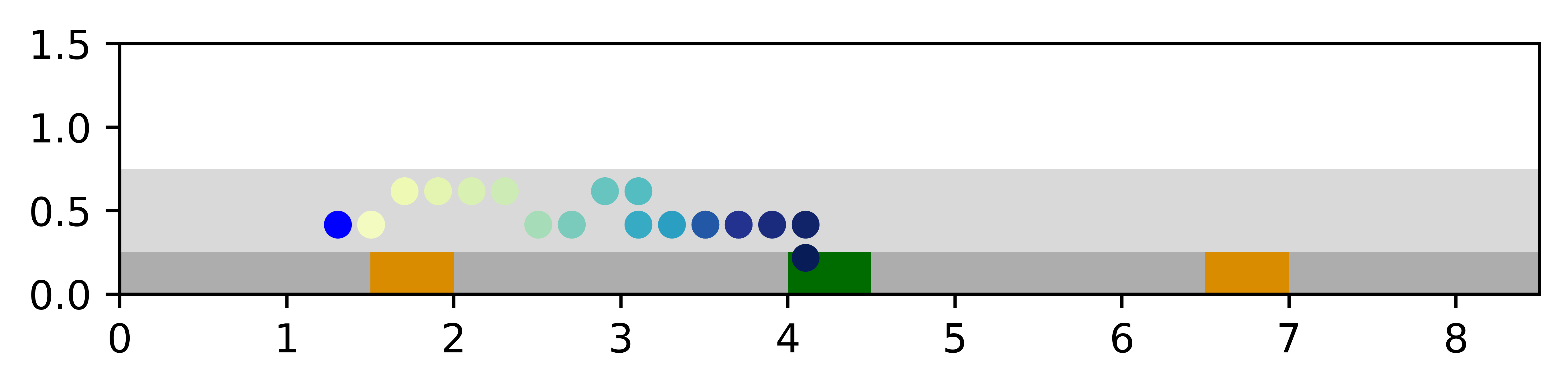
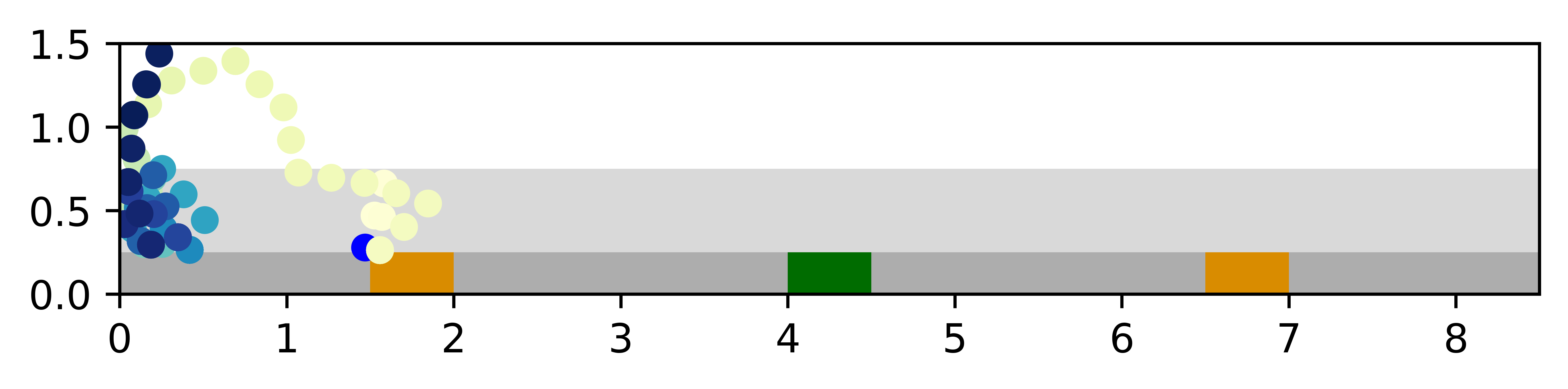
In this problem, a robotic agent is randomly placed around the center of either the top or the bottom floor, and it must infer its position by relying on a radar-like observation in all four cardinal directions, which bounces off the nearest wall. The top and bottom floors are indistinguishable within the “corridor states” of the hallways, but the robotic agent can take advantage of the “wall states” by traveling closer to the top or bottom walls of each floor, where it can receive different observations due to the different wall placements in each floor. The agent must reach the goal and avoid the trap, where the goal is the left end of the hallway in the top floor and right end in the bottom floor, and the trap is at the opposite side of the goal in each floor.
[Initial Belief]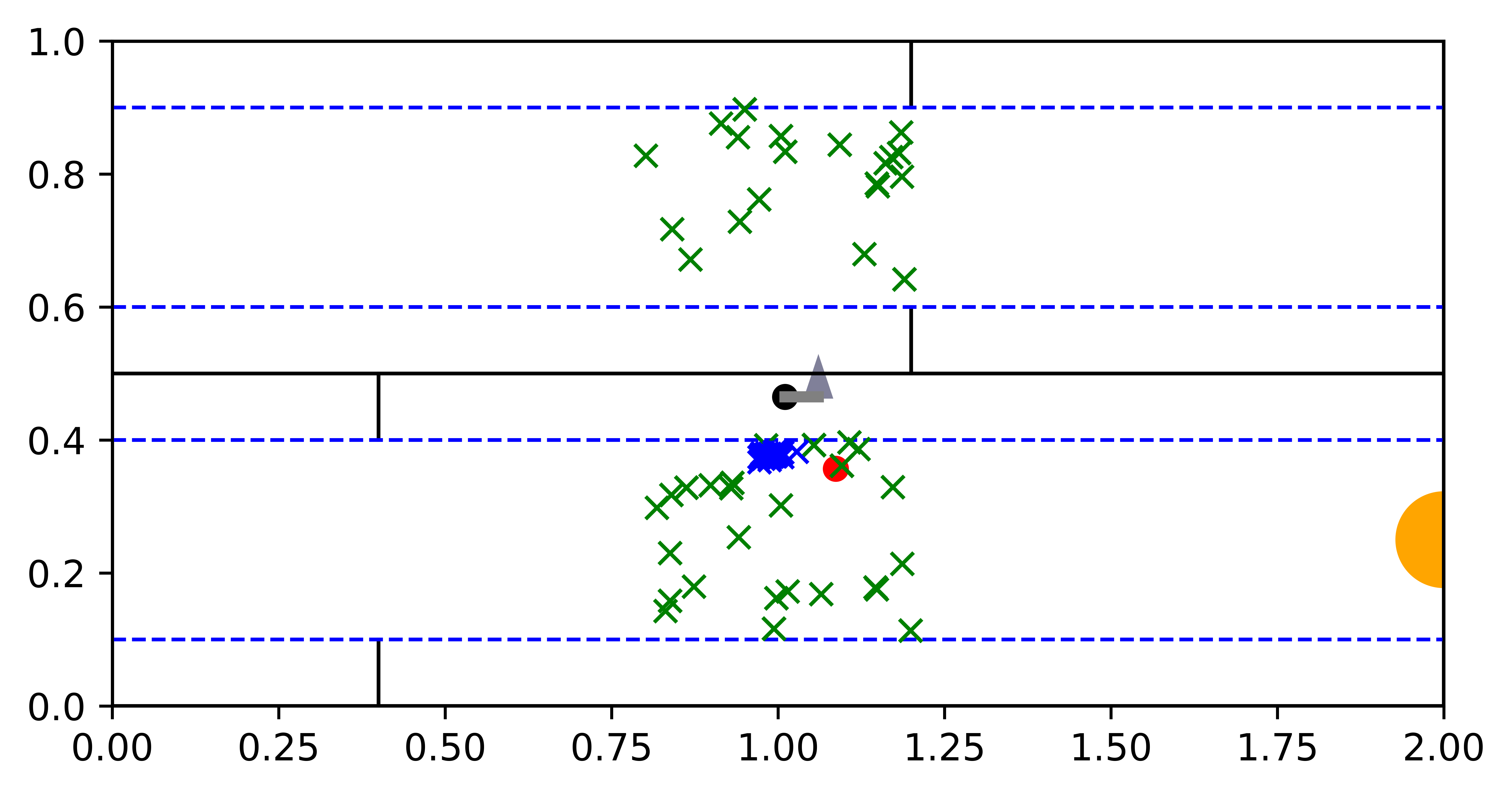 \subfigure[Localization]
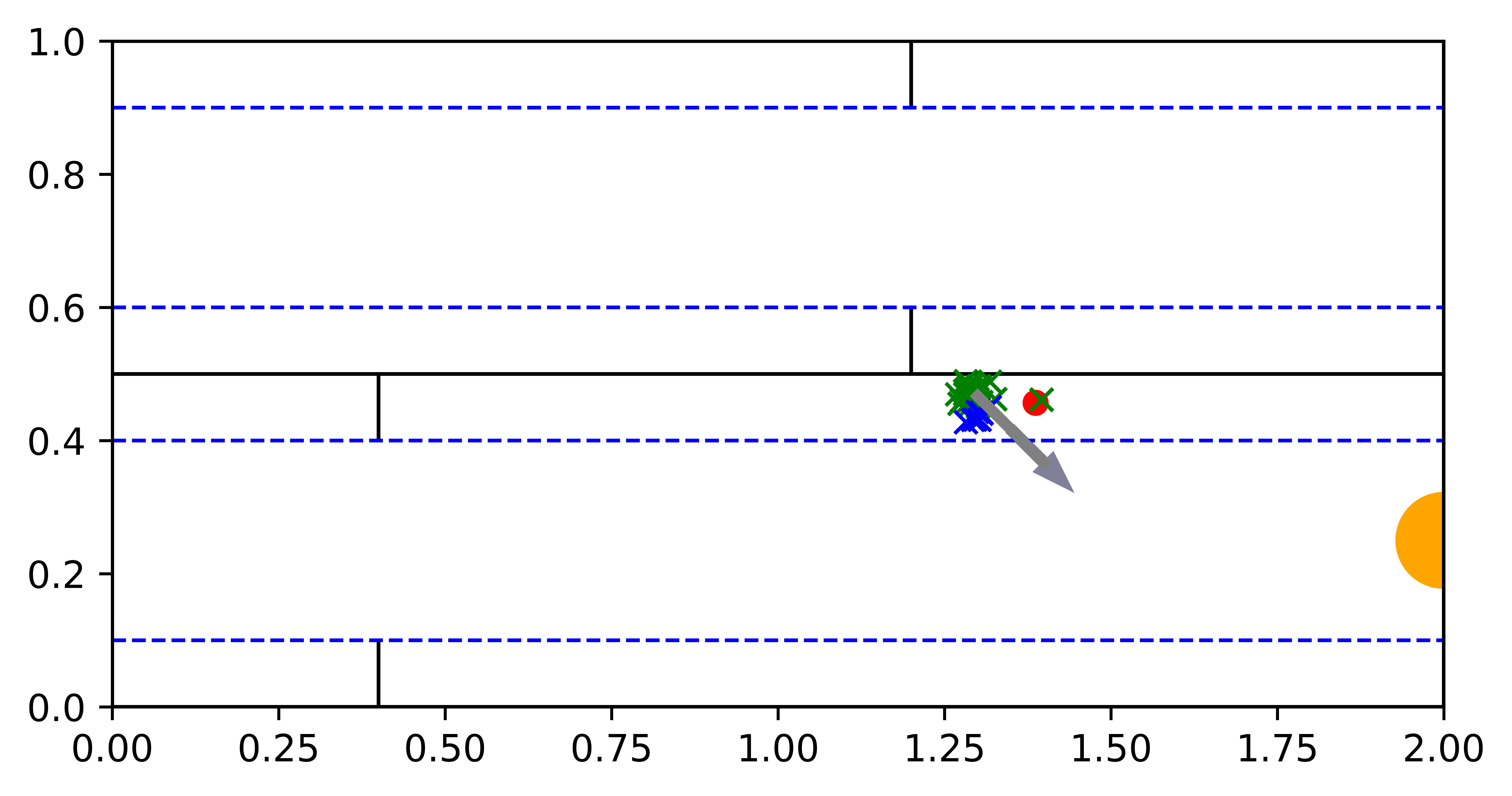 \subfigure[Reaching Goal]
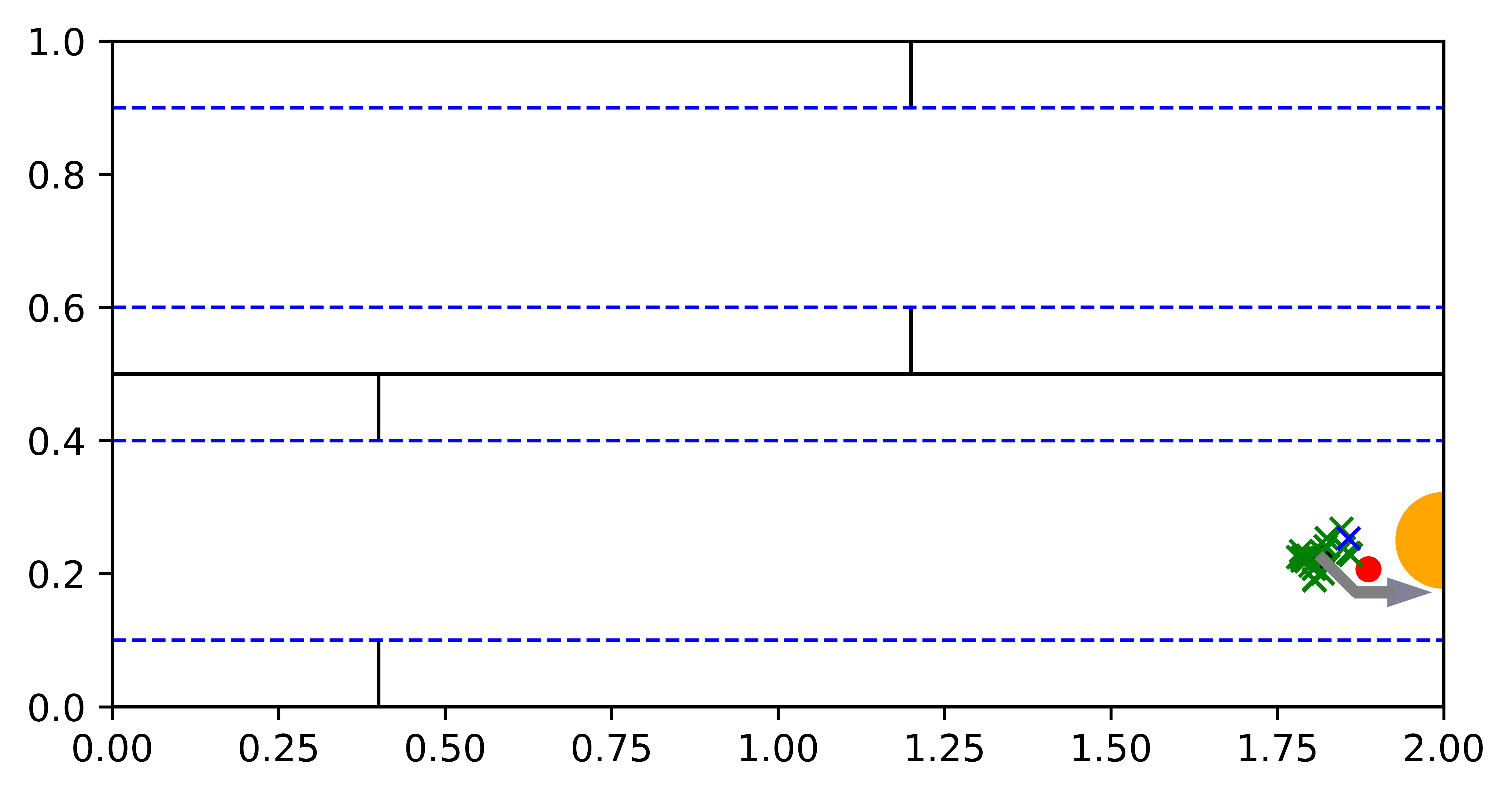
Planner comparison.
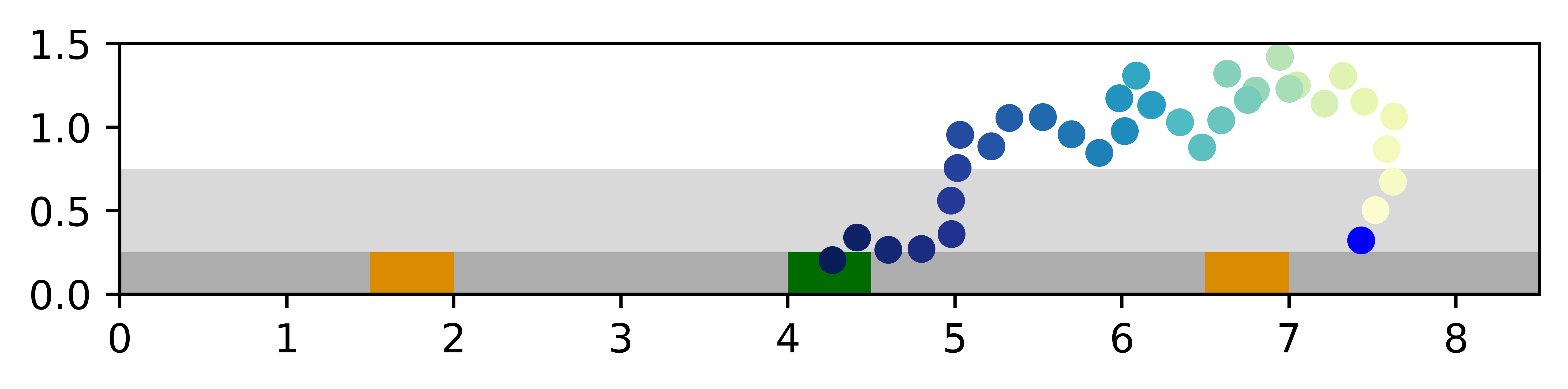
Overall, VTS is the most successful among the three planners with reasonable online planning time and steps taken, while requiring less than half the training time compared to the other planners. In Fig. 4, we show an example trajectory of the VTS agent, in which the agent quickly localizes in the wall states and then reaches the goal.
The VTS system gains significant performance optimality and efficiency by balancing offline training and online planning. Specifically, VTS training is quick since it does not rely on planner performance and only needs to be supplied with relevant state and observation batches. However, other online training algorithms require the policy to interact with the environment, and as such, much of the time is spent earlier in the training episodes when the planner can neither localize nor reach the goal. Since tree search methods learn the policy online and are more difficult to parallelize, they typically trade off the offline training time with the online learning and planning time. Despite the longer planning, VTS plans reasonably fast while maintaining the efficiency and flexibility of an online planner. We also tested DualSMC with a known model to ensure VTS is not given an advantage by knowing for model-based planning, but observed no statistically significant difference in performance.
5.2 3D Light-Dark Problem
The Light-Dark problem is a family of problems in which an agent starting in a “dark” region can localize by taking a detour into a “light” region before reaching the goal. Observations are noisier in the dark region than in the light region. The 3D Light-Dark problem extends this problem to have 3D image observations with salt-and-pepper pixel-wise noise.
The observations consist of RGB images from the agent’s perspective. Our environment is more challenging to reason with than the one in Wang et al. (2020), since the RGB images are rendered from a realistic hallway scene dataset rather than a synthetic environment. The agent receives a reward for reaching the goal and a penalty if it enters a “trap”.
Planner comparison.
In the Light-Dark problem and its variants, VTS performs the best among four planners not only by taking full advantage of the image features, but also by being able to adapt to different reward structures and distribution shifts in the noisy observations during test time. Also, DualSMC sometimes fails to have successful training seeds, and DVRL and PlaNet have lower task success rates despite all successful training seeds.
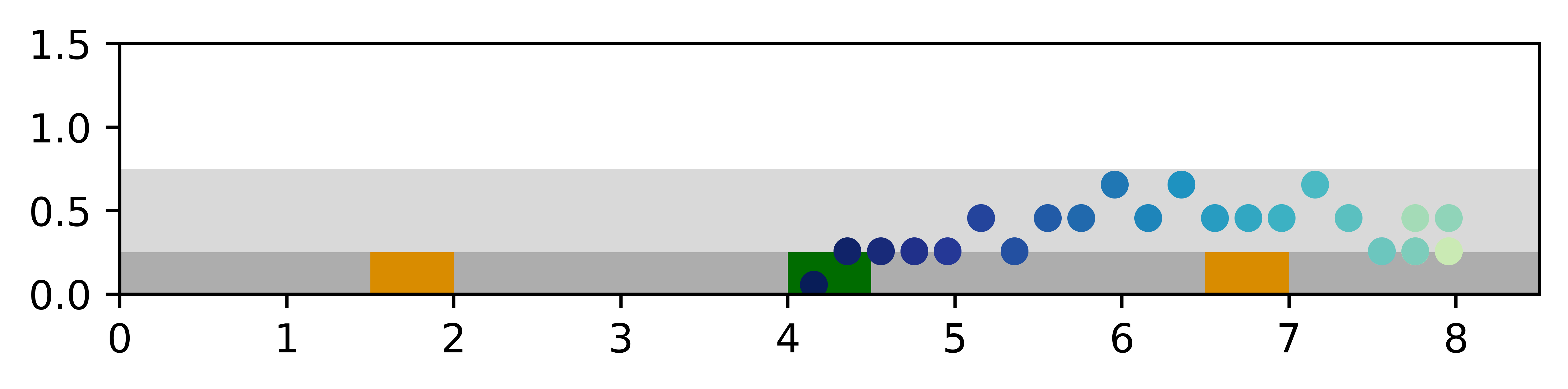
Among the successful training seeds for DualSMC, VTS and DualSMC have comparable success rates, but the VTS planner takes fewer steps to reach the goal. While this is only 4.5 steps difference on average, further inspection of the planner trajectories in Fig. 6 reveals an interesting insight. Unlike the traditional light-dark problems, the VTS results for 3D Light-Dark suggest that the planner in fact is able to localize solely with the noisy observations in the dark region. This shows that while the salt-and-pepper noise observations are hard to interpret, the corrupted RGB images actually contain sufficient information to localize given enough observations.
Test-time changes: Spurious traps.
VTS has additional advantages in its robustness and adaptability, which we showcase through experiments on modified Light-Dark environments. First, to test the adaptability of different planners on test-time reward structure difference, we perform an ablation with spurious traps that appear during test time. These regions could represent the presence of unforeseen obstacles or hazards. Over 500 testing episodes, we randomly generate the locations of two square traps over a particular strip in the environment and compare the performances of the models without additional training or modification.
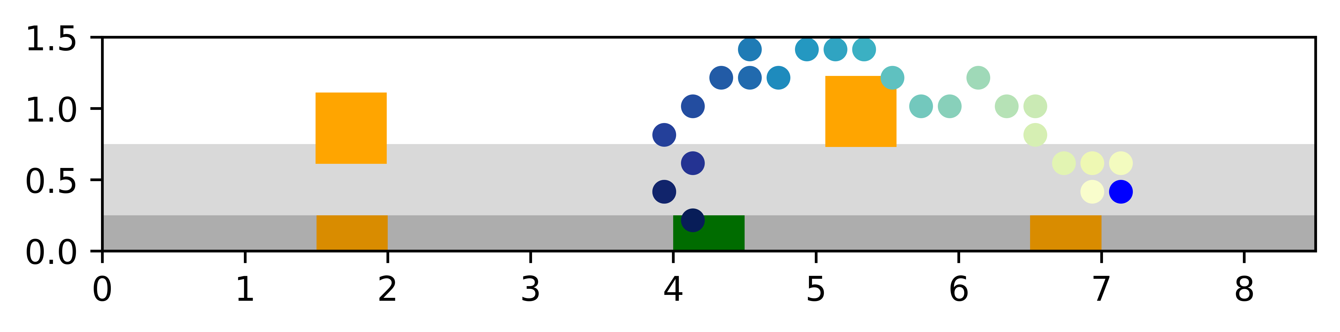
Since VTS uses an online planner, it can easily adapt to new reward structures at test time without the need to retrain an entire planner. We see in Fig. 7 that while the other planners ignore these new trap regions because they are not represented by their models, the VTS planner is able to take into account rewards seen while planning. Thus, while the success rate of all planners remains similar to the vanilla experiment, VTS achieves a much higher reward than all other planners while taking more steps as it actively tries to avoid these traps.
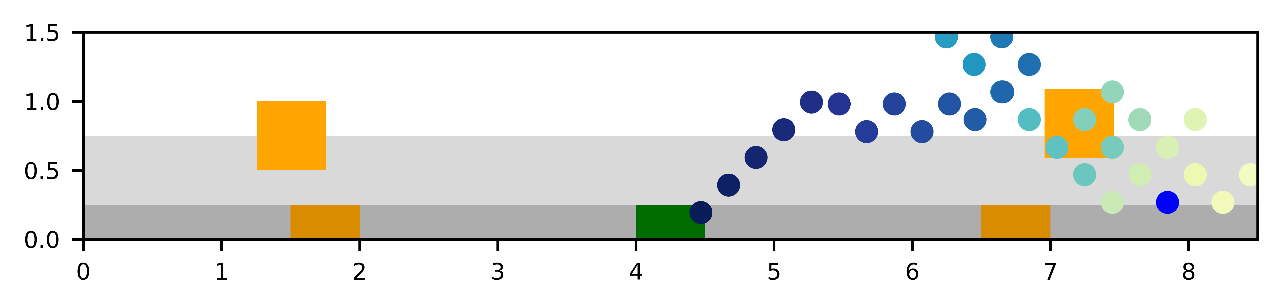
Test-time changes: Image occlusions.
Second, we compare planner performances when the form of the noise in the image observations changes during test time. During test time only, images seen in the dark region contain random blacked out squares instead of salt-and-pepper noise.
We also find that VTS is robust to distribution shifts in the image noise at test time. Fig. 8 shows VTS maintaining a good success rate and number of steps taken, while other planners are struggling to generalize to this new scenario. The additional robustness of VTS seems to be due to the and models being trained with high fidelity data samples through random batch sampling or exploration.
In contrast, other planners that use on-policy training and complex non-separable architectures suffer from such distribution shifts. This is likely due to lack of control over on-policy exploration and the inability to cover many possible scenarios with such limited interaction with the environment. Due to this difference in data variation, we conjecture that the and models in VTS learn more precise and robust features.
6 Conclusion
The development of Visual Tree Search suggests new ways to think about integrating uncertainty-aware learning and control. VTS demonstrates that a more principled integration of control and planning techniques both illuminates the interpretability of each model component and saves training time by cleanly partitioning what each network is responsible for. This benefits researchers and practitioners alike, as a more interpretable and theoretically principled planner that is also quicker to train is beneficial in many practical safety critical scenarios with limited training resources.
Our work also raises the question of what is the most natural, effective, and safety-ensured method of combining pre-existing controllers and planners, which are extensively studied both theoretically and experimentally, with learning-based components, which can model many complex functions and phenomena. VTS is one such way of accomplishing that goal, but there are other ways to achieve principled integration of learning and control.
Acknowledgments
This material is based upon work supported by a DARPA Assured Autonomy Grant No. FA8750-18-C-0101, the SRC CONIX program No. 2018-JU-2779, NSF CPS Frontiers No. CPS-1545126, the ONR Multibody Control Systems Basic Research Challenge No. N000141812214, Google-BAIR Commons, University of Colorado Boulder, the NASA University Leadership Initiative Grant No. 80NSSC20M0163, and the National Science Foundation Graduate Research Fellowship Program under Grant Nos. DGE 1752814 and DGE 2146752. Any opinions, findings, and conclusions or recommendations expressed in this material are those of the authors and do not necessarily reflect the views of any aforementioned organizations.
References
- Ai et al. (2022) Bo Ai, Wei Gao, Vinay, and David Hsu. Deep visual navigation under partial observability. In 2022 International Conference on Robotics and Automation (ICRA), pages 9439–9446, 2022.
- Alet et al. (2018) Ferran Alet, Tomas Lozano-Perez, and Leslie P. Kaelbling. Modular meta-learning. volume 87 of PMLR, pages 856–868. PMLR, 29–31 Oct 2018.
- Andreas et al. (2016) Jacob Andreas, Marcus Rohrbach, Trevor Darrell, and Dan Klein. Neural module networks. In IEEE CVPR, June 2016.
- Armeni et al. (2017) I. Armeni, A. Sax, A. R. Zamir, and S. Savarese. Joint 2D-3D-Semantic Data for Indoor Scene Understanding. ArXiv e-prints, February 2017.
- Ayer et al. (2012) Turgay Ayer, Oguzhan Alagoz, and Natasha K. Stout. A POMDP approach to personalize mammography screening decisions. Operations Research, 60(5):1019–1034, 2012.
- Bai et al. (2015) Haoyu Bai, Shaojun Cai, Nan Ye, David Hsu, and Wee Sun Lee. Intention-aware online POMDP planning for autonomous driving in a crowd. In IEEE ICRA, pages 454–460, Seattle, WA, USA, 2015. IEEE.
- Bertsekas (2005) D. Bertsekas. Dynamic Programming and Optimal Control. Massachusetts: Athena Scientific, 2005.
- Browne et al. (2012) C. B. Browne, E. Powley, D. Whitehouse, S. M. Lucas, P. I. Cowling, P. Rohlfshagen, S. Tavener, D. Perez, S. Samothrakis, and S. Colton. A survey of monte carlo tree search methods. IEEE T-CIAIG, 4(1):1–43, 2012.
- Corenflos et al. (2021) Adrien Corenflos, James Thornton, George Deligiannidis, and Arnaud Doucet. Differentiable particle filtering via entropy-regularized optimal transport. In ICML, volume 139 of PMLR, pages 2100–2111. PMLR, 18–24 Jul 2021.
- Devin et al. (2017) Coline Devin, Abhishek Gupta, Trevor Darrell, Pieter Abbeel, and Sergey Levine. Learning modular neural network policies for multi-task and multi-robot transfer. In IEEE ICRA, pages 2169–2176. IEEE, 2017.
- Garg et al. (2019) Neha P. Garg, David Hsu, and Wee Sun Lee. DESPOT-: Online POMDP planning with large state and observation spaces. In RSS, 2019.
- Guillén et al. (2005) María Elena López Guillén, Luis Miguel Bergasa, Rafael Barea, and María Soledad Escudero. A navigation system for assistant robots using visually augmented pomdps. Auton. Robots, 19(1):67–87, 2005.
- Ha and Schmidhuber (2018) David Ha and Jürgen Schmidhuber. Recurrent world models facilitate policy evolution. In NeuRIPS, pages 2451–2463. Curran Associates, Inc., 2018.
- Hafner et al. (2019) Danijar Hafner, Timothy Lillicrap, Ian Fischer, Ruben Villegas, David Ha, Honglak Lee, and James Davidson. Learning latent dynamics for planning from pixels. In International Conference on Machine Learning, pages 2555–2565, 2019.
- Hoerger and Kurniawati (2020) Marcus Hoerger and Hanna Kurniawati. An on-line POMDP solver for continuous observation spaces. ArXiv e-prints, 2020.
- Holland et al. (2013) Jessica E. Holland, Mykel J. Kochenderfer, and Wesley A. Olson. Optimizing the next generation collision avoidance system for safe, suitable, and acceptable operational performance. Air Traffic Control Quarterly, 21(3):275–297, 2013.
- Hudson and Manning (2018) Drew Arad Hudson and Christopher D. Manning. Compositional attention networks for machine reasoning. In ICLR, 2018.
- Igl et al. (2018) Maximilian Igl, Luisa Zintgraf, Tuan Anh Le, Frank Wood, and Shimon Whiteson. Deep variational reinforcement learning for POMDPs. In ICML, volume 80 of PMLR, pages 2117–2126. PMLR, 10–15 Jul 2018.
- Jonschkowski et al. (2018) Rico Jonschkowski, Divyam Rastogi, and Oliver Brock. Differentiable particle filters: End-to-end learning with algorithmic priors. In RSS, Pittsburgh, Pennsylvania, June 2018.
- Kaelbling et al. (1998) Leslie Pack Kaelbling, Michael L. Littman, and Anthony R. Cassandra. Planning and acting in partially observable stochastic domains. Artificial Intelligence, 101(1):99 – 134, 1998.
- Karkus et al. (2017) Peter Karkus, David Hsu, and Wee Sun Lee. Qmdp-net: Deep learning for planning under partial observability. In NeuRIPS, volume 30. Curran Associates, Inc., 2017.
- Karkus et al. (2018) Peter Karkus, David Hsu, and Wee Sun Lee. Integrating algorithmic planning and deep learning for partially observable navigation. ArXiv e-prints, 2018.
- Karkus et al. (2020) Peter Karkus, Anelia Angelova, Vincent Vanhoucke, and Rico Jonschkowski. Differentiable mapping networks: Learning structured map representations for sparse visual localization. In IEEE ICRA, pages 4753–4759, 2020.
- Karkus et al. (2021) Peter Karkus, Shaojun Cai, and David Hsu. Differentiable slam-net: Learning particle slam for visual navigation. In IEEE CVPR, pages 2815–2825, June 2021.
- Kirsch et al. (2018) Louis Kirsch, Julius Kunze, and David Barber. Modular networks: Learning to decompose neural computation. In NeuRIPS, volume 31. Curran Associates, Inc., 2018.
- Kochenderfer (2015) Mykel J. Kochenderfer. Decision Making Under Uncertainty: Theory and Application. Massachusetts: MIT Press, 2015.
- Kurniawati and Yadav (2016) Hanna Kurniawati and Vinay Yadav. An online POMDP solver for uncertainty planning in dynamic environment. In Robotics Research, pages 611–629. Springer, 2016.
- Lee et al. (2017) Gilwoo Lee, Siddhartha S. Srinivasa, and Matthew T. Mason. GP-ILQG: Data-driven robust optimal control for uncertain nonlinear dynamical systems. ArXiv e-prints, 2017.
- Lim et al. (2020) Michael H. Lim, Claire Tomlin, and Zachary N. Sunberg. Sparse tree search optimality guarantees in POMDPs with continuous observation spaces. In IJCAI, pages 4135–4142. International Joint Conferences on Artificial Intelligence, Inc., 7 2020.
- Lim et al. (2021) Michael H. Lim, Claire J. Tomlin, and Zachary N. Sunberg. Voronoi progressive widening: Efficient online solvers for continuous state, action, and observation POMDPs. In IEEE CDC, pages 4493–4500, 2021.
- Lim et al. (2022) Michael H. Lim, Andy Zeng, Brian Ichter, Maryam Bandari, Erwin Coumans, Claire Tomlin, Stefan Schaal, and Aleksandra Faust. Multi-task learning with sequence-conditioned transporter networks. In IEEE ICRA, pages 2489–2496, 2022.
- Mern et al. (2021) John Mern, Anil Yildiz, Zachary Sunberg, Tapan Mukerji, and Mykel J. Kochenderfer. Bayesian optimized Monte Carlo planning. In AAAI. AAAI Press, 2021.
- Meyerson and Miikkulainen (2018) Elliot Meyerson and Risto Miikkulainen. Beyond shared hierarchies: Deep multitask learning through soft layer ordering. In ICLR, 2018.
- Mirza and Osindero (2014) Mehdi Mirza and Simon Osindero. Conditional generative adversarial nets. ArXiv e-prints, 2014.
- Mittal et al. (2020) Sarthak Mittal, Alex Lamb, Anirudh Goyal, Vikram Voleti, Murray Shanahan, Guillaume Lajoie, Michael Mozer, and Yoshua Bengio. Learning to combine top-down and bottom-up signals in recurrent neural networks with attention over modules. In ICML, volume 119 of PMLR, pages 6972–6986. PMLR, 2020.
- Mnih et al. (2013) Volodymyr Mnih, Koray Kavukcuoglu, David Silver, Alex Graves, Ioannis Antonoglou, Daan Wierstra, and Martin Riedmiller. Playing atari with deep reinforcement learning. In NeurIPS Deep Learning Workshop. 2013.
- Papadimitriou and Tsitsiklis (1987) Christos H. Papadimitriou and John N. Tsitsiklis. The complexity of Markov decision processes. Mathematics of Operations Research, 12(3):441–450, 1987.
- Piché et al. (2019) Alexandre Piché, Valentin Thomas, Cyril Ibrahim, Yoshua Bengio, and Chris Pal. Probabilistic planning with sequential monte carlo methods. In ICLR, 2019.
- Rosenbaum et al. (2018) Clemens Rosenbaum, Tim Klinger, and Matthew Riemer. Routing networks: Adaptive selection of non-linear functions for multi-task learning. In ICLR, 2018.
- Silver and Veness (2010) David Silver and Joel Veness. Monte-Carlo planning in large POMDPs. In NeuRIPS, pages 2164–2172. Curran Associates, Inc., 2010.
- Singh et al. (2021) Gautam Singh, Skand Peri, Junghyun Kim, Hyunseok Kim, and Sungjin Ahn. Structured world belief for reinforcement learning in POMDP. In ICML, volume 139, pages 9744–9755. PMLR, 18–24 Jul 2021.
- Sohn et al. (2015) Kihyuk Sohn, Honglak Lee, and Xinchen Yan. Learning structured output representation using deep conditional generative models. In NeuRIPS, volume 28. Curran Associates, Inc., 2015.
- Sunberg and Kochenderfer (2018) Zachary Sunberg and Mykel J. Kochenderfer. Online algorithms for POMDPs with continuous state, action, and observation spaces. In ICAPS, Delft, Netherlands, 2018. AAAI Press.
- Sunberg et al. (2017) Zachary N. Sunberg, Christopher J. Ho, and Mykel J. Kochenderfer. The value of inferring the internal state of traffic participants for autonomous freeway driving. In ACC, pages 3004–3010, Seattle, WA, USA, 2017. IEEE.
- Todorov and Li (2005) E. Todorov and Weiwei Li. A generalized iterative lqg method for locally-optimal feedback control of constrained nonlinear stochastic systems. In ACC, volume 1, pages 300–306, 2005.
- Van Den Berg et al. (2012) Jur Van Den Berg, Sachin Patil, and Ron Alterovitz. Motion planning under uncertainty using iterative local optimization in belief space. International Journal of Robotics Research, 31(11):1263–1278, 2012.
- Wang et al. (2020) Yunbo Wang, Bo Liu, Jiajun Wu, Yuke Zhu, Simon S. Du, Li Fei-Fei, and Joshua B. Tenenbaum. Dualsmc: Tunneling differentiable filtering and planning under continuous pomdps. In IJCAI, pages 4190–4198. International Joint Conferences on Artificial Intelligence Organization, 7 2020.
- Yang et al. (2020) Ruihan Yang, Huazhe Xu, Yi Wu, and Xiaolong Wang. Multi-task reinforcement learning with soft modularization. ArXiv e-prints, 2020.
- Ye et al. (2017) Nan Ye, Adhiraj Somani, David Hsu, and Wee Sun Lee. DESPOT: Online POMDP planning with regularization. Journal of Artificial Intelligence Research, 58:231–266, 2017.
- Young et al. (2013) Steve Young, Milica Gašić, Blaise Thomson, and Jason D Williams. POMDP-based statistical spoken dialog systems: A review. IEEE, 101(5):1160–1179, 2013.
- Zhang et al. (2019) Marvin Zhang, Sharad Vikram, Laura M. Smith, Pieter Abbeel, Matthew J. Johnson, and Sergey Levine. SOLAR: deep structured representations for model-based reinforcement learning. In ICML, volume 97, pages 7444–7453, 2019.
- Zhao et al. (2017) Shengjia Zhao, Jiaming Song, and Stefano Ermon. Towards deeper understanding of variational autoencoding models. ArXiv e-prints, 2017.
Appendix
Appendix A Tabular Summary of Experimental Results
| Planner & Problem | Task | Episode | Steps | Training | Planning | Particle | |
|---|---|---|---|---|---|---|---|
| (Successful Trials) | Success (%) | Reward | Taken | Time (h) | Time (s) | Distance | |
| Floor Positioning | |||||||
| VTS | (10/10) | 97.6 | 99.36 0.12 | 28.85 | 5.88 | 0.26 | 0.07 |
| DualSMC | (10/10) | 94.0 | 100.0 | 24.78 | 14.27 | 0.04 | 0.08 |
| DVRL | (10/10) | 91.0 | 100.0 | 45.71 | 12.74 | 0.0063 e-5 | – |
| 3D Light-Dark | |||||||
| VTS | (10/10) | 99.6 | 98.71 0.22 | 18.18 0.76 | 9.42 | 0.76 0.005 | 0.48 0.07 |
| DualSMC | (6/10) | 99.0 | 98.05 0.62 | 22.71 1.70 | 20.31 | 0.06 0.003 | 0.50 0.02 |
| DVRL | (10/10) | 76.1 | 91.88 2.2 | 55.33 6.94 | 80.65 | 0.0076 e-4 | – |
| PlaNet | (4/4) | 72.7 | 89.35 4.84 | 27.1 2.67 | 157.1 | 0.061 e-4 | – |
| 3D LD + Traps | |||||||
| VTS | 97.7 | 85.34 | 27.96 | – | 0.80 | 0.42 | |
| DualSMC | 99.2 | 0.48 | 22.55 | – | 0.06 | 0.49 | |
| DVRL | 76.6 | -136.14 | 55.79 | – | 0.0076 e-4 | – | |
| PlaNet | 67.6 | 35.41 | 28.31 | – | 0.061 e-4 | – | |
| 3D LD + Occlusions | |||||||
| VTS | 97.0 | 91.05 | 33.25 | – | 0.77 | 0.82 | |
| DualSMC | 78.3 | 17.45 | 46.38 | – | 0.06 | 0.91 | |
| DVRL | 72.9 | 77.0 | 62.32 | – | 0.0075 e-4 | – | |
| PlaNet | 36.8 | 75.07 | 34.62 | – | 0.059 e-4 | – | |
For all methods, the episode length was steps. If the agent reached the goal in under steps, this was considered a success with a positive reward of and a termination of the episode. Entrance into traps incurred a negative reward of per entry. This is with the exception of DVRL, in which rewards were scaled to lie between and to ensure stability of the training. The DVRL rewards reported here are scaled by .
In addition to statistics such as the success rate, reward, and so on, we have provided values for the number of successful trials for the method. This is because certain seeds for DualSMC failed to produce any goal-reaching behavior at all during training. Since the provided statistics are only for episodes in which the goal was reached, those seeds of DualSMC were dropped entirely.
The prohibitive training time of PlaNet allowed for only trials to be run with reasonable computational resources. Training for all methods was done on NVIDIA Tesla K80 GPUs.
Note that the “planning time” reported for DVRL is actually the time to run the forward pass of the DVRL policy, since the method does not perform planning. The number has been provided to display that aspect of the algorithm.
Appendix B VTS Training Data Generation Details
The open source code for our implementations will be available at \urlhttps://github.com/michaelhlim/VisualTreeSearch.
B.1 Floor Positioning
We trained the , and models with random data batches. and were provided with random batches of samples , with being the agent’s position. The were generated from a normal distribution centered at with standard deviation 0.01. was provided with random batches of samples , where for each batch we sampled the and generated each from the corresponding . The sampling procedure for the states was biased towards the wall states, since those states were more difficult to learn from. Specifically, for and , in each batch a state would be chosen from a wall with probability and from anywhere in the environment with probability. For , in each batch a state would be chosen from a wall with probability, from a non-wall area with probability, and from anywhere in the environment with probability.
B.2 3D Light-Dark
To train the and models, we employed the following procedure. Each training batch consisted of random batches of samples , where . The agent’s location could be described by both its position and its heading , though only was unknown. In each batch, was discretely chosen from at intervals of . This is because the agent’s actions were in the form of discrete commands instantaneously changing its heading. If was in the dark region, then the were generated from a normal distribution centered at with standard deviation 0.1, and 0.01 for the light region. The difference in standard deviation was to enable the and models to cause better localization in the light region than in the dark region. The two models were trained on a schedule that gradually introduced noise in the image observations over the training epochs. In contrast, was trained simply with the random batches without the noise schedule, as if it were data collected by a randomly exploring agent. However, both sets of models could be trained either way in principle. For these conditional generative models, the concatenation of and formed the conditional variable.
B.3 On-Policy Refining
Technically, we could employ additional on-policy learning to refine the networks to focus on parts of the problem that are relevant for a given task as done in training DPF-based policies (Jonschkowski et al., 2018). However, we found that on-policy learning does not significantly improve performance in addition to regular training, since the planner often successfully and quickly reaches the goal and does not provide many new samples in areas where the models need improvement.
Appendix C Hyperparameters and Computation Details
Table 2 shows the hyperparameters used in training and filtering for VTS. Our models were trained on NVIDIA Tesla K80 GPUs. The hyperparameters for DualSMC training remained the same as the original work (Wang et al., 2020). For 3D Light-Dark, we maintained a training pool of data to draw random batches of samples from instead of generating image observations at every training step.
| Hyperparameters | Floor Positioning | 3D Light-Dark |
|---|---|---|
| Training gradient steps | 500,000 | 100,000 |
| Training sample pool size | - | 16,000 |
| Learning rate | 0.001 | 0.0003 |
| Batch size | 64 | 64 |
| Filtering particles | 100 | 100 |
| Percent of particles proposed | 0.3 | 0.3 |
| Resampling frequency | 3 | 3 |
Unlike DualSMC, VTS does not use an LSTM as one of the intermediate layers in because is trained offline from randomly collected data. We observed that this would result in particle de-localization, as the observation density could not propagate forward the localized information. In essence, the VTS solver would be quick to localize, but sometimes would need to take a detour in order to re-localize. Particle de-localization has been observed before in the literature and there are many potential methods to remedy this problem. We found an exponential decay of the number of particles proposed, as suggested by Wang et al. (2020), to provide the best results and solve the issue. That is, for episode step number and nominal particle proposal amount , the number of particles proposed is . We set the decay rate to .
Table 3 shows the hyperparameters used for PFT-DPW planner. While hyperparameters for tree search planners are often chosen with hyperparameter sweeps and/or optimization, such meta-optimization in our algorithm would mean having to run our algorithm on a GPU numerous times, which was practically very inefficient. Thus, the hyperparameters were manually chosen via a combination of inspection and prior experience. For both Floor Positioning and 3D Light-Dark, we found the rollout strategy that yielded the best results to be one in which we assume that the uncertainty in the current belief collapses in the next step. Essentially, we select a random particle from the belief and calculate its straight-line direction and distance to the goal. We use this distance to estimate the discounted reward associated with that particle. We add that with the weighted sum of rewards obtained when all other particles move in that same direction and distance.
Table 4 shows some parameters for the Floor Positioning and 3D Light-Dark environments. The environment parameters for Floor Positioning were left unchanged from Wang et al. (2020).
Across all baseline planning methods, the dimension of the action varied according to the problem in accordance with Wang et al. (2020); for the Floor Positioning problem, the action dimension was , representing a change in the 2D state. For the 3D Light-Dark problem, the action dimension was , representing a change in the agent’s orientation. DVRL, however, was found to produce the best performance when the action was 2D for both problems.
| Floor Positioning | |||||||||
| 100 | 10.0 | 3.0 | 4.0 | 100 | 10 | 0.99 | |||
| 3D Light-Dark | |||||||||
| 100 | 10.0 | 3.0 | 4.0 | 100 | 10 | 0.99 |
| Hyperparameters | Floor Positioning | 3D Light-Dark |
|---|---|---|
| Observation size | 4 | 32 32 3 |
| Agent velocity | 0.05 | 0.2 |
| Noise amount (image) | - | 40 |
| Occlusion amount (image) | - | 15 15 |
For the 3D Light-Dark problem, the and modules were trained with a gradual noise schedule that was as follows: for the first of the number of training epochs, the images in the training data had noise. For the next of the epochs, the images corresponding to states in the dark region had noise. For the next of the epochs, the images had noise. For the final of the epochs, the images had the full . (As seen in Table 4, was .) This percentage corresponds to the percent of locations on the image that were corrupted by the salt-and-pepper noise.
Finally, Table 5 shows the neural network architecture details for the models we trained on different experimental domains. We note here that although VTS and DualSMC differ in the architectures of their and models in that the networks for VTS have deeper structures than those for DualSMC, we did not see any noticeable increase in performance for DualSMC with the deeper architectures in a preliminary exploration.
| Model | Layers | # Channels |
| Floor Positioning | ||
| 5-layer MLP | ||
| Concat: state | ||
| 3-layer MLP | ||
| 3-layer MLP | ||
| Concat: | ||
| 4-layer MLP | ||
| Encoder | 5-layer MLP | , 64 |
| 1 layer to output , | 64 | |
| Decoder | 5-layer MLP | , 4 |
| 3D Light-Dark | ||
| Conv2d, filter (3, 3), stride 1 | num image channels | |
| Conv2d 4, filter (3, 3), stride 2 | 32, 64, 128, 256 | |
| Conv2d, filter (3, 3), stride 1 | 512 | |
| 3-layer MLP | 1024, 512, 256 | |
| Normalize output (*) | 256 | |
| 3-layer MLP | 256 3 | |
| Concat: state, orientation | 259 | |
| 4-layer MLP | 128 3, 1 | |
| Same as up to (*) | 256 | |
| 1-layer MLP | 256 | |
| Concat: , orientation | 513 | |
| 3-layer MLP | 128 2, 2 | |
| Encoder | Same as up to (*) | 256 |
| Concat: state, orientation | 259 | |
| 5-layer MLP | 256 4, 128 | |
| 1 layer MLP to output , | 128 | |
| Decoder | Concat , state, orientation | 131 |
| 5-layer MLP | 256 5 | |
| 3-layer MLP | 256, 512, 1024 | |
| Conv2dTranspose 3, filter (3, 3), stride 2 | 128, 64, 32 | |
| Conv2d, filter (3, 3), stride 2 | num image channels |
Appendix D Stanford 3D Light-Dark Environment Implementation Details
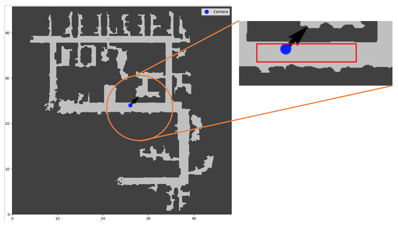
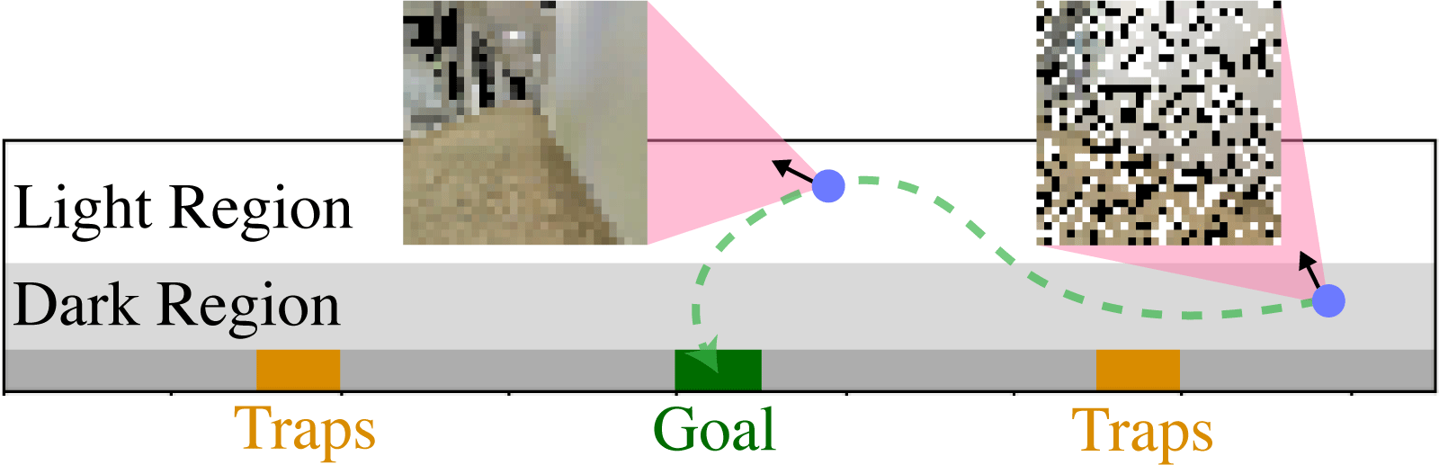
Fig. 9 shows the overview diagram of the 3D Light-Dark problem implemented using the Stanford dataset (left), and a top-down map of a floor in a building in the Stanford dataset (right).
The environment diagram depicts the “trap” regions in orange, the goal region in green, and the agent in blue. The agent’s location is given by , where are the unknown absolute position coordinates and is the known heading. The shaded part of the environment depicts the “dark” region, where the image observations received by the agent are corrupted by salt-and-pepper noise. The rest of the environment is in the “light”, where the image observations are uncorrupted. The darkest gray region is a wall region that the agent cannot enter. The agent’s initial state is randomly chosen from a strip in the dark region.
In the top-down map, the red rectangle denotes the part of the building that forms our environment (top right). We chose a subset of the Stanford dataset region in order to replicate the exact settings of the 3D Light-Dark problem in Wang et al. (2020). However, since our 3D Light-Dark implementation uses realistic images rendered with the Stanford dataset as opposed to using synthetic backgrounds generated with the DeepMind simulation platform, our problem is more realistic and challenging.
Appendix E Baseline Planner Implementation Details
We compare the performance of VTS against two baselines in addition to DualSMC: Deep Variational Reinforcement Learning for POMDPs (DVRL), and Deep Planning Network (PlaNet).
We evaluated DVRL in both the Floor Positioning and 3D Light-Dark environments and PlaNet in the 3D Light-Dark environment. This was so that we could minimally modify the model architectures provided by the two methods; while DVRL architectures supported both vector and image observations, the PlaNet architecture only supported image observations. This was also the reason for running the PlaNet 3D Light-Dark experiments with images while all other baselines and VTS used images. In this way, the baselines were advantaged in our comparisons.
E.1 DVRL
Table 6 shows the parameters modified when running DVRL, with all other parameters unchanged from the original work. For Floor Positioning, a sweep was performed over the encoder channel dimensions, presence of the BatchNorm, multiplier backprop length, and number of particles. For 3D Light-Dark, a sweep was performed over the number of environment processes, number of environment steps per gradient step, and multiplier backprop length to balance performance and computation time.
Since the DVRL implementation is designed to produce trajectories in the environment by running multiple environment processes in parallel, we performed both training and testing in this multiprocessing framework. For testing, we ran environment processes in parallel and collected the testing episodes for Floor Positioning and testing episodes for 3D Light-Dark from their combined results. Also, the DVRL policy produces actions for these parallel environments at once. Therefore, the “planning time” provided is the time for the policy to produce actions.
| Hyperparameters | Floor Positioning | 3D Light-Dark |
| Environment | ||
| Observation size | 4 | 32 32 3 |
| Agent velocity | 0.05 | 0.2 |
| Noise amount (image) | – | 40 |
| Occlusion amount (image) | – | 15 15 |
| Training | ||
| Number of training frames | 2.5e7 | 1.2e6 |
| Number of env steps per gradient step | 25 | 5 |
| Multiplier backprop length | 1 | 100 |
| Number of particles | 10 | 10 |
| Number of environment processes | 16 | 4 |
| Model | ||
| Encoder channel dimensions | ||
| BatchNorm present | Yes | Yes |
| RNN latent state size () | 256 | 256 |
| Additional latent state size () | 256 | 256 |
| Action encoding size | 64 | 128 |
E.2 PlaNet
Table 7 shows the parameters modified when running PlaNet, with all other parameters unchanged from the original work. A sweep was performed over action repeat and learning rate. The occlusion amount was increased to as compared to for the other baselines to maintain consistency with the larger image size.
Since the action repeat for the PlaNet baseline is 2, the agent only needs to perform the planning, which is done via the Cross Entropy Method (CEM), every 2 steps. This is because the action resulting from the plan is applied twice. To reflect this aspect of the algorithm in the results, we divided the obtained planning time by 2 to produce the final numbers.
| Hyperparameters | 3D Light-Dark | |
| Environment | ||
| Observation size | 64 64 3 | |
| Agent velocity | 0.2 | |
| Action repeat | 2 | |
| Noise amount (image) | 40 | |
| Occlusion amount (image) | 30 30 | |
| Training | ||
| Number of training steps | 1e6 | |
| Number of training steps per data collection phase | 100 | |
| Environment steps per data collection phase | 200 | |
| Learning rate | 1e-3 |